Optical coherence tomography measurement of retinal nerve fibre layer thickness and comparison with visual field analysis in patients with primary open angle glaucoma

Optical coherence tomography

measurement of retinal nerve fibre layer

thickness and comparison with visual

field analysis in patients with primary

open angle glaucoma

Dissertation submitted for MS (Branch III) Ophthalmology

THE TAMIL NADU DR. M.G.R MEDICAL UNIVERSITY CHENNAI

CERTIFICATE

Certified that this dissertation entitled “

Optical coherence

tomography measurement of retinal nerve fibre layer

thickness and comparison with visual field analysis in

patients with primary open angle glaucoma

” submitted for MS

(Branch III) Ophthalmology, The Tamil Nadu Dr.M.G.R.Medical

University, March 2006 is the bonafide work done by

Dr. P. M. ARAVIND

, under our supervision and guidance in the

Glaucoma Services of Aravind Eye Hospital and Post Graduate

Institute of Ophthalmology, Madurai during his residency period

from April 2003 to March 2006.

DR. S. R. KRISHNA DAS

DR. M. SRINIVASAN

Chief, Glaucoma Services

Director

Aravind

Eye

Hospital

Aravind

Eye

Hospital

ACKNOWLEDGEMENT

I acknowledge with gratitude the many people who have

contributed to the completion of this dissertation.

I thank my guide Dr. Krishna Das, Chief Medical Officer and Chief of Glaucoma services, Aravind eye hospital whose unfailing

support and unfathomable patience with me has guided me to the

undertaking of this study to successful completion.

I am forever grateful to Dr. Venkatesh Prajna, Chief, Department of Medical Education for all the help, guidance and support that he has

extended me throughout my residency programme.

I express my heartfelt thanks to Dr. G. Venkatasamy, Chairman, Dr. P. Namperumalsamy, Vice-Chairman, Dr. M. Srinivasan, Director and Dr. G. Natchiar, Director, HRD whose untiring dedication to the prevention of needless blindness in this community has inspired and will

continue to inspire innumerable young ophthalmologists like me.

I am indebted to Dr. Manju Pillai, Consultant, Glaucoma services, Dr. Nitin Deshpande and Dr. Rakhi Mehta, Fellows in Glaucoma, who reviewed my work and provided critical evaluation and support in

This dissertation could not have been completed without the team

support of the Glaucoma paramedical staff - the clinic sisters and

counsellors, and the biostatistics department.

I would fail in my duty if I didn’t thank the countless patients who

have been the learning ground for my study and my residency.

Last but not least, I thank my parents who have made me what I am

CONTENTS

PART I

1. Introduction 1

2. Review of Literature 4

3. Imaging of the Optic nerve head and Nerve Fibre layer in glaucoma 9

4. Optical Coherence Tomography 20

5. Optical Coherence Tomography in Glaucoma 29

6. Visual Field Analysis – Humphrey Field Analyser 32

PART II

7. Aims and Objectives 42

8. Materials and Methods 43

9. Proforma 47

10. Observations 50

11. Discussion and Conclusion 59

INTRODUCTION

Glaucoma is among the leading causes of irreversible blindness in the developing world and a major health problem in the developed world. 1,2 World Health Organisation statistics indicate that glaucoma accounts for blindness in 5.1 million persons, or 13.5% of global blindness. Primary open angle glaucoma is explicitly characterized as a “multifactorial optic neuropathy with a characteristic acquired loss of optic nerve fibres”, developing in the presence of open anterior chamber angles and manifesting characteristic visual field abnormalities in the absence of other known causes of the disease.3

Glaucoma is characterized by a gradual loss of retinal ganglion cells and thinning of the Retinal Nerve Fibre Layer (RNFL). Since glaucomatous damage is irreversible, prevention of this injury before it occurs is the essential strategy available to those treating this disease. The early diagnosis of glaucoma and the early detection of glaucomatous progression are twin central challenges facing ophthalmologists. 4

of the optic nerve head and stereoscopic optic nerve head photography depend on the subjective interpretation of the examiner and are thereby subject to variability in interpretation. Current diagnostic techniques such as retinal and optic nerve head analysis instruments and stereofundus photography lack sensitivity and reproducibility.6-10

Optic nerve head analyzers, developed to quantitate cupping, can measure optic nerve head rim area and provide other indices of optic nerve head structure, but can not reliably differentiate between normal and glaucomatous, and are limited in their ability to detect change over time.7-14 Improved axial resolution with reduced variability in assessing optic nerve topography is achieved with the confocal scanning laser ophthalmoscope, which produces optical sections of the retina and optic nerve head in a coronal plane. Cross-sectional imaging of the fundus with scanning laser ophthalmoscopy is limited by ocular aberrations and the pupil aperture to approximately 300 µm of axial resolution.15

measurements of RNFL thickness. Studies also have reported a decrease in OCT RNFL thickness in glaucomatous eyes compared with healthy eyes.19-23

REVIEW OF LITERATURE

A Medline literature search was performed using the key words “optical coherence tomography”, “glaucoma” and “visual fields”. The most relevant studies with respect to this dissertation were selected.

Quantification of Nerve Fibre Layer Thickness in Normal and

Glaucomatous Eyes using Optical Coherence Tomography

Schuman J, Hee MR, Puliafito CA et al Arch Ophthalmol. 1995; 113:586-596

Optical Coherence Tomography Measurement of Nerve Fibre Layer

Thickness and the Likelihood of a Visual Field Defect

Williams ZY, Schuman JS, Gamell L et al Am J Ophthalmol 2002; 134:538-546

Zinaria Y. Williams et al, in their publication tried to determine if optical coherence tomography measurements of nerve fibre layer thickness can be used to predict the presence of visual field defects associated with glaucoma. A retrospective study of OCT NFL thickness measurements in 276 eyes of 276 subjects was done; 136 eyes underwent frequency doubling technology perimetry and 140 eyes underwent Swedish Interactive threshold algorithm perimetry. They defined a parameter called NFL50, which is the NFL thickness

value at which there is a 50% likelihood of a Visual Field Defect (VFD) with either SITA or FDT perimetry. They concluded that nerve fibre thickness analysis using OCT may be clinically useful in identifying subjects who have visual field loss.

Retinal Nerve Fibre Layer Thickness Measured with Optical Coherence

Tomography is Related to Visual Function in Glaucomatous Eyes

Tarek A. El Beltagi et al studied the relationship between areas of glaucomatous retinal nerve fibre layer thinning by optical coherence tomography and areas of decreased visual field sensitivity identified by standard automated perimetry in glaucomatous eyes in their study published in 2003. They conducted a retrospective case study with 43 patients having glaucomatous optic neuropathy and imaged them with optical coherence tomography after automated perimetry. They concluded that localized retinal nerve fibre layer thinning, measured by optical coherence tomography is topographically related to decreased localized standard automated perimetry sensitivity in glaucoma patients. Also the retinal nerve fibre layer areas most frequently outside normal limits were the inferior and inferotemporal regions.

Evaluation of the glaucomatous damage on retinal nerve fibre layer

thickness measured by optical coherence tomography

Kanamori A, Nakamura M, Escano MF, et al Am J Ophthalmol. 2003;135:513-520

35 glaucoma suspect patients and 237 glaucomatous eyes of 140 glaucoma patients was done. Thickness of RNFL around the optic disc was determined with three 3.4 mm diameter circle OCT scans. Receiver operating characteristic curve area was calculated to discriminate normal eyes from early glaucomatous or glaucoma suspect eyes. A significant relationship existed between the mean deviation and RNFL thickness in all parameters excluding the 3-o’ clock area.

Retinal Nerve Fibre Layer Measurement by Optical Coherence

Tomography in glaucoma suspects with short-wavelength perimetry

abnormalities

Mok KH, Lee VW, So KF et al J Glaucoma. 2003;12:45-49

Optical Coherence Tomography Macular and Peripapillary Retinal Nerve

Fibre Layer Measurements and Automated Visual Fields.

Wollstein G, Schuman JS, Price LL, et al Am J Ophthalmol 2004;138:218-225

IMAGING OF THE OPTIC NERVE AND NERVE

FIBRE LAYER IN GLAUCOMA

The optic nerve was not visualized in living subjects routinely until Hermann von Helmholtz elaborated his ophthalmoscope in 185125. Developments in automated and static perimetry have improved the accuracy and reproducibility of documenting visual field defects but patients may lose significant neural tissue prior to the development of detectable visual field loss5. Therefore, the appearance of the optic nerve and the adjacent nerve fibre layer are the best signs of glaucoma’s presence or progression.

Although photographs supply a true picture of the ONH at a point in time, their interpretation is extremely subjective27. Technology has been introduced over the past two decades to improve the examination of the ONH, and more recently, the NFL.

OPTIC NERVE HEAD ANALYSIS

PAR IS 2000/ Topcon IMAGEnet

Optic nerve head analyzers were developed to quantitate cupping, to measure ONH rim area and to provide other indices of ONH structure. Like fundus cameras, automated systems used standard fundus cameras optics and could digitize simultaneous stereo images either directly or from 35 mm slides28_{. By using algorithms for image registration and cross-correlation to}

calculate depth values at well matched corresponding points, a three dimensional map was created of the ONH.

Humphrey Retinal Analyzer

The Humphrey Retinal Analyzer used a familiar system but input was from a red free stereoscopic video camera29.

Rodenstock Optic Nerve Head Analyzer

The Glaucoma-Scope

The Glaucoma-scope is based on the principle of raster stereography. This instrument assesses the deviation of projected lines on the ONH to reconstruct three dimensional anatomy from a monocular image. It projects 25 parallel horizontal lines onto the ONH at an angle of 90° to the ONH surface, using an infrared light source31, 32, and 33. The lines are deflected proportionately to the depth of the surface. The images are recorded on a video monitor and the deflections are translated into depth values from approximately 8750 data points. A reference surface is used and is calculated from extrapolation of the data from two vertical lines 350 µm on either side of the ONH.

Unfortunately, optic nerve head analyzers cannot reliably differentiate between normal and glaucomatous optic nerve heads and are limited in their ability to detect change over time12, 9, 13, 7, 10, 34-37. Although these systems are an attempt to automate and thus increase the objectivity of optic nerve evaluation, their accuracy and reproducibility are still limited by the optics of the systems and they still rely a great deal on human control and interpretation.

LASER SCANNING OPHTHALMOSCOPY

and ONH in a coronal plane. Scanning systems can be divided into two different categories based on the way that they detect the signal reflected back from the scanned object: confocal and non confocal.

Nonconfocal systems

In this system, a laser beam from a helium-neon, argon or infrared laser illuminates the eye. The beam is focused by the cornea onto the retina with a spot size of approximately 10 to 20 µm. The optical quality of the eye limits the minimum spot diameter. The laser beam is deflected by a rotating polygon for fast horizontal scanning and a galvanometer for slow vertical scanning to probe the fundus point by point and line by line. A partially reflective mirror separates the light backscattered from the retina and the illumination beam light. The detector receives a time-resolved image signal which is displayed on a video monitor38, 39.

A scanning imaging system is advantageous because contrast is high due to selective illumination. At any given time only the point of the retina that is to be imaged is illuminated by the laser beam.

Confocal systems

this type of imaging, only one spot on the retina is illuminated at a time through a pinhole aperture. A second small confocal aperture allows only light originating from the illuminated retinal area to pass through. The contrast is enhanced more than with nonconfocal scanning systems. Because the depth of field is dependent on the size of the detection aperture, depth of field can be varied by altering aperture diameter. When depth of field is reduced, layer by layer imaging is possible within the retina.

The Rodenstock Confocal Scanning Laser Ophthalmoscope

The Rodenstock Confocal Scanning Laser Ophthalmoscope (CSLO) obtains each focal plane image in one thirtieth of a second as a 525 horizontal line analog video signal with a field of view of 20 to 40 degrees and has a focal plane half-width thickness of 300 µm40, 38_.

Resolution with this system is dependent on laser spot size and imaging pinhole diameter rather than the optics of a fundus camera. The vertical resolution of depth is related to the spacing of the focal plane images. Although the scanning laser ophthalmoscope predominantly has served the purpose of imaging, the laser scanning tomographers provides and added feature of 3-dimensional measurements of ocular structures with good reproducibility44.

The Heidelberg Laser Tomographic Scanner

were obtained by scanning the structure point wise line by line in the given focal plane. In the case of optic disc recording, the first focal plane was defined directly above the first reflections of the retina. The last focal plane was selected in the region of the bottom of the excavation below the position of maximum reflectivity of the excavation. Within the preselected focal planes, the LTS automatically completed an optic disc scan of 32 consecutive focal plane sections from the preretinal plane to the bottom of the excavation45. Given the optical quality of the human eye, the depth resolution was 300 µm. Automatic compilation of an optic disc scan of 32 consecutive focal plane sections is done in about 4 seconds.

horizontal line. Therefore the reference plane may change over time and give inaccurate data, especially in those with glaucoma who have changing topography46. Parameters that are independent of the reference plane include cup shape, cup volume below the surface, mean cup depth, maximum cup depth, and disc area.

ONH analyzers developed to quantitate cupping can measure rim area and provide indices of structure, but cannot as yet differentiate between normal and glaucomatous nerve heads and can only make limited efforts to detect changes over time.

NERVE FIBRE LAYER ANALYSIS

The nerve fibre analyzer

The NFL has birefringent properties: back and forth travel of light through it causes a change of polarization known as retardance. Polarized light propagating through the retina is assumed to be rotated by the NFL in proportion to its thickness; therefore, measurements of the polarization state of reflected light provide information on NFL thickness. NFL thickness can be evaluated by measuring the retardance using Fourier ellipsometry50.

Scanning laser ophthalmoscope

The high visibility of the NFL resulting from the high contrast imaging inherent in the confocal laser scanning configuration can be further enhanced using digital image enhancement techniques51, 52. The confocal microscope can image NFL striations with high contrast and high lateral resolution and is not as dependent on pupil dilation or clear media as traditional photographic techniques53. The NFL striations are enhanced in this approach using digital filtering and polarization differential contrast imaging, in which changes in NFL appearance due to NFL birefringence are evaluated using two images obtained simultaneously with orthogonal polarization54.

Scanning laser polarimetry

analyzed in digital form and after adjacent scans are achieved, displayed in the form of a 256 x 256 pixel representing individual retinal positions covering 15°. The value of each pixel represents the amount of retardation – qualitatively yellow and white for high retardances while those that are dark blue represent low retardation. The time to acquire these 65,536 data locations is approximately 0.7 seconds. Measurements are obtained from a circular band of 1.5 to 2.5 disc diameters concentric to the disc. During the time of measurement, a compensation device neutralizes the corneal birefringence (but not the lenticular birefringence) to maximize polarization measurements of the retina56.

RETINAL THICKNESS MAPPING

Retinal thickness mapping with the Retinal Thickness Analyzer (RTA) is based on the principle of slit-lamp biomicroscopy in which a green 540 nm HeNe laser is projected on the fundus at an angle and its intersection with the retina is imaged. The distance between the intersection with the vitreo-retinal interface and that with the retina-retinal pigment epithelial interface is directly proportional to the retinal thickness. In about 400 ms, a 2 x 2 mm area of the fundus is scanned, yielding 10 optical cross sections that are digitally recorded and an algorithm detects points grossly deviating from their neighbours. Unlike OCT, which yields individual optic sections, the retinal thickness mapping is capable of rapidly covering the macular area and its location relative to the fovea. The RTA is limited by pupil size and it is difficult to image those eyes with numerous floaters or media opacities such as advanced cortical cataracts55.

CONFOCAL TOMOGRAPHIC ANGIOGRAPHY

NEW OBJECTIVE FUNCTIONAL TESTS

OPTICAL COHERENCE TOMOGRAPHY

The traditional view of the fundus provided by the ophthalmoscope is limited. Direct cross-sectional imaging of the retinal anatomy could benefit the early diagnosis and more sensitive monitoring of a variety of retinal and optic nerve head diseases, such as glaucoma. Current techniques for ocular imaging do not have sufficient depth resolution in the posterior segment of the eye to provide useful cross-sectional images of retinal structure. The resolution of ultrasound is limited by the acoustic wavelength in ocular tissue to about 150 µm58, 59. High-frequency ultrasound increases the resolution to about 20 µm but cannot be applied to the posterior segment owing to limited penetration60. The resolution of computed tomography and magnetic resonance imaging is also limited to hundreds of microns61, 62. Cross-sectional imaging of the fundus with scanning laser ophthalmoscopy63 and scanning laser tomography64 is limited by ocular aberrations and the numerical aperture available through the pupil, to about 300 µm64. The optical coherence tomography is a relatively new imaging modality that involves the use of a ‘low-coherence continuous-wave’ light source and ‘interferometry’. Cross-sectional information concerning retinal topography and internal tissue structure is obtained with 10 µm of longitudinal resolution from the time delay of reflected light using low-coherence

by a photodiode followed by signal-processing electronics and computer data acquisition. With 175 µW of power incident on the eye, the system is sensitive to weakly reflected light as small as 50 femtowatts.

lateral beam positioning on the retina. Retinal tomography is performed in a manner similar to indirect ophthalmoscopy, whereby a +60 dioptre (D) double aspheric condensing lens mounted on the slit lamp in front of the eye is used to relay an image of the retina onto the slit-lamp image plane. Computer control and data acquisition enable a selection of a wide range of scanning patterns on the fundus and provide a real-time display of the tomography in progress. An infrared-sensitive charge coupled device video camera attached to the slit lamp provides a video image of the scanning OCT probe beam on the fundus and permits the position of each tomography on the retina to be documented

(Figure 2). Alternatively, direct slit-lamp observation of the fundus and probe

beam may be performed using a visible aiming laser that is coupled into the OCT system and provides a visible spot coincident with the infrared probe beam on the retina65.

OCT EXAMINATION PROTOCAL

eye placing an image of the fundus is brought into focus. This adjustment compensates for differences in the refractive power between patients without being affected by accommodation in the examiner’s eye. The desired scanning position is then located while the examiner observes both the real-time display of the OCT in progress and the direct or video image of the OCT probe beam location on the fundus. The +60 D condensing lens provides a field of view of approximately 25º, which is sufficient for tomographs encompassing either, the macular or peripapillary region. Higher or lower-power condensing lenses may be interchanged to achieve either a wider field of view or higher magnification, respectively (Figure 3). The OCT examination may also be performed with an

undilated or poorly dilated pupil; however, the optical alignment is more sensitive to aperturing by the pupil and the field of view is reduced.

INTERPRETATION OF THE OCT

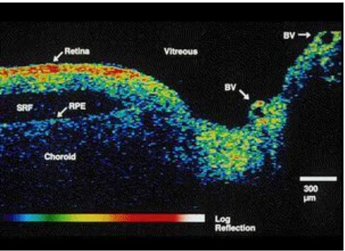
OCT differentiates between light backscattered from different depths in the retina, permitting characterization of internal retinal structure. A highly reflective red layer delineates the posterior boundary of the retina in the tomograph and probably corresponds to the retinal pigment epithelium and choriocapillaries. This posterior layer terminates at the margin of the optic disc consistent with the termination of choroidal circulation at the lamina cribrosa. Below the choriocapillaries, relatively weak reflections are observed from the deep choroid and sclera, due to attenuation of the signal passing through the retina. A dark layer indicative of minimal reflectivity appears just anterior to the choriocapillaries and pigment epithelium and probably represents the outer segments of the retinal photoreceptors. The intermediate layers of the retina anterior to these segments exhibit moderate backscattering. According to the tomograph, the RNFL increases in thickness from the macula to the optic disc as expected from normal anatomy. The reflectance from the RNFL decreases in the region of the optic disc65.

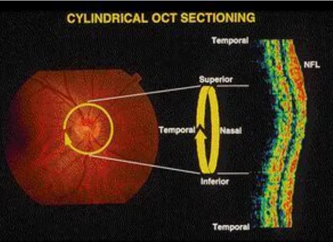
OCT FOR IMAGING THE OPTIC DISC

probe beam circularly around the disc. Each 100(horizontal) x (250 vertical) pixel image was acquired in 2.5 seconds and corresponds to a 6.75 mm radial slice through the nerve head (Figure 4). The location of each tomograph on the

retina is labelled on the fundus photograph. In the 90º tomograph (taken perpendicular to the papillomacular axis), high backscattering (red) is visible from two prominent layers that probably correspond to the RNFL and choriocapillaris (Figure 5). The tomograph shows the RNFL expanding toward

the optic disc to occupy nearly the entire retinal thickness, commensurate with the presence of the inferior and superior arcuate nerve fibre bundles. In comparison, the 0º tomograph (taken parallel to the papillomacular axis) exhibits a thinner RNFL consistent with less well-defined fibre bundles65.

OCT FOR RETINAL THICKNESS MEASUREMENT

thickness of the RNFL was also estimated by computer and was assumed to be correlated with the extent of the red, highly reflective layer at the inner margin of the retina. The Mean + S.D. for the thickness measurements were 230±15µm and 90±18µm for the retina and putative RNFL, respectively.

OCT – CIRCULAR TOMOGRAPHS IN THE PERIPAPILLARY

REGION

OCT IN GLAUCOMA

The STRAUS OCT TM 3 was used for this study and STRAUS OCT software 2.0 for analysis. The Retinal nerve fibre analysis uses three 1.73 mm radius line scans centred on the cup. The optic nerve head analysis uses six 4 mm radial line scans centred on the cup. Macular analysis uses six 4mm radial line scans centred on the fovea.

The nerve fibre layer thickness is colour coded according to the age related normal of the population. 95% of normal population falls in or below green band and 90% falls within green band. 5% of normal population falls within or below yellow band. 1% falls within red band and is considered outside normal limits (Figure 6).

The average RNFL thickness in normal and disease conditions (Schuman et al, Ophthalmol, 2003):

¾ Normal 95.9±11.4

¾ Early glaucoma 80.3 ± 18.4

¾ Advanced glaucoma 50.7 ±13.6

Mean RNFL thickness (Results of OCT from the AEH study)

Mean ±S.D. Superior 140.22± 21.17 Nasal 88.59± 21.16 Inferior 125.34± 19.71 Temporal 66.62 ±15.9

Average 104.97 ±15.14

Bilateral comparison of both eyes is possible with OCT enabling the analysis of the symmetry between the right and left eyes. Asymmetry in RNFL can be picked up as a sensitive indicator of glaucomatous loss. OCT also enables serial analysis to manage the disease and follow progression of glaucomatous damage. The software package allows analysis simultaneously of as many as four right and four left scans.

The Optic nerve head scanning takes six radial scans and gives the following data

¾ Disk area (normal 2.139mm2)

¾ Cup area (normal 0.775mm2)

¾ Rim area (normal 1.364mm2)

VISUAL FIELD ANALYSIS – HUMPHREY FIELD

ANALYSER

Two steps are involved in diagnosing glaucomatous visual field loss using automated perimetry. The first is to determine whether or not the visual field is normal. If the visual field is abnormal, the second step is to decide if the visual field abnormality is due to glaucoma or something else. When applied to perimetry, the term normal actually describes the range of test results found in the nondiseased population. The range of normal has been determined experimentally, and the results are stored in the computer memory of the automated perimeter. If all statistical parameters are within the normal range, chances are that the visual field is normal. The sensitivity of automated threshold perimetry for detecting visual field defects is very high. But the specificity of automated perimetry is often not as high as clinicians would like. When performing perimetry on patients believed to have glaucoma, it is important to distinguish the visual field that appears abnormal because of artefacts from the visual field that are truly abnormal as a result of glaucoma or some other disease such as cataract, retinal disease, or neurologic lesions66.

RELIABILITY INDICES

The fixation loss rate relates to the number of times a patient responds to a target placed in the blind spot. If the fixation loss rate exceeds 20%, it is flagged. The false-positive error rate refers to the number of times a patient responds to the audible click of the perimeter’s shutter when no target is presented. The false-negative error rate refers to the number of times a patient fails to respond to a suprathreshold (very bright) target placed in a seeing area of the visual field. The false-positive and false-negative errors are flagged if either exceeds 33%. The reliability indices are indicators of the extent to which a particular patient’s results may be reliable compared with the normal range of values stored in the computer memory67-69.

GREY SCALE

The grey scale indicates areas of high sensitivity with light shading and progressively lower sensitivities with darker shadings and so provides the reader with an overview of the pattern of visual field sensitivity. Given that this representation is based upon sampling locations within the visual field, the grey scale “fills in” areas between these tested locations by interpolation66.

GLOBAL INDICES

If a global index is outside the expected normal range, a “P” value will appear next to it. The P value represents the proportion of normal subjects in which an index of that value is found. For example, if P < 1% appears next to MD, fewer than 1% of normal subjects of that age will have an MD at that level. Any global index with a P value less than 5% has a high probability of being abnormal.

The MD is mainly an index of the size of a visual field defect. The MD is very sensitive to generalized loss of sensitivity, but purely localized defects that are large enough will also affect the MD.

The CPSD is an index of localized nonuniformity of the surface of the hill of vision. It is extremely sensitive to localized visual field defects and is not at all affected by purely generalized loss of sensitivity. By looking at the MD and the CPSD, it is possible to anticipate the nature of any visual field defect before inspecting the rest of the data.

Table 1. Interpretation of the global indices on the Humphrey visual field

analyzer

MD CPSD Interpretation

Normal Normal Visual field probably normal Abnormal Normal Generalized loss of sensitivity Normal Abnormal Small localized defect

TOTAL AND PATTERN DEVIATION

The total and pattern deviations are arrays of numbers and graphic plots in the centre and lower portions of the printout. The total deviation represents the difference between the measured threshold of each individual test location and the age-corrected normal value for that location. Visual field thresholds decline with age at the rate of between 0.5 and 1.0 decibels per decade. The pattern deviation represents the difference between an adjusted threshold of each individual test location and the age-corrected normal value for that location. The pattern deviation is derived from the total deviation by adjusting the measured thresholds upward or downward by an amount that reflects any generalized change in the threshold of the least damaged portion of the visual field.

The graphic probability plots indicate how frequently a total or pattern deviation value at a particular test location will be found in the normal population. There are four symbols ranging from P<5% to P<0.5%66.

GLAUCOMA HEMIFIELD TEST

may appear depending on the relationship of the thresholds in the superior and inferior halves of the field.

1. Within Normal Limits means that there is no significant difference between the superior and inferior halves of the fields and the overall sensitivity is within the 99.5% range of normal.

2. Outside Normal Limits appears when the threshold differences between the groups of points compared in the superior and inferior halves of the field are greater than would be expected in 99% of the normal population.

3. Borderline appears when the threshold differences are greater than would be expected in 97% of the normal population but not as great as in Outside Normal Limits.

4. General Reduction of Sensitivity appears when the overall sensitivity of the least damaged portion of the visual field is depressed below the 99.5% range of normal, but there is no significant difference between the superior and inferior halves of the field.

The specificity and sensitivity of the Glaucoma Hemifield Test for detecting nerve fibre bundle visual field defects are quite high.

CHOICE OF TEST PROGRAM

The standard test program used in glaucoma patients is the 30-2. The 24-2 eliminates the peripheral test locations of the 30-24-2 program except for the most nasal portion of the field. The 10-2 program is useful in patients with very advanced field loss who only have a small island of vision persisting near fixation. The foveal sensitivity is also a very useful piece of information and should be turned on when performing threshold perimetry in glaucoma patients. Either the full threshold or full threshold from prior data strategies should be used when performing perimetry on the Humphrey Visual Field Analyzer66_.

NATURE OF GLAUCOMATOUS VISUAL FIELD DEFECTS

NERVE FIBRE BUNDLE DEFECTS

respect the horizontal meridian, especially of the nasal portion of the field. Isolated nerve fibre bundle defects rarely cross the nasal horizontal midline and typically end there abruptly. Even in patients with more advanced visual loss due to glaucoma, a detectable difference in the measured threshold on either side of the nasal horizontal midline often occurs.

Another feature of nerve fibre bundle visual field defects is the tendency to be found in the Bjerrum area which is between 10° and 20° from fixation temporally but fans out to between 2° and 25° nasally. Scotomas in this area often assume an arcuate shape with the circumferential diameter greater than the radial diameter. Fixation itself is usually spared unless the defect is far advanced. Nerve fibre bundle defects may, however, come to within 1° of fixation.

ARTEFACTS THAT MAY RESEMBLE VISUAL FIELD DEFECTS

examination time may also be associated with depressed sensitivity and apparent visual field defects77.

AIMS AND OBJECTIVES

PURPOSE

To quantitatively assess the retinal peripapillary nerve fibre layer using optical coherence tomography and compare with standard automated perimetry in eyes with primary open angle glaucoma.

AIMS

• To quantitatively assess the retinal peripapillary nerve fibre layer in eyes with primary open glaucoma and evaluate its efficacy in diagnosing glaucoma

• To correlate the retinal nerve fibre layer thickness with a diagnostic gold standard, in this case standard automated perimetry by Humphrey’s visual field analyser

• To compare the efficacy of each of these investigations in diagnosing primary open angle glaucoma.

MATERIALS AND METHODS

A prospective study to quantitatively measure the peripapillary retinal nerve fibre layer using optical coherence tomography and compare it with standard automated perimetry using Humphrey visual field analyser in patients with primary open angle glaucoma was undertaken in the Department of Glaucoma Services, Aravind Eye Hospitals, Madurai. The study was conducted for a period of two years from1st _{July 2003 to 31}st _{July 2005 during which time}

76 eyes of 38 patients were studied and analysed.

SUBJECTS

INCLUSION CRITERIA

Best corrected visual acuity of at least 6/12 or better Age < 60 years

Patients diagnosed with Primary open angle glaucoma at the time of diagnosis or after investigation

Open angles (angle grading >2 by Shaffer’s system) Patients cooperative for visual field analysis and OCT Refractive errors

Myopia < -5D

EXCLUSION CRITERIA Age > 60 years of age

Closed angles by Gonioscopy

Media opacities – cataractous lenticular changes, vitreous haemorrhage, corneal edema/ opacity - which preclude examination of the posterior segment

Retinal pathology – advanced diabetic retinopathy, age related macular degeneration, retinitis pigmentosa, maculopathy.

All secondary glaucomas All juvenile glaucomas

All subjects had a complete ophthalmologic examination including thorough slit lamp examination, Gonioscopy, dilated direct and indirect ophthalmoscopy, intra ocular pressure measurement using Goldmann Applanation tonometry, central corneal thickness measurement and refraction.

OPTICAL COHERENCE TOMOGRAPHY

The STRAUS OCT TM 3 was used for this study and STRAUS OCT software 2.0 for analysis. The Retinal nerve fibre analysis uses three 1.73 mm radius line scans centred on the cup. The optic nerve head analysis uses six 4 mm radial line scans centred on the cup.

The OCT software measures the retinal nerve fibre layer thickness and analyses it. The nerve fibre layer thickness is colour coded according to the age related normal of the population. 95% of normal population falls in or below green band and 90% falls within green band. 5% of normal population falls within or below yellow band. 1% falls within red band and is considered outside normal limits. Retinal nerve fibre layer thickness measurements were considered outside of normal limits if they were thinner than 97.5% of normal values derived from healthy eyes in the normative database of our clinic.

STANDARD AUTOMATED PERIMETRY

Glaucomatous visual field defect was defined as a cluster of 3 or more adjacent non-edge points depressed to an extent found in less than 5 % of population (i.e., P<5%) clustered in the arcuate area,

Pattern Standard Deviation depressed to an extent found in less than 5% of the population (i.e. P<5%)

PROFORMA

Optical Coherence Tomography and Visual Fields in Primary Open angle glaucoma Study

Name: Age: Sex:

Address:

M.R.No

Diagnosis:

OCULAR EXAMINATION

Right eye Left eye

VISUAL ACUITY

Without correction With correction PUPIL

Size and shape 1. Normal 2. Altered

3. Pseudoexfoliation Reaction to light

1. Reacting briskly 2. RAPD

LENS

1. Clear 2. Cataract

3. Pseudoexfoliation

4. Subluxation/ Dislocation INTRA OCULAR PRESSURE

(By Goldmann Applanation tonometry)

Time _________________

FUNDUS

Vertical cup/ disc ratio

Notching/ Thinning of Neuroretinal rim 1. Absent

2. Superior Pole 3. Inferior Pole Disc Haemorrhages

1. Absent 2. Present Nerve Fibre Layer Defects

VISUAL FIELD DEFECTS (By Humphrey’s visual field analysis) Field defects

1. Absent

2. Superior Arcuate Scotoma 3. Inferior Arcuate Scotoma 4. Nasal Step

5. Double Arcuate Scotoma 6. Paracentral Scotoma

7. Generalized Reduction of Sensitivity Mean deviation

Pattern mean standard deviation

CENTRAL CORNEAL THICKNESS

OPTICAL COHERENCE TOMOGRAPHY

OD OS Smax

Imax

OBSERVATIONS

About The Receiver Operating Characteristic curve

Sensitivity and specificity are the basic measures of accuracy of a diagnostic test. They describe the abilities of a test to enable one to correctly diagnose disease when disease is actually present and to correctly rule out disease when it is truly absent.

However, they depend on the cut point used to define “positive” and “negative” test results. As the cut point shifts, sensitivity and specificity shift. The receiver operating characteristic (ROC) curve is a plot of the sensitivity of a test (plotted on the y-axis) versus its false-positive rate (1-specificity, plotted on the x-axis) for all possible cut points.

The accuracy of a test is measured by comparing the results of the test to the true disease status of the patient. The true disease status is determined with the reference standard procedure78.

An ROC curve demonstrates several things:

1. It shows the tradeoff between sensitivity and specificity (any increase in sensitivity will be accompanied by a decrease in specificity).

2. The closer the curve follows the left-hand border and then the top border of the ROC space, the more accurate the test.

3. The closer the curve comes to the 45-degree diagonal of the ROC space, the less accurate the test.

4. The slope of the tangent line at a cut point gives the likelihood ratio (LR) for that value of the test.

Chart 1 : Area under the receiver operator characteristic curve for optical

coherence tomography peripapillary NFL measurements for eyes with

primary open angle glaucoma

ROC Curve

1 - Specificity

1.00 .75 .50 .25 0.00 Se n s itivity 1.00 .75 .50 .25 0.00

Area Under the Curve

Test Result Variable(s): OCT

.761 .062 .000 .640 .882

Area Std. Errora

Asymptotic

Sig.b Lower Bound Upper Bound Asymptotic 95% Confidence

Interval

The test result variable(s): OCT has at least one tie between the positive actual state group and the negative actual state group. Statistics may be biased.

Under the nonparametric assumption a.

Null hypothesis: true area = 0.5 b.

Chart 2 : Area under the receiver operator characteristic curves for OCT

peripapillary NFL measurements in patients with Visual Field Defects by

Humphrey’s field analysis

ROC Curve

1 - Specificity

1.00 .75 .50 .25 0.00 Sensitivity 1.00 .75 .50 .25 0.00

Area Under the Curve

Test Result Variable(s): OCT

.686 .066 .010 .557 .814

Area Std. Errora

Asymptotic

Sig.b Lower Bound Upper Bound Asymptotic 95% Confidence

Interval

The test result variable(s): OCT has at least one tie between the positive actual state group and the negative actual state group. Statistics may be biased.

Under the nonparametric assumption a.

Null hypothesis: true area = 0.5 b.

Chart 3 : Area under the receiver operator characteristic curve for OCT

superior peripapillary NFL measurements in patients with inferior

hemifield visual defects

ROC Curve

1 - Specificity

1.00 .75 .50 .25 0.00 Se n s itivity 1.00 .75 .50 .25 0.00

Area Under the Curve

Test Result Variable(s): SMAX

.612 .078 .134 .460 .764

Area Std. Errora

Asymptotic

Sig.b Lower Bound Upper Bound Asymptotic 95% Confidence

Interval

The test result variable(s): SMAX has at least one tie between the positive actual state group and the negative actual state group. Statistics may be biased.

Under the nonparametric assumption a.

Null hypothesis: true area = 0.5 b.

Chart 4 : Area under the receiver operator characteristic curve for OCT

inferior peripapillary NFL measurements in patients with superior

hemifield visual defects

ROC Curve

1 - Specificity

1.00 .75 .50 .25 0.00 Sensitivity 1.00 .75 .50 .25 0.00

Area Under the Curve

Test Result Variable(s): IMAX

.599 .089 .236 .423 .774

Area Std. Errora

Asymptotic

Sig.b Lower Bound Upper Bound Asymptotic 95% Confidence

Interval

The test result variable(s): IMAX has at least one tie between the positive actual state group and the negative actual state group. Statistics may be biased.

Under the nonparametric assumption a.

Null hypothesis: true area = 0.5 b.

DEMOGRAPHIC STUDY POPULATION CHARACTERISTICS

Table 1 : Age Distribution

Descriptive Statistics

38 10 67 45.00 11.409

Age

N Minimum Maximum Mean Std. Deviation

Table 2 : Sex Distribution

Sex 23 60.5 15 39.5 38 100.0 Male Female Total Frequency Percent

Table 3a : Distribution of Visual field defects with Reliability indices

Descriptive Statistics

18 41 11

-1.4144 -5.1746 -13.6045

3.67160 4.34579 9.65294

18 40 11

3.1433 5.9670 8.3736

2.45162 2.95132 4.38503

eyes Mean Std. Deviation eyes Mean Std. Deviation MEAND PATTD

No VF Defect

Single hemifield

VF Defect Both hemifield VF Defect Visual Defect

Table 3 b :

ANOVA .000 .000 p-value p-value MEAND PATTD Sig.

Seventy-six eyes of 38 patients diagnosed with primary open angle glaucoma were included in the study. The mean age of the patients was 45 ±11.409 (Table 1). The gender ratio was 60.5% males and 39.5% females (Table 2). Of the 76 eyes, 18 had no demonstrable visual field defect, 41 eyes had visual field defects confined to one hemifield ( superior or inferior), and 11 eyes had field defects in both eyes (Table 3a). The ANOVA (analysis of variance) for the mean and pattern deviation in these three groups of eyes (no VF defect, Single hemifield VF defect, both hemifield VF defect) was significant (p value <0.000) (Table 3b). The average mean deviation for these eyes was -5.4736 ±6.352, and average pattern deviation was 5.5081± 3.458.

DISCUSSION AND CONCLUSION

This study was done to evaluate a relatively new diagnostic modality – the Optical coherence tomography in the diagnosis and management of Primary Open Angle Glaucoma (POAG). To achieve this we evaluated the association between functional findings as determined by perimetry, and structural findings as measured by OCT Peripapillary Nerve Fibre Layer (NFL) thickness. The assessment also included the correlation of OCT NFL measurements with ophthalmoscopically visible optic nerve head changes.

Several authors have investigated the correlation of quantitative assessment of nerve fibre layer thickness with conventional measurements of optic nerve structure and function79,80, 81. Bowd C et al80 investigated 87 eyes, to conclude that NFL thickness was significantly thinner in glaucomatous eyes than in normal eyes in each quadrant. The study also mentioned that among all quadrants inferior quadrant OCT measured NFL defects show the closest relationship to glaucoma status followed by superior quadrant NFL defects.

The current study also shows a higher AUC for the ROC of OCT in optic nerve head changes (0.761) than the AUC for the ROC of OCT in visual field defects (0.686), pointing to the fact that OCT NFL measurements are a better diagnostic test than the standard automated perimetry. This is also compounded by the fact that many cases (n=27) with normal automated perimetry showed significant peripapillary NFL thinning by OCT. This would suggest that NFL thinning measured by OCT should be considered in early glaucoma and glaucoma suspect patients who may otherwise show normal visual fields by standard automated perimetry.

Glaucoma patients could suffer a loss (approx. 40%) of retinal ganglion cell axons before an automated perimetry visual field defect is evident. Hence an advanced imaging modality like OCT is warranted in the early detection and appropriate treatment of eyes with POAG, before valuable ganglion cells and visual fields are lost permanently.

was not (0.599). This is in contrast to previous studies which showed most sensitive NFL areas to be inferior and inferotemporal areas. This might be because of smaller number of superior hemifield visual field defect cases which artificially appears to decrease its diagnostic efficacy.

The use of the Receiver Operator Characteristic curve to prove the accuracy of the diagnostic test has been done in various recent studies, showing similar area under the curve values. Williams ZY et al83 also used ROC curves to determine if OCT measurements of NFL thickness can be used to predict the presence of visual field defects associated with glaucoma. The Area under the curve for NFL in patients with visual field defects was 0.73 and was found to be significant. The current study produces similar results with an AUC of 0.76 and was significant (p<0.000).

In conclusion, the current study establishes the fact that OCT peripapillary NFL thickness measurements are indeed an accurate and sensitive diagnostic modality for detecting primary open angle glaucoma. It is effective in diagnosing patients who have very early optic nerve head changes and may suffer permanent disc changes with the progression of the disease. In comparison with automated perimetry by Humphrey’s visual field analysis, OCT corresponds well with the visual field defects defected. It is in fact more effective in predicting localized areas of NFL thinning before they may become manifest as visual field changes. Hence the use of OCT in POAG even before the appearance of visual field changes should be considered for the patient’s advantage.

Optical coherence tomography illustrates cross-sectionally the activity occurring in the NFL, a site of particular interest in glaucoma. In this study, it demonstrated thinning of the OCT peripapillary NFL in areas corresponding to visual field defects and optic nerve head changes, in agreement with several previous studies.

BIBLIOGRAPHY

1. Quigley HA: Number of people with glaucoma worldwide. Br J Ophthalmol 80:389, 1996

2. Thylefors B, Negrel AD: The global impact of glaucoma. Bull world Health Organ 72: 323, 1994

3. American Academy of Ophthalmology: Primary open-angle glaucoma: preferred practice pattern, San Francisco, 1996, The Academy.

4. Schuman SJ et al: Quantification of Nerve Fibre layer thickness in normal and glaucomatous eyes using Optical Coherence Tomography. Arch Ophthalmol 113:586-596, 1995

5. Quigley HA, Addicks EM, Green WR. Optic nerve damage in human glaucoma, III: quantitative correlation of nerve fibre loss and visual field defect in glaucoma, ischemic neuropathy, papilledema, and toxic neuropathy. Arch Opthalmol. 1982; 100:135-146

6. Lichter PR. Variability of expert observers in evaluating the optic disc. Trans Am Ophthalmol Soc. 1976; 74:532

7. Mikelberg FS, Airaksinen PJ, Douglas GR, Schulzer M, Wijsman K., The correlation between optic disk topography measured by the videoophthalmograph (Rodenstock analyzer) and clinical measurement. Am J Ophthalmol. 1985; 100:417

8. Shields MB et al, Reproducibility of topographic measurements with the optic nerve head analyzer. Am J Ophthalmol. 1987; 104:581

9. Caprioli J et al., Reproducibility of optic disc measurements with computerized analysis of stereoscopic video images. Arch Ophthalmol. 1986; 104:1035-1039

11.Balazsi GA, et al. Neuroretinal rim area in suspected glaucoma and early chronic open-angle glaucoma. Arch Ophthalmol. 1984; 102:1011-1014 12.Airaksinen PF, Drance SM, Schulzer M., Neuroretinal rim area in early

glaucoma. Am J Ophthalmol. 1985; 99:1

13.Caprioli J, et al. Videographic measurements of optic nerve topography in glaucoma. Invest ophthalmol Vis sci. 1988; 29:1294

14.Caprioli J, et al. Measurements of peripapillary nerve fibre layer contour in glaucoma. Am J Ophthalmol. 1989; 108:404

15.Bille JF, Dreher AW, Zinser G., Scanning laser tomography of the living human eye. In Masters BR, ed. Noninvasive Diagnostic Techniques in Ophthalmology. New York, NY: Springer-Verlag NY Inc; 1990; 29:1294

16.Huang D, Swanson EA, Lin CP, et al. Optical coherence tomography. Science 1991; 254:1178-1181

17.Hee MR, Izatt JA, Swanson EA, et al, Optical coherence tomography of the human retina. Arch Ophthalmol. 1995; 113:325-332

18.Chauhan DS, Marshall J. The interpretation of Optical coherence tomography images of the retina. Invest Ophthalmol Vis Sci 1999; 40:2332-2342

19.Pieroth L, Schuman JS, Hertzmark E, et al. Evaluation of focal defects of the nerve fibre layer using Optical coherence tomography: a pilot study. Arch Ophthalmol. 1995; 113:586-596

21.Hon ST, Greenfield DS, Mistlberger A, et al. Optical coherence tomography and scanning laser polarimetry in normal, ocular hypertensive, and glaucomatous eyes. Am J Ophthalmol 2000; 129:129-135

22.Bowd C, Weinreb RN, Williams JM et al., The retinal nerve fibre layer thickness in ocular hypertensive, normal and glaucomatous eyes with Optical coherence tomography. Arch Ophthalmol 2000; 118:22-26

23.Soliman MAE, Van Den Berg TJTP, Ismaeil LA, et al. Retinal nerve fibre layer analysis: relationship between Optical coherence tomography and red-free photography. Am J Ophthalmol 2002; 133:187-195

24.Quigley HA, Dunkelberger GR, Green WR. Retinal ganglion cell atrophy correlated with automated perimetry in human eyes with glaucoma. Am J Ophthalmol 1989; 107; 453-464

25.Helmholtz H. Beschreiburg eines augenspiegels zur untersuchung der netzhaut in lebnden augie. Berlin, A. Forstner, 1851

26.Lichter PR. Variability of expert observers in evaluating the optic disc. Trans Am Ophthalmol Soc 1976;74:532

27.Tielsch JM, Schwartz B. Reproducibility of photogrammetric optic disc cup measurements. Invest Ophthalmol Vis Sci 1985;26:814

28.Varma R, Spaeth GL. The PAR IS 2000. A new system for retinal digital analysis. Ophthalmic Surgery 1988;19:1183

29.Dandona L, Quigley HA, Jampel HD. Reliability of optic nerve head topographic measurements with computerized image analysis. Am J Ophthalmol 1989;108:414

31.Belyea DA, Dan JA, Lieberman MF, et al. The Glaucoma-scope: Reproducibility and accuracy of results. Invest Ophthalmol Vis Sci 1994;35:429

32.Hamzavis S, Stewart WC, Thompson TL. Inter and intraobserver variation of the optic nerve head in cadaver eyes using the Glaucoma-scope. Invest Ophthalmol Vis Sci 1993;35 (suppl): 427

33.Takamoto T, Netland PA, Schwartz B. Comparison of measurements of optic disc cup by glaucoma scope and stereophotogrammetry. Invest Ophthalmol Vis Sci 1993;35(suppl): 433

34.Balazsi GA, Drance SM, Schulzer M, et al. Neuroretinal rim area in suspected glaucoma and early chronic open angle glaucoma. Arch Ophthalmol 1984;102:1011

35.Caprioli J, Ortiz-Colberg R, Miller JM, Tressler C. Measurements of Peripapillary nerve fibre layer contour in glaucoma. Am J Ophthalmol 1989;108:404

36.Shields MB, Martone JF, Shelton AR, et al. Reproducibility of topographic measurements with the optic nerve head analyzer. Am J Ophthalmol 1987;104:581

37.Shields MB, Tiedeman JS, Miller KN, et al. Accuracy of topographic measurements with the optic nerve head analyzer. Am J Ophthalmol 1989;107:273

38.Plesch A, Klingbeil U, Rappl W, et al. Scanning ophthalmic imaging. In Nasmann JE, Burk ROW (eds). Scanning laser ophthalmoscopy and tomography. Munchen, Quintessenz, 1990, p 23-37

39.Webb RH, Hughes GW, Delori FC. Confocal scanning laser ophthalmoscope. Applied Optics, 1987;26:1492

41.Kino GS, Corle TR. Confocal scanning optical microscopy. Physics Today 1989;42:55

42.Masters BR, Kino GS. Confocal microscopy of the eye. In Masters BR (ed). Noninvasive Diagnostic Techniques in Ophthalmology. New York, Springer-Verlag, 1990, pp 152-171

43.Schuman H, Murray JM, Di Lullo C. Confocal microscopy. An overview. Bio Techniques 1989;7:154

44.Billie JF, Dreher GW, Zinser G. Scanning laser tomography of the living human eye. In Masters BR (ed); Noninvasive Diagnostic Techniques in Ophthalmology. New York, Springer-Verlag, 1990, pp 528-547

45.Dreher AW, Tso PC, Weinreib RN. Reproducibility of topographic measurements of the normal and glaucomatous optic nerve head with the laser tomographic scanner. Am J Ophthalmol, 1991;111:221

46.Mikelberg F, Wijsman K, Schulzer M. Reproducibility of topographic parameters obtained with the Heidelberg retina tomography. J Glaucoma, 1993;2:101-103

47.Quigley HA, Addicks EM, Green WR. Optic nerve damage in human glaucoma. Arch Ophthalmol 1982;100:135

48.Quigley HA, Addicks EM. Quantitative studies of retinal nerve fibre layer defects. Arch Ophthalmol 100:807-814,1982

49.Quigley HA, Miller NR, George T. Clinical evaluation of nerve fibre layer atrophy as an indicator of glaucomatous optic nerve damage. Arch Ophthalmol,1980;98:1564-1571

51.Dreher AW, Reiter K, Weinreb RN. Spatially resolved birefringence of the retinal nerve fibre layer assessed with a retinal laser ellipsometer. Applied Optics 1992;31:3730-3735

52.Weinreb RN, Dreher AW, Coleman A, et al. Histopathologic validation of Fourier-ellipsometry measurements of retinal nerve fibre layer thickness. Arch Ophthalmol 1990;108:557

53.Dreher AW, Reiter K. Retinal laser ellipsometry: A new method for measuring the retinal nerve fibre layer thickness distribution? Clinical Vision Sciences,1992;7: 481-488

54.Morsman CD, Karwatowski WSS, Wienreb RN. Reproducibility of retinal nerve fibre layer thickness measurements by scanning laser polarimetry and correlation with red free photography in normal eye. Invest Ophthalmol Vis Sci 1993;34(suppl):1507

55.Zeimer R, Shahidi M, Mori M, et al. A new method for rapid mapping of the retinal thickness at the posterior pole. Invest Ophthalmol Vis Sci 1996;37:1994-2001

56.Schuman JS, Kim Joshua, Imaging of the optic nerve head and nerve fibre layer in glaucoma. Ophthalmol Clinics of North America, 2000;13:383-406

57.Schuman JS, Noecker RJ, Imaging of the optic nerve head and nerve fibre layer in glaucoma. Ophthalmol clinics of North America, 1995; 8:259-280

58.Olsen T. The accuracy of ultrasonic determination of axial length in pseudophakic eyes. Acta Ophthalmol (Copenh) 1989; 67:141-144

60.Pavlin CJ, et al. Clinical use of ultrasound biomicroscopy. Ophthalmology. 1990; 98:287-295

61.Chang DF. Ophthalmic examination. In: General Ophthalmology. 13th ed. 1992:30-62

62.Seiler T, Bende T. Magnetic resonance imaging of the eye and orbit. Noninvasive Diagnostic Techniques in Ophthalmology. 1990:17-31 63.Webb RH, et al. Confocal scanning laser ophthalmoscope. Appl Opt.

1987;26:1492-1499

64.Bille JF et al. Scanning laser tomography of the living human eye. Noninvasive

Diagnostic Techniques in Ophthalmology. 1990:528-547

65.Hee MR et al. Optical Coherence Tomography of the Human Retina. Arch Ophthalmol. 1995; 113:325-332

66.Werner EB, Interpreting automated visual fields. Ophthalmology Clinics of North America. 1995; 8:229-258

67.Heijl A et al. Extended empirical statistical package for evaluation of single and multiple fields in glaucoma: Statpac2. Perimetry update 1991, pp 303-315

68.Heijl A: Reliability parameters in computerized perimetry. Seventh International Visual Field Symposium, 1987, pp 593-600

69.Heijl A: A package for the statistical analysis of visual fields. Seventh International Visual Field Symposium, 1987, pp 153-168

70.Flammer J. The concept of visual field indices. Graefes Arch Clin Exp Ophthalmol, 1986; 224:389-392

72.Aman P, Heijl A. Glaucoma hemifield automated visual field evaluation. Arch Ophthalmol 1992; 110: 812-819

73.Asman P, Heijl A. Evaluation of methods for automated hemifield analysis in perimetry. Arch Ophthalmol 1992; 110: 820-826

74.Anderson DR. Automated Static Perimetry. St. Louis, MO, Mosby Year Book 1992, pp 10-93

75.Radius RL. Anatomy and pathophysiology of the retina and the optic nerve. The Glaucomas. St. Louis, CV Mosby, 1989, pp 89-132.

76.Lindenmuth KA, et al. Effects of papillary constriction on automated perimetry in normal eyes. Ophthalmology, 1989; 96:1298-1301

77.Searle AET, Wild JM, Shaw DE, et al. Time-related variation in normal automated perimetry. Ophthalmology 1991; 98: 701-707

78.Obuchowski Nancy A., Receiver Operating Characteristic curves and their use in Radiology, 2003; 229: 3-8

79.Schuman JS, et al. Quantification of Nerve Fibre Layer Thickness in Normal and Glaucomatous Eyes Using Optical Coherence Tomography. Arch Ophthalmol. 1995; 113: 586-596

80.Bowd C et al. The Retinal Nerve Fibre Layer Thickness in Ocular Hypertensive, Normal and Glaucomatous Eyes with Optical Coherence Tomography. Arch Ophthalmol. 2000; 118 : 22-26

81.Kanamori A, Nakamura M, Escano MF, et al. Evaluation of the glaucomatous damage on retinal nerve fibre layer thickness measured by optical coherence tomography. Am J Ophthalmol. 2003;135:513-520 82.El Beltagi TA, Bowd C, Boden C,et al. Retinal Nerve Fibre Layer

83.Williams ZY, Schuman JS, Gamell L et al. Optical Coherence Tomography Measurement of Nerve Fibre Layer Thickness and the Likelihood of a Visual Field Defect. Am J Ophthalmol 2002; 134:538-546

84.Mok KH, Lee VW, So KF et al. Retinal Nerve Fibre Layer Measurement by Optical Coherence Tomography in glaucoma suspects with short-wavelenght perimetry abnormalities. J Glaucoma. 2003;12:45-49

Figure 2 : The CARL ZEIS STRAUSS Optical Coherence Tomography

Fig 6 : RN

FL TH

IC

KN

ESS AVERAGE ANALYSIS

Sectoral

A

n

alysis

T

a

bulated An

alysi

Fig 7: Cor

relation of ONH ch

an

ges and Visual Fields

w

ith

Optical Cohere

nce Tomography

Fundus Photogr

aph

Visual Field

Optical Coherence Tomogr

aphy

Medical

Record

No. RE LE RE LE RE LE RE LE RE LE RE LE RE LE RE LE RE LE RE LE RE LE RE LE RE LE

1 KASTHURI.N 55 2 1942545 6/36 6/36 6/6 6/6 16 16 0.60 0.70 2 3 1 2 1 2 2 3 -6.77 -9.46 8.60 12.06 160.0 149.0 179.0 123.0 93.58 81.06 2 RENGASAMY 38 1 2020775 6/6 6/6 30 30 0.90 0.85 1 1 1 1 3 2 2 2 -11.93 -11.66 8.34 8.50 119.0 125.0 97.0 111.0 72.00 79.04 3 JAMES.M 45 1 1966383 6/6 6/6 14 16 0.80 0.80 1 2 1 1 1 3 1 1 3.28 -0.12 3.53 3.64 148.0 140.0 126.0 134.0 88.91 75.62 4 DEVADASS 50 1 1006239 6/6P 6/6 6/6P 6/6 20 20 0.65 0.85 1 1 1 1 1 2 1 4 0.44 -3.14 1.53 6.07 162.0 118.0 166.0 89.0 117.00 77.00 5 SHEBA SHUTOOR 32 2 1967263 6/9 6/60 6/6 6/6 10 9 0.70 0.60 2 2 1 1 1 1 3 1 -2.59 -1.23 6.63 1.98 106.0 123.0 193.0 176.0 89.95 91.47 6 SHOBA NAIR 39 2 1151484 6/12 6/9 6/6 6/6 12 10 0.75 0.50 3 1 1 1 1 1 2 1 -2.34 0.68 7.30 1.42 127.0 169.0 114.0 164.0 81.38 95.70 7

SAKUNDALA

SELVARAJ.S 56 2 1609107 6/9 6/9 6/6 6/6 16 18 0.80 0.60 2 3 1 1 1 1 5 5 -11.13 -13.22 8.33 10.66 110.0 165.0 112.0 182.0 74.80 101.88 8 GURUSAMY.N 32 1 941288 6/6 6/6 16 12 0.75 0.50 2 1 1 1 1 1 3 3 -8.10 -7.10 8.77 7.32 83.0 175.0 156.0 153.0 79.80 101.69 9 MANI.K 53 1 1940776 6/12 6/12 6/6 6/6 13 14 0.75 0.80 3 3 1 1 2 1 2 2 -8.21 -6.36 11.80 8.90 105.0 51.0 64.0 64.0 54.72 44.04 10 AMUTHAVENI.P 35 2 1514437 5/60 5/60 6/6 6/6 20 19 0.75 0.75 3 1 1 1 1 1 4 2 -1.51 -2.32 2.36 2.72 134.0 163.0 115.0 139.0 84.71 95.78 11 KALPANA 58 2 1671211 6/60 6/36 6/9 6/6 20 18 0.70 0.40 3 1 1 1 1 1 1 1 -5.37 -3.88 2.47 1.77 123.0 104.0 171.0 151.0 85.54 80.44 12 HERIC MANI 49 1 2000737 6/6 6/6 20 20 0.80 0.80 3 3 1 1 1 1 2 1 -2.65 -1.16 4.06 1.73 107.0 124.0 148.0 149.0 74.28 81.50 13 BABU.G 38 1 1773110 2/60 2/60 6/12 6/9 25 20 0.80 0.85 1 1 1 1 1 1 4 3 -13.42 -23.57 9.90 11.98 59.0 58.0 53.0 52.0 38.91 41.58 14 MOIDEEN KOYA.CP 39 1 1935527 6/6 6/6 16 16 0.70 0.80 1 1 1 1 1 1 3 3 -8.58 -5.33 9.71 3.43 166.0 79.0 120.0 109.0 86.99 63.53 15 VARSHINI 10 2 1659821 6/6 6/6 14 13 0.80 0.50 1 1 1 1 4 1 1 1 -3.60 1.00 7.28 111.0 157.0 125.0 121.0 59.32 98.25 16 RAJENDRAN.R 50 1 1841422 6/9 6/6 6/6 28 28 0.60 0.60 1 1 1 1 2 1 1 1 0.56 0.68 1.22 1.37 191.0 176.0 162.0 168.0 93.77 94.70 17 UMAKASI RANI 50 2 1499777 6/60 6/36 6/6 6/6 18 18 0.65 0.75 1 3 1 1 1 1 5 1 -16.61 -2.16 15.38 4.04 135.0 125.0 112.0 100.0 82.70 77.10 18 JOHSPHINE MARY 67 2 1970944 6/36 6/36 6/6 6/6 14 16 0.80 0.85 1 1 1 1 1 1 3 3 -4.68 -6.25 3.08 5.58 96.0 77.0 99.0 102.0 73.98 57.09 19

MOHAMED

KUNDHI 56 1 1970890 6/60 6/60 6/6 6/6 12 14 0.80 0.75 1 1 1 1 3 1 3 1 -11.58 -8.34 6.06 5.54 143.0 145.0 120.0 133.0 76.98 81.58

Avg. thickness Sn

o Name Age Sex

Mean Deviation

Pattern

Deviation OCT Smax OCT Imax Notching Disc hge

NFL Defect

Medical

Record

No. RE LE RE LE RE LE RE LE RE LE RE LE RE LE RE LE RE LE RE LE RE LE RE LE RE LE

Avg. thickness Sn

o Name Age Sex

Mean Deviation

Pattern

Deviation OCT Smax OCT Imax Notching Disc hge

NFL Defect

Field defect UCVA BCVA IOP CUP/DISC

20 VISALAM.P 60 2 1650557 6/60 6/60 6/6 6/9 14 18 0.50 0.70 1 3 1 1 1 1 1 2 1.69 -2.93 1.51 6.80 135.0 141.0 189.0 136.0 93.11 78.88 21 SOMASUNDARAM 50 1 1748319 6/60 6/60 6/9 6/9 18 16 0.70 0.90 1 1 1 1 1 5 1 5 0.35 -21.85 1.01 13.94 162.0 93.0 114.0 66.0 81.37 49.32 22

SREENIVASAN

REDDY 25 1 1843878 5/60 5/60 6/6 6/6 28 22 0.70 0.60 1 1 1 1 1 1 2 1 -9.00 -1.83 4.30 2.98 90.0 110.0 77.70 23 RAMESWARI 34 2 1534266 6/36 6/36 6/6 6/6 24 16 0.30 0.30 1 1 1 1 1 1 3 1 -8.17 -0.79 11.57 3.32 139.0 126.0 142.0 140.0 87.62 73.89 24 HARIKAUTH 38 1 1840149 6/12 6/12 6/6 6/6 20 18 0.75 0.65 1 1 1 1 1 1 1 1 -1.64 0.47 3.90 5.09 160.0 173.0 171.0 160.0 106.60 99.01 25

SOUNDARARAJA

PERUMAL 44 1 1842101 6/6 6/6 28 26 0.50 0.55 1 1 1 1 2 1 1 1 -9.49 -5.21 6.68 4.53 128.0 142.0 115.0 163.0 76.54 95.79 26 RATHINAVEL 50 1 1510029 6/12 6/9 6/6 6/6 20 20 0.50 0.75 1 1 1 1 3 6 2 3 -5.80 -18.66 5.13 9.99 128.0 84.0 130.0 101.0 85.83 54.13 27

MEGACHANDRA

SINGH 42 1 1926714 4/60 4/60 6/6 6/6 14 12 0.75 0.60 3 1 1 1 2 1 2 1 -6.09 -2.28 9.78 4.84 121.0 142.0 95.0 125.0 59.93 77.37 28 MICHAEL RAVI 42 1 1919605 6/9 6/6 6/6 6/6 24 22 0.60 0.70 1 3 1 1 1 1 1 1 -0.50 -0.32 1.98 3.48 84.0 120.0 143.0 111.0 67.10 68.64 29

MAHENDRA SINGH

RAJ 31 1 1668521 6/12 6/9 6/6 6/6 16 18 0.30 0.50 1 1 1 1 1 1 1 3 -2.31 -6.65 3.51 6.18 150.0 171.0 161.0 173.0 106.52 103.50 30

KAUSALYA

GAURANG 55 2 2059113 6/6 6/6 22 20 0.50 0.70 1 1 1 1 1 1 5 5 -18.85 -30.77 10.95 6.37 121.0 70.0 131.0 113.0 66.80 59.31 31 POTHIRAJ 41 1 2027650 6/12 6/12 6/6 6/6 18 18 0.75 0.60 1 1 1 1 1 1 7 7 -4.42 -4.35 1.82 1.58 170.0 175.0 192.0 176.0 93.22 49.50

32 ARUMUGAM 42 1 1304728 6/6 6/6 16 16 0.75 0.85 1 1 1 1 1 1 3 3 125.0 128.0 161.0 147.0 94.30 87.07

33

ABIA RUTH