Rochester Institute of Technology
RIT Scholar Works
Theses Thesis/Dissertation Collections
5-14-2015
Exploring Property based Aluminum
Specifications.
Naitik Gada
Follow this and additional works at:http://scholarworks.rit.edu/theses
This Thesis is brought to you for free and open access by the Thesis/Dissertation Collections at RIT Scholar Works. It has been accepted for inclusion
in Theses by an authorized administrator of RIT Scholar Works. For more information, please [email protected].
Recommended Citation
Exploring Property based Aluminum Specifications.
By
Naitik Gada
A Thesis Submitted in Partial Fulfillment of the Requirements for the Degree of Master of
Science in Materials Science and Engineering
School of Chemistry and Material Science
College of Science
Rochester Institute of Technology
Rochester, NY
Committee Approval:
Dr. Gabrielle Gaustad Date
Associate Professor in Golisano Institute for Sustainability, Faculty Member for School of Materials Science and Engineering and Thesis Advisor.
Dr. Seth Hubbard Date
Associate Professor in College of Science and Committee Member.
Dr. KSV Santhanam Date
ABSTRACT
Aluminum recycling is imperative because of the steady increase in its consumption. Recycling
creates a secondary supply stream, lowers production costs and significantly reduces energy use
during the production cycle. One of the limiting factors to increased use of scrap in alloys is
problematic tramp elements that accumulate in the scrap stream. Currently, alloy producers make
use of blending models to assist in choosing from a large number of inputs (scrap sources,
primary aluminum, and alloying elements) to manufacture a portfolio of alloys within
specification. The goal is to present cost-effective strategies to increase scrap consumption under
the applicable context of different operating environments in aluminum production. These
blending tools also aim to foster a fundamental shift in decision-making behavior to factor in
uncertainties into the scrap management process. Alloys are batched to specification to maximize
alloy function which includes a complex set of desired properties. While AA specifications have
been put in place to guide batch blending decisions, often maximum constraints result in
conservative scrap utilization, thus minimizing the potential for environmental and economic
savings. With the wide variety of aluminum alloys available, batching them with the right
applications is of the utmost importance, which becomes easier with property based constraints.
While the blending models batch the alloys according to the specifications, it is equally
necessary to batch them based on their properties to ease the decision making in the scrap
management. This trade-off was presented using a linear programming optimization model that
tracked four main alloying elements – silicon, magnesium, iron and copper. The optimization
pure allowing elements and pure aluminum) to produce a set of alloys that met the property
based specifications.
For this thesis work, a few selected properties - electrical resistivity, density, elastic modulus and
the melting point of aluminum were used as constraints to drive increased scrap use without
negatively affecting the performance of the alloys. Results show that increased scrap utilization
ACKNOWLEDGEMENTS
First and foremost I would like to thank my advisor, Dr. Gabrielle Gaustad for the
opportunity and honor to work and conduct research under her. Her help, advice and guidance
are the reasons I was able to view the light at the end of the tunnel. Her intellect and presence
during the time I was working on my thesis was a constant reminder for me to strive to be better,
as a person and as a student. Through all the ups and downs, the delays and struggles to be able
to finish this thesis, her constant support and encouragement were nothing short of a blessing.
Coming out on the other side, I can say that I wouldn’t have had it any other way. You make me
want to be a better student every day. My respect for you has only increased through all this
time. With all my sincerity, I thank you for one of the most grueling and best experiences of my
career.
Secondly, I want to thank my dearest and my closest friend, Osborn de Lima. You have
been there from day 1 and without your presence in my life, this day would not have been
possible. From crashing on your couch, endless conversations to mooching off of you for
basically a year, your support is why I believe in miracles. I look up to you in ways that cannot
be counted and will continue to keep doing so. Thank you, my friend. I’m truly grateful that
you’re in my life.
Lastly, I want to thank my parents – Hemant and Hansa Shah who are the pillars on
which I have built my life. You are the light that guides me through the darkest of times and the
strength that keeps me moving. You are who I worship. Without your love and affection, your
sacrifices and hardships, your encouragement and motivation, I would not have lived to see this
TABLE OF CONTENTS
ABSTRACT………...iii
ACKNOWLEDGEMENTS……….v
1. INRODUCTION………1
1.1. Material consumption in the world……….1
1.2. Impacts of material use………...4
1.3. Recycling………...10
1.4. Case Study: Aluminum……….13
1.5. Barriers to recycling………..22
2. HYPOTHESIS……….26
3. METHODOLOGY………..27
3.1. Property-composition Relationships……….28
3.1.1. Density and Elastic Modulus……….29
3.1.2. Electrical Resistivity………..31
3.1.3. Melting Temperature……….32
3.2. Blending Optimization Model………..39
3.3. Data and Assumptions………..42
4. RESULTS AND DISCUSSION………..45
4.1. Base Case Results……….45
4.2. Property-Composition Results………..49
4.2.1. Electrical Resistivity vs. Copper………49
4.2.2. Melting Temperature……….52
4.2.2.1. Copper……….52
4.2.2.2. Silicon……….55
4.2.2.3. Magnesium……….59
4.3. Sensitivity Analysis………..62
5. CONCLUSIONS……….…65
6. FUTURE WORK………69
1. Introduction
1.1 Material consumption in the world
Global material consumption today is at its highest with the growing population of the
world. As this population continues to grow, the rate of consumption of materials is also going to
increase. Figure 1 shows the material consumption per capita per person in different parts of the
world. As illustrated, a full ruck sack amounts to 20 kilograms of material consumed per person
per day. North America consumes the highest with about 102 kilograms of material used per
capita per day, whereas in Africa only 11 kilograms of material are consumed daily per person.
On a global level, material consumption equates to resource extraction: the world economy uses
around 68 billion tons of resources each year to produce the goods and services; which we all
consume (SERI, 2004).
Materials derived from natural resources are classified as renewable or non-renewable.
When the rate of consumption of materials exceeds the supply of these resources, prices go up
and the scarcity may lead to a global crisis. An increase in material consumption of emerging
and developing countries to ensure at least a minimum level of quality of life would require a
decrease in resource use of industrialized countries in order to be sustainable. It is evident from
Figure 1 that developing countries like the ones in Africa, Asia and Latin America use
significantly less resources compared to the developed countries of Europe and North America.
Some non-renewable resources are formed over a long period of time and are limited in supply.
Therefore, the amount of natural resources that mankind can use without harming the ecosystem
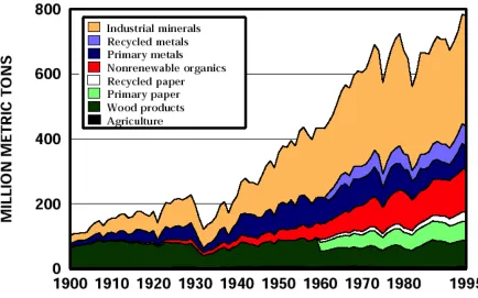
is also limited. Figure 2 shows the trend of material consumption through the years in the United
States. It is evident that the consumption has constantly been on the rise. A simple extrapolation
of this data into the future is enough to further portray this trending rise in consumption.
Industrial minerals account for the top spot in the consumption profile followed by metals (both
primary and recycled). Agricultural and other renewable resources are consumed less as
compared to the non-renewable resources, an irony considering there is a limit to the supply of
1.2 Impacts of material use
Material consumption at such a high rate has consequences on our environment.
Potential impacts include climatic changes, harmful emissions into the environment, the
depletion of our precious natural resources, constant increase in the global energy consumption.
A side-effect of such a high rate of material use is the increased energy consumption. The energy
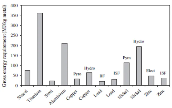
that is consumed in the production of some of these materials is quite high. Table 1 gives some
numerical values to support this claim; light metals like titanium and aluminum are the highest
energy consumers for their production cycle consuming 361 MJ/kg and 211 MJ/kg of energy
respectively (cradle to gate), followed by nickel that consumes 114MJ/kg by the flash furnace
smelting and 194 MJ/kg by the pressure acid leaking processes. Steel and lead (by the blast
furnace process) have the lowest cradle to gate environmental impacts in terms of the gross
energy required to produce one kilogram of the metal – 23 MJ/kg and 20 MJ/kg respectively.
Fossil fuels are limited and mankind should start contemplating on the long-term effects of such
a large magnitude of energy consumption. One source confirms that about 7% of the world’s
energy use goes into the metal sector (Norgate et. al., 2006). The physical properties of ores from
mining are first improved and then the ore is chemically transformed to extract metals and
produce industrial materials. This requires significant amounts of energy. Life Cycle Assessment
(LCA) methodology involves the compilation of an inventory of relevant environmental
exchanges during the life cycle of a product and evaluating the potential environmental impacts
associated with those exchanges. The full product life cycle is usually divided into the following
stages (Norgate et al. 2006): cradle to entry gate (raw material extraction and refining); entry
gate to exit gate (product manufacture); and exit gate-to-grave (product use, recycling and
also referred to as embodied energy or cumulative energy demand, which is the cumulative
amount of primary energy consumed in all stages of a metal’s life cycle (Norgate et al. 2006).
Metal Process GER (MJ/kg) GWP (kg CO2/kg)
Nickel
Flash furnace smelting and Sherritt-Gordon
refining. 114 11.4
Pressure acid leaching 194 16.1
Copper
Smelting/Converting and Electro-refining 33 3.3
Heap Leaching 64 6.2
Lead
Lead blast furnace 20 2.1
Imperial smelting process 32 3.2
Zinc
Electrolytic process 48 4.6
Imperial smelting process 36 3.3
Aluminum Bayer refining, Hall-Heroult smelting 211 22.4
Titanium Becher and Kroll processes 361 35.7
Steel Integrated Route 23 2.3
Stainless Steel
Electric furnace and Argon-Oxygen
decarburization 75 6.8
Table 1: Environmental Impacts for cradle-to-gate metal production (Norgate et al., 2006).
The energy source used to generate the electricity consumed in a particular metal production
process also influences the ‘‘cradle-to-gate’’ environmental impact of that process. This may be
illustrated by considering primary aluminum production (Norgate et al., 2006). The three main
energy sources used for generating electrical power for aluminum production worldwide in 2003
energy sources on the GER and GWP for primary aluminum production is shown in Fig. 3
[image:13.612.117.493.156.391.2](Norgate et al., 2006).
Figure 3: GER and GWP contribution of electricity sources for primary aluminum production (Norgate et al. 2006).
Apart from constant energy consumption, the global material use also brings with it
depletion and degradation of the natural resources as stated before. This depletion in natural
resources potentially affects our global climate and has negative impacts on the environment.
The biocapacity of any given area is its ability to produce or provide resources and take in the
waste. According to one source (Schaefer et. al., 2006), biocapacity is the measure of how
sustainable a resource is, with regard to the ecological footprint. Ecological footprint measures
the human demand for resources. When the ecological footprint of an area overshadows its
biocapacity, consequences of an unsustainable nature occur. This means that the resources are
are non-renewable can only be restored at regular intervals of time; some of these resources like
fossil fuels that are one of the top sources of electricity are restored over thousands of years.
With such long duration of a resource turn around, it is important that they be used very wisely.
The Earth’s regenerative ability cannot match the pace at which the resources are currently being
used. To put it in numbers, a report generated by the US Environmental Protection Agency
calculated that ‘in 2005, the global biocapacity was measured as 2.1 hectares per capita, while
the average demand or footprint per person was about 2.7 hectares’. In addition, whatever natural
resources are being used cannot be retrieved immediately and are generally returned back as pure
waste (USEPA, 2009). The growing demand of the resources and the shortage of supply are in
turn causing a rise in commodity prices.
An added consequence of the material use and the apparent energy consumption is the
global climatic changes. The increasing ecological footprint is a large factor that shapes the
global climate. As shown in Figure 3, black coal is the main source of energy for the primary
aluminum production. Burning black coal to generate electricity is a very popular option.
Burning coal releases carbon particles into the atmosphere, increasing our carbon footprint. The
carbon molecules in the air trap the heat from the sun and keep it within the atmosphere causing
global warming. There are also non carbon molecules like nitrous oxide, ozone, etc. that trap the
heat within earth’s atmosphere. The resulting warm air around us has shaped our climate to a
great extent. The leaders attending the Energy Summit of the United Nations in 1992 clearly
stated that “a principal cause of the continued deterioration of the global environment is the
steady increase in materials production, consumption and disposal” (United Nations, 1992).
According to one source, humans have consumed more resources in the past 50 years than they
worldwide consumption of raw materials doubled (USGS, June 2008). Such high rate of
consumption to match the high rate of population growth has side-effects. USEPA states that due
to this magnitude of consumption of material resources, half of the world’s tropical and
temperate forests are now gone, freshwater withdrawals doubled since 1960 and due to the ever
growing temperatures in the dry seasons; major rivers like Nile, Ganges, Mississippi sometimes
do not reach the ocean completely (USEPA, 2009). For metals, it is the mining and refinery stage
that is often very energy intensive, causing fossil-fuel-related emissions. In the case of intensive
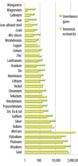
agricultural processes, growing can also be very polluting. Metals are elements and therefore not
degradable; once in the environment, they do not disappear, but accumulate in soils and
sediments. Different metals contribute to environmental toxicity in different amounts as is
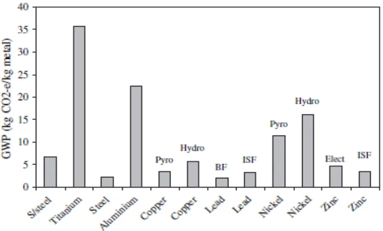
Figure 4: Contribution to terrestrial eco-system toxicity and global warming of 1kg primary metal (UNEP, 2010).
1.3 Recycling
For the factors stated above it is imperative that metals are recycled at a much larger
scale. Apart from the obvious economical advantage, the energy savings also create a strong
incentive to recycle. One of the most significant factors in the life cycle of a metal product is that
recycling has the potential to reduce production energy dramatically. Some examples include the
reduction in materials production energy consumption by 95% for aluminum, 80% for
magnesium and lead, 75% for zinc, and 70% for copper (Martchek, 2000). A report by the U.S.
Department of Energy states that “aluminum production is the largest consumer of energy on a
per-weight basis and is the largest electric energy consumer of all manufactured products”
(USDOE, 2007). Numerically, the aluminum industry in the United States consumes about 45.7
x 109 kilowatt hours of electricity which equates to more electricity than the amount consumed by the residential, industrial and commercial sectors of the U.S. economy together (USDOE,
2007). It further states the difference between the theoretical primary aluminum production
energy required and the actual energy used. On an average the minimum theoretical energy
required for the production of aluminum in the US is about 36 x 109 kilowatt hours of energy. The actual amount of energy consumed in the US is about 90 x 109 kilowatt hours (USDOE, 2007). It is clear that more energy is being used than necessary by industrial processes like
smelting, which uses about 46% percent of the total energy consumed in the US. Smelting is the
largest consumer of energy for aluminum manufacturing and is also the most technically
complex. Process heating, which is utilized in almost all aluminum production operations
amounts to about 27% of the total energy in the US (USDOE, 2007). Industrial processes like
these that consume energy at significantly higher rates than the theoretical requirements need
The practice of recovering metals for their value dates back to ancient times (Wilson,
1994) and today, the protection of earth’s resource endowments and ecosystems adds to the
incentive of recycling metals after their use. Global material consumption trends together with
the unavoidable population growth lead to an increase in the consumption of natural resources.
The inefficient use of metals and their improper disposal creates an unnecessary burden on the
non-renewable resources of the earth from which they are extracted. The dumping of used metal
has harmful effects on the environment. Some of these pollutant metals are non-degradable and
their presence in the ecosystem may jeopardize the health of all living beings (Nriagu, 1988).
One way to reduce such an atrocity to our precious ecosystem is to recycle on a vast scale. If the
sustainable use of material resources is to be achieved, a secondary production industry is very
important to be brought into the picture. In the last decade or so, secondary production of
aluminum has been quite stale as the recycling rates remain below 50% (Gaustad et. al., 2007).
One source guesses the reason for this modest increase to be the accumulation of the secondary
production of the material over time (Ayres et. al, 2000). Furthermore, metals are eminently and
repeatedly recyclable, while maintaining all their properties. Properties of a material play a
crucial role in the life of a material; in the sense that the functionality of any given material is
decided based on its properties. Their durability relative to many hydrocarbon based materials
enhances their life cycle performance. However, the persistence of metals when dispersed into
our natural environmental makes recovery and recycling particularly important. When
considering life cycle effects, recycling is critical to a sustainable future for metal products
(Martchek, 2000). Iron tops the list at about 517 MMT (million metric tons) followed by
aluminum which is about 20 MMT (Ayres, 1997). Although a significant amount of aluminum is
crucial. The current industry does not operate at the numbers that are necessary for a long term
sustainable use of aluminum. As stated before, the recycling rates are below 50% (Gaustad et.
al., 2007). Further studies have shown that out of the amount of aluminum that is recycled, 35%
consists of the end-of-life materials (Gaustad et. al., 2010). These end-of-life materials or “old
scrap” are materials that have either been discarded or have been outdated post-consumer use.
The old scrap normally comes from automotive parts, construction materials, used beverage cans
etc. and is comparatively harder to recycle than the new counterparts because of the vast mixture
of the different kinds of alloys in the scrap. The challenge arises mainly because the metal that is
to be recycled is mixed with various other materials and the contamination from these different
materials leads to unnecessary buildup of unwanted scrap in the stream. This further jeopardizes
the recycling of the metal of interest (Kim et. al, 1997 and Hatayama et. al. 2007). Recycling
barriers like the ones mentioned in the previous statements can be overcome. According to the
findings by Gaustad et. al., recycling barriers can be overcome by using strategies like “1.
Changing the form and composition of the returning scrap, 2. Changing the characteristics of the
process that converts scrap to finished goods and 3. Changing the specifications by which a
1.4 Case Study: Aluminum
It is not uncommon to know that aluminum, the youngest industrial metal is also one of
the most sought after materials. Due to its properties like ductility, malleability, conductivity and
its toughness, it matches up to iron and yet is almost 3 times as light (Boin and Bertam, 2005). It
is well known that the oxide of aluminum cannot be reduced to pure aluminum metal using either
carbon or hydrogen, that is, in a water medium. This is because aluminum is highly reactive with
the protons of water, which leads to the formation of hydrogen. The primary production of
aluminum must, thus use an electrolysis process to produce pure aluminum metal from its oxide
alumina (Al2O3) (Boin and Bertram, 2005). Charles Hall was the first person who successfully
produced aluminum through electrolysis. He started by electrolyzing aluminum salts in water.
His first attempts were unsuccessful because of the reaction of aluminum with the protons of
water, leading to the formation of hydrogen. This led him to research on a variety of other salts
that could serve the purpose of producing aluminum. When he finally passed a current through a
solution of alumina dissolved in cryolite, small traces of aluminum were found in the
electrolyzed solution. This process was adopted and has since been modified. It is now called the
Hall-Heroult process and is the most-widely used method of producing aluminum through
electrolysis (Alcoa, 1999).
Primary aluminum production starts by first converting bauxite to alumina. Bauxite is
first crushed to get uniformly sized particles that are then mixed with a sodium hydroxide
Figure 5: Crushing and grinding of the ore in the Bayer process (Alcoa, 1999).
This process discharges slurry, which is even finer in consistency and is pumped into a
digester where the chemical reaction to dissolve alumina takes place. The sodium hydroxide
solution is added as necessary to extract more alumina from the slurry and the resulting solution
is then transferred into settling tanks.
Figure 6: Digesting of the sodium aluminate solution (Alcoa, 1999).
Gravity is the main driving factor in achieving settling. The unwanted matter settles at the
dissolved alumina and caustic soda. The remaining “slurry” is dried by evaporation. In the filter,
the material that is caught is known as a filter cake; it contains alumina and caustic soda. The
filtered liquor, a sodium aluminate solution is cooled and pumped to the precipitators.
Figure 7: Settling of the mixture (Alcoa, 1999).
The large tanks known as precipitators are used for the precipitation of the pure alumina
particles. The clear sodium aluminate solution from the settling is pumped into these
precipitators with fine particles of alumina (seed crystals) to help with the precipitation process.
When the crystals form around these seeds, they settle to the bottom of the tank. They are then
removed and filtered twice before being transferred to the calcinations kilns.
Calcination is done to remove the water from the aluminum hydrate which is then
referred to as the anhydrous alumina. The crystals from the precipitation that sink to the bottom
of the tanks are moved on to the conveyer system that passes through the kilns. These kilns are
brick lined inside and heated up to a temperature of about 1100oC. The rotating kilns help in drying out the alumina evenly. The result is a fine white powder which is referred to as pure
alumina (Alcoa, Reynolds Aluminum, Aluminum Institute).
Figure 9: Calcination of the alumina hydrate (Alcoa, 1999).
Stage 2 of creating aluminum from bauxite is to convert the pure alumina to metallic
aluminum. This is achieved by an electrolysis process called the Hall-Heroult process. As
mentioned above, the Hall-Heroult process was put into practice in 1886 by Charles Hall, an
American student and Paul Heroult, a French scientist. Both made the same discovery – that
cryolite could be used to convert pure alumina into metallic aluminum. It takes place in a carbon
or graphite lined steel container. An electrical current is passed through the cryolite mixture that
contains pure alumina. This electric current, which is actually a direct current (DC) is necessary
for the transformation from pure alumina to metallic aluminum. Although the voltage for this
process is extremely low (about 5.2V), the amperage is generally very high, in the range of
100,000 – 150,000 amperes or more. The setup contains a carbon anode, positively charged
or the graphite lining of the pot. When the electric current flows from the anode to the cathode,
the carbon of the anode blends with the oxygen from the alumina. This reaction produces carbon
dioxide as the by product and molten, metallic aluminum settles down at the bottom and is then
drawn out periodically into crucibles, while the carbon dioxide escapes. A very little amount of
cryolite is lost in the process and the alumina keeps getting replenished from the containers
above the pots. The metallic aluminum collected at the bottom is now ready to be forged, turned
into alloys, or is shaped to make everyday goods like appliances, automobiles, cans, etc.
Figure 10: Electrolysis of aluminum by the Hall-Heroult process (Alcoa, 1999).
Commercially, the Hall-Heroult process is the most widely used process for primary
aluminum production. The earlier stages of the primary aluminum production are called the
Bayer process and the smelting part is known as the Hall-Heroult process (Norgate et. all, 2006).
It is the electrolysis that makes this production process one of the most energy burden-intensive
processes for materials, only second after the Becher and Kroll processes to produce titanium.
This has clearly been shown earlier in Table 1 that gives the numbers for the amount of energy
that is utilized by the production processes for various materials. As mentioned earlier, the
companies are spread across the United States where the conditions are favorable – availability
of skilled labor, the proximity to a consumer market and provisions for a highly developed
infrastructure. The United States Department of Energy wrote a report on the requirements for
aluminum production in which it claimed that hydroelectric power accounts for 50% of the
energy used worldwide for the electrolysis of aluminum. A major portion of the energy used in
the production of aluminum is related to the electricity required for the electrolysis process, i.e.
the Hall-Heroult process. Due to reasons like above, the production plants are now shifting base
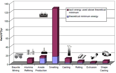
to the areas with low costing electricity. The figure below shows the tacit energy consumption of
the major processes in the aluminum production chain. Production of the primary aluminum
accounts for 87% of the energy consumed by the industry in the United States (USDOE, 2007).
Production of the secondary aluminum accounts for 4.3%, rolling makes up 3.3%, extrusion
Figure 11: Comparison of the energy consumption between the various aluminum production processes in the United States (USDOE, 2007).
It’s the industrial processes like these that make the recycling of aluminum and the
increase in the production of secondary aluminum an absolute necessity. The environmental
impacts of primary production are gargantuan and contribute to the Global Warming Potential of
a particular material. The production of metals directly and indirectly, leads to the formation of
emissions like unwanted by-products, harmful and toxic gases, unwanted solids etc. This mainly
happens during processes like mining, the consumption of raw materials and electric power,
manufacturing of reagents. In the case of aluminum, it’s the waste created during the Bayer
process and the chemical discharge during the electrolysis that is harmful to the environment.
Figures given below compare the Gross Energy Requirements and the Global Warming Potential
of energy for its production, after titanium. Similarly, it stands second to titanium on the Global
Warming Potential scale as well. Both these charts are alarming and are proof enough to
incentivize the recycling of aluminum on vast scales. Programs that improve the thermal and
electrical efficiency of the production processes, while minimizing the harmful by-products are
[image:27.612.123.482.259.485.2]to be sought after.
1.5 Barriers to Recycling:
The last two decades have seen a stagnant rate of metals recycling especially for
aluminum in the United States (IAI, 2005). The secondary recovery industry has since seen a rise
in the United States, motivated by an improving American and Asian economy. This ferrous and
non-ferrous metal recycling industry is valued at almost $60 billion in the United States and is
continuing to grow. A major trend responsible for this change is the growing demand for
products that are manufactured from recycled materials (Usifer, 2012). The outlook for this
recycling industry remains positive despite the volatile economies across the globe because of an
increase in the demand for scrap materials both by domestic and international consumers and
manufacturers (Usifer, 2012; USEPA, 2009). One source (IAI, 2009) predicts the production of
aluminum to rise to about 97 million tons by 2020 from the 56 million tons today. Consequently,
the secondary aluminum production is also expected to rise from 19 million tons as of today, to
about 32 million tons by 2020. Aluminum can be recycled over and over and over again without
the loss of its properties. The high volume of aluminum scrap is the main incentive and a major
economic impetus for its recycling.
In spite of all the advantages tied to the secondary aluminum recovery industry, there are
barriers to recycling that make it a challenging process. Firstly, it starts at the societal level due
to the lack of participation in curbside recycling. A study by (Warhurst, 2007) states that
numerous policies are in practice that indirectly prevent the growth of the secondary recovery
industry, which causes a conflict of interest for recycling materials – (1) the legality to landfill
waste is more economical than creating a funding mechanism to promote recycling, (2) funding
towards the building of incinerators, (3) manufacturing a non-recyclable product that is cheaper,
despite these, the presence of such policies makes non-recycling options cheaper and easier to
execute. The lack of incentives makes it harder for society to recycle and in turn makes it harder
to collect the materials to be recycled. Societies, communities and governments should work
alongside the industry to effectively collect and separate aluminum products.
A bigger hurdle to recycling aluminum is the compositional uncertainty in the end-of-life
material. Recycling such a complex mixture of scrap material not only becomes economically
unviable but also becomes compositionally challenging. The accumulation of unwanted material
due to contamination in both the collection and processing phases further hampers recycling
(Gaustad et al., 2010). However, from a revolutionary standpoint, we are living in a
“multi-material” world where a mixture of materials together can fulfill functions not met by just one
material. Material use intensity is also decreasing – cans get lighter, cars become smaller,
aluminum uses in transportation reduces and the foils used in packaging get thinner and thinner.
Sustainability favors such a big change in material use but it also increases the difficulty to
collect and recycle aluminum from the end-of-life products.
Another source raises the issue of saturation of sinks or “some products that can use or
absorb raw materials, for some recycled raw materials” (Gaustad et al, 2010). The only way
secondary production of aluminum can sustain is by increasing the alloy portfolio for secondary
production. In fact, other sources have already raised concerns for the limits of the available
aluminum alloy sinks for secondary production. In particular, these include aluminum castings
(Aluminum Association, AA designation 380) and wrought aluminum can stock (AA designation
3105, 3004 and 3104; Gesing, 2004; Das, 2006; Gaustad et al, 2010). Closed-loop recycling
could be a strategy if we want to avoid the unwanted accumulation of scrap from one alloy
a barrier to recycle a mixture of scrap collected from multiple classes of alloy. Another barrier is
extracting the impurities during the remelting process. A typical method to remove the impurities
in metals is by oxidation. However, there is a thermodynamic barrier to recycling which is
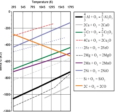
illustrated in Figure 14. The figure shows a change in Gibbs free energy as a result of
temperature for different metals (Gaustad et al., 2012). It is evident that most of the equilibrium
lines for other alloying elements have a higher Gibbs free energy than aluminum. Aluminum is
represented by the black line. This means that aluminum is oxidized before the impurities,
magnesium and calcium being the only elements that are oxidized before aluminum. A major
increase in the secondary recovery industry will only be possible if the above listed barriers to
recycling are addressed. Policies that favor an increase in recycling strategies need to be
discussed, collection of the scrap needs to be more efficient so that it favors the sorting of the
alloy types for increased closed-loop recycling. Decision makers in the secondary recovery
industry need a clear picture of the scrap use for the recycling of aluminum. Increased scrap use
Figure 14: Ellingham diagram depicting the change in Gibbs free energy as a function of temperature for various elements (Gaustad et al., 2012).
Ca Cr Cu Fe Mg Mn Ni Si C 2
2Ca + O = 2CaO
2 2
4Cu + O = 2Cu O
2
2Fe + O = 2FeO
2
2Mg + O = 2MgO
2
2Mn + O = 2MnO
2
2Ni + O = 2NiO
2 2
Si + O = SiO
2
2C + O = 2CO
2 2 3
4
2
Al + O
Al O
3
=
3
2 2 3
4
2
Cr + O
Cr O
3
=
3
295 545 795 1045 1295 1545 1795
2. Hypothesis:
As mentioned previously, one of the main drawbacks in the secondary industry is the
accumulation of the unwanted tramp elements in the scrap stream. The alloy producers make use
of blending optimization models to help quantify the inputs of raw materials (primary materials,
scrap and alloying elements) to manufacture a set of alloys within set specifications. Depending
on where someone is positioned in the secondary production industry, there are important
decisions to be made about the collection of scrap, sorting and then finally what gets allocated to
produce a particular set of alloys (Gaustad et al., 2011). The alloy producers therefore have an
important role to play in determining the actual composition of the aluminum products. Although
there are specifications that exist, determined by the Aluminum Association (AA), more
narrowly defined maximum constraints by the producers often result in reduced scrap use for the
production of a given set of alloys. This in turn, leads to an increased production cost and a
decrease in environmental savings. This paper explores the trade-offs of using a blending
optimization model where property constraints are used instead of the compositional
specifications in hopes that this will increase the scrap use, without negatively affecting the
performance metrics of the alloys of interest. Property relationships for aluminum and key
alloying compositions (magnesium, silicon, iron, copper and lithium) were statistically regressed
to create constraints for incorporation in the optimization model calculations. The main focus of
this work will be to answer the following question:
Will the replacement of the compositional specifications with property based constraints
drive increased scrap use in secondary aluminum production without negatively affecting the
3. Methodology
The main aim of this hypothesis is the substitution of property constraints for the
compositional specifications in an optimization model that aims at minimizing the production
cost of the portfolio of alloys being produced, without negatively affecting the performance of
the alloys being produced. The optimization model was created in What’s Best, an Excel based
linear optimization model. Aluminum alloys from those specified by AA were picked and used
for this thesis. Minimum and maximum production specifications were allotted for each and the
four key alloying elements (silicon, magnesium, iron and copper) were tracked. We have chosen
only to track four main alloying elements that make up the four highest compositions in any
aluminum alloy, after aluminum itself. If this work is concluded to be feasible, a larger model
can be formulated that is able to track up to twenty alloying elements. Literature research was
conducted for the relationships between the properties of aluminum and the compositions of its
alloying elements. These relationships were used for regression analysis between two variables –
the property of aluminum (dependent variable) and the composition of the alloying element
(independent variable). The regression analysis was conducted and an equation established along
3.1 Property-Composition relationships
In this study we are demonstrating the feasibility of substituting property based
constraints for the compositional based constraints in hopes that this change will increase the
scrap utilization for secondary aluminum production, without negatively affecting the
performance criteria. While compositionally based constraints were developed for blending
problems based on maintaining certain properties, many have become overly conservative in
regards to incorporation of secondary materials. The properties of a material (hardness, ductility,
malleability, conductivity etc.) are the most important factor in ensuring end-user functionality.
Properties of a material can range from chemical, mechanical, physical or electrical and the
end-user functionality can be in one of the many industries like electronics, manufacturing,
construction, transportation, aviation etc. One source gave an example of aluminum casting alloy
to be used for manufacturing a part. The different casting processes to manufacture the
aluminum alloy could be sand casting, permanent mold casting and die casting. The main
difference in these processes is the cooling rate – about 0.2 oC/s for sand casting and about 500
oC/s for die casting. The higher the cooling rate, the finer is resulting grain size which improves
yield strength, fatigue properties and wear resistance. Due to this relationship, die casting
produces the best surface finishes and better results. On the other hand, rapid cooling at such
high rates could result in a higher degree of porosity. This is a typical example of how choosing
a manufacturing process influences the properties of the finished product and its end-user
functionality (Dieter, 1997). The idea behind establishing the relationships between the
properties of a material and its composition is to make use of these relationships as constraints.
Our case study involves aluminum and hence a few select properties were first chosen
through literature research. Some of the properties of choice that were selected for this study
were – density, elastic modulus, electrical resistivity, dislocation density and melting
temperatures. These properties have well known relationships with the compositions of four
main alloying elements of aluminum – silicon, magnesium, copper and lithium.
3.1.1 Density and Elastic Modulus
The density and the elastic modulus of aluminum are influenced by the presence of
lithium in the alloy, because of lithium’s lower density of 0.53 g/cm3. “Each weight percent of Li decreases the density of Al by 3% and increases the elastic modulus by 6%” (Dieter, 1994). The
density of a material is an important characteristic because it directly relates to the mass and
volume of an object, two other important physical attributes of any material. For example, in
buoyancy, an object with a very high density will sink in to the water, whereas an object with a
low density will float. Similarly the modulus of elasticity of aluminum is just as important of a
property due to its ability to be deformed. Aluminum, as we know is extremely malleable and
ductile which makes it useful for applications of a vast variety. The density of aluminum (~ 2.7
g/cm3) is the Y-variable (the dependent) that decreases by 3% with an increase in the
composition (weight percent) of lithium in aluminum is the X-variable (the independent) (Dieter,
1994). Keeping the standard density of aluminum as the reference data point, other data points
could be calculated with every weight percent increase in the lithium composition in aluminum.
This relationship between the density and the composition can be hypothesized to be a linear
regression. Similarly, the modulus of elasticity of aluminum (~ 70 GPa) is the Y-variable (the
dependent) that increases by 6% with every weight percent increase in the composition of
elasticity of aluminum was kept as the reference data point. Figure 16 and 17 show the graphical
representation of the regression models for the density and elastic modulus of aluminum
depending on the composition of lithium.
Figure 15: Change in the density of aluminum with the change in composition of Lithium in the alloy (Dieter, 1994).
Figure 16: Elastic Modulus of Aluminum with the change in the composition of Lithium in the alloy (Dieter, 1994).
y = -‐0.0708x + 2.6833 R² = 0.99808
0 0.5 1 1.5 2 2.5 3
0 2 4 6 8 10 12
D
en
sty
o
f A
lu m in um in g /c m
3
Weight % of Li in Aluminum
Wt % vs Density
y = 5.5135x + 67.706 R² = 0.99344
0 20 40 60 80 100 120 140
0 2 4 6 8 10 12
El as % c Mo d u lu s (G P a) o f Al u m in u m
Weight % Li in Aluminum
3.1.2 Electrical Resistivity
Resistivity is one of the most important properties of aluminum because of its electrical
conductivity that make it viable for various electrical applications like electric water heater, solar
panel bodies, automotive, heat exchangers etc. The resistivity together with its lower density than
copper makes it a popular choice for long distance power lines. Though its conductivity is only
63% that of copper, its ductility and malleability make up for the drop in conductivity. The
electrical resistivity of aluminum depends on the copper content in the alloy. Copper being an
excellent conductor of electricity influences the conductivity of a material with its presence.
Literature research showed a relationship between the electrical resistivity of aluminum and the
composition of copper from one source (Reed-Hill, 1994). A statistical regression was done to
analyze the relationship between the underlying variables in question – the electrical resistivity
(the dependent) of aluminum and the composition of copper (weight percent) in aluminum (the
independent). Literature research provided the data points for this regression analysis which was
used to determine the goodness of fit for this model. The statistical significance of the estimated
relationship was found to be very close to the actual relationship based on the value of the
coefficient of determination. This relationship was then produced as a graph from the data points
in the literature research. Figure 18 shows the graphical representation of this data for the
dependent variable (electrical resistivity of aluminum) along the Y-axis and the independent
Figure 17: Electrical Resistivity of Aluminum with the change in the composition of Copper in the alloy (Reed-Hill, 1994).
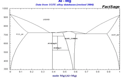
3.1.3 Melting Temperature
Many heat and thermal applications are highly dependent on this property. The melting
temperature of various alloys of Al can be changed or altered knowing its relationship with
various alloying elements present. To produce such a property-composition relationship,
different binary phase diagrams between aluminum and other alloying elements were referred to,
data points were established and a regression analysis for these data points was done. The
dependent variable here is the melting temperature of aluminum and the independent variable is
the composition of the said element in aluminum (Murray, 1985). The referenced data points
served as the basis to extrapolate the other data points and create a graphical representation of the
relationships and use the same for regression analysis. The diagrams represented mole fraction of
the element in aluminum which had to be converted to weight percent in order for the equation to
y = -‐0.0397x2 + 0.2849x + 2.6335
R² = 0.99975
2.6 2.65 2.7 2.75 2.8 2.85 2.9
0 0.2 0.4 0.6 0.8 1 1.2
El e ct ri ca l Re si s% vi ty o f Al u m in u m ( x 1 0
-‐8
ohm
-‐m
e
te
rs
Weight % Cu in Aluminum
be used in the optimization model. The mole fraction to weight percent conversion was done by
first converting the mole fraction to mass fraction and then using the mass fraction to establish
the weight percent of the element in aluminum.
Xa + Xb = 1 (Equation 2)
Where,
Xa = mole fraction of element a
Xb = mole fraction of element b.
Mass fractions can be calculated using,
γa = Xa * ma (Equation 3)
γb = Xb * mb (Equation 4)
Where,
γa = Mass of solute a in the solution
γb = Mass of solute b in the solution
ma = molar mass of a
Total mass of the solution,
(γtot) = γa + γb (Equation 5)
Weight percent,
!! = !!!
!"!∗100 (Equation 6)
!!= !!!
!"!∗100 (Equation 7)
Where,
wa = weight percent of element a
wb = weight percent of element b.
Given below are the binary phase diagrams and the statistically regressed models with the
established relationships. Table 2 gives a summary of the relationship models with their
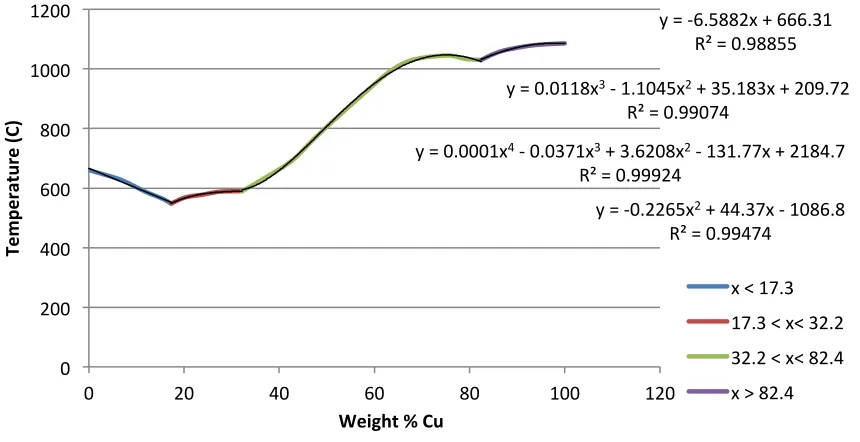
Figure 18: Al-Cu binary phase diagram (SGTE Alloy database, 2004).
Figure 19: Binary phase diagram of Al-Cu with the solid-liquid phase boundary (Murray,
1985).
y = -‐6.5882x + 666.31 R² = 0.98855
y = 0.0118x3 -‐ 1.1045x2 + 35.183x + 209.72
R² = 0.99074
y = 0.0001x4 -‐ 0.0371x3 + 3.6208x2 -‐ 131.77x + 2184.7
R² = 0.99924
y = -‐0.2265x2 + 44.37x -‐ 1086.8
R² = 0.99474
0 200 400 600 800 1000 1200
0 20 40 60 80 100 120
Temp
eratu
re (
C)
Weight % Cu
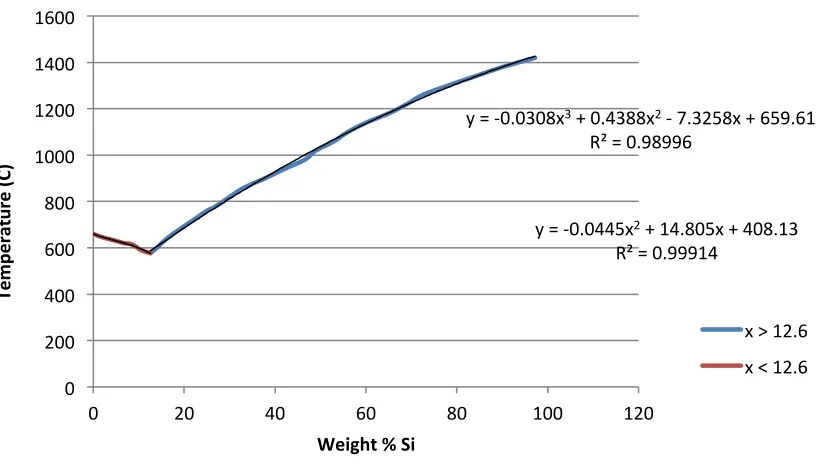
[image:42.612.94.524.419.640.2]Figure 20: Al-Si binary phase diagram (SGTE Alloy database, 2004).
Figure 21: Al-Si binary phase diagram showing the liquid-solid phase boundary (Murray,
1984).
y = -‐0.0445x2 + 14.805x + 408.13
R² = 0.99914
y = -‐0.0308x3 + 0.4388x2 -‐ 7.3258x + 659.61
R² = 0.98996
0 200 400 600 800 1000 1200 1400 1600
0 20 40 60 80 100 120
Temp
eratu
re (
C)
Weight % Si
[image:43.612.107.515.413.646.2]Figure 22: Al-Mg binary phase diagram (SGTE Alloy, 2004).
Figure 23: Al-Mg binary phase diagram with the solid-liquid phase boundary (Murray,
1988).
y = -‐5.9781x + 661.99 R² = 0.99937
y = 0.0003x4 -‐ 0.0709x3 + 5.2305x2 -‐ 164.11x + 2304.8
R² = 1
y = -‐0.0895x2 + 21.204x -‐ 576.56
R² = 0.99935
0 100 200 300 400 500 600 700
0 20 40 60 80 100 120
Temp
eratu
re (
C)
Weight % Mg
x < 35.6
[image:44.612.101.518.420.633.2]
Property Regression Equation Bibliography
Density “Each wt % of Li decreases the density of Al by 3%”
y = -0.0708x + 2.6833, x = wt% Li; y = Density of Al (Dieter, 1994)
Elastic Modulus
“Each wt % of Li increases the elastic modulus of Al by 6%”
y = 5.5135x + 67.706, x = wt% Li; y = Elastic Modulus of Al
(Dieter, 1994)
Electrical resistivity
y = 0.2451x + 2.6388, x = Wt% Cu; y = Electrical resistivity of Al
(Reed-Hill, 1994)
Hydrogen
Solubility Wt% H = exp ((-2691.96/T) – 1.32)
(Anyalebechi, 1995)
Dislocation Density
y = -1E+14x3 + 4E+14x2 – 7E+13x + 1E+14 (2nd
Order Polynomial), x = Wt% Mg; y = Dislocation Density
y = 2E+14x + 9E+13, x = Wt% Mg; y = Dislocation Density
(May et. al., 2007)
Melting Temperature (Al – Cu binary phase diagram)
For x < 17.3: y = -6.5882x + 666.31, x = Wt% Cu; y = Temperature
For 17.3 < x < 32.2: y = 0.0118x3 – 1.1045x2 + 35.183x
+ 209.72, x = Wt% Cu; y = Temperature
For 32.2 < x < 82.4: y = 0.0001x4 – 0.0371x3 +
3.6208x2 – 131.77x + 2184.7, x = Wt% Cu; y =
Temperature
(Murray, 1985)
For x > 82.4: y = -0.2265x2 + 44.37x - 1086.8, x =
Wt% Cu; y = Temperature Melting
Temperature (Al - Si binary phase diagram)
For x < 12.6: y = -0.0308x3 + 0.4388x2 - 7.3258x +
659.61, x = Wt% Si; y = Temperature
For x > 12.6: y = -0.0445x2 + 14.805x + 408.13, x =
Wt% Si; y = Temperature
(Murray, 1984)
Melting Temperature (Al - Mg binary phase diagram)
For x < 35.6: y = -5.9781x + 661.99, x = Wt% Mg; y = Temperature
For 35.6 < x < 66.7: y = 0.0003x4 - 0.0709x3 +
5.2305x2 - 164.11x + 2304.8, x = Wt% Mg; y =
Temperature
(Murray, 1988)
for x > 66.7; y = -0.0895x2 + 21.204x - 576.56, x =
[image:45.612.72.545.95.622.2]Wt% Mg; y = Temperature
3.2 Blending Optimization Model
When gauging the “recyclability” of alloys, it is imperative that a method proficient in
performing complex calculations and analysis be devised. Such a method gives a clear picture
about the potential of such alloys to be recycled in the form of secondary scrap material.
Blending optimization models are mixing software that use the physical compositional data of
any material and its alloying elements and batch them according to the specifications put in by
the user. They usually operate on compositional constraints to batch the finished alloys. Linear
programming models are used by a large number of producers to help support their purchasing
and mixing decisions (Lund et. al., 1994). The variety of secondary (recycled) materials
available for use by the producers along with the numerous elements relevant to their
composition and compositional uncertainty makes it harder to meet the specifications (Gaustad
et. al., 2007). The compositional uncertainty leads to batch plans with smaller amounts of
secondary materials. These linear optimization techniques make it easier to plan the utilization,
buying and sorting of the raw materials and also the upgrading and sorting of the secondary
materials (Cosquer and Kirchain, 2003). The optimization model used in this work in particular,
addresses the problem of mixing different quantities of raw materials (aluminum scrap, alloying
elements and pure aluminum) under certain conditions (minimum production costs,
compositional specifications and property constraints) to produce a set of aluminum alloys that is
proposed by specifying it’s compositional values. The property that a final alloy needs to have is
a linear programming optimization software, What’s Best! ® 10.0.1.3 by Lindo Systems, Inc.
was used. The mathematical definition of this model is given in equations 8-11. The objective
function in this model is to minimize the cost of production (Equation 8). Minimizing cost of
production also translates to more scrap being used to make the alloy because scraps are
generally less expensive than the pure alloying elements and primary aluminum. Equation 9
ensures that raw materials cannot be used in excess of quantities physically available. There is a
limited supply of quantities available for production and equation 9 makes sure that the
production happens keeping the quantities within the available supply limit. Equation 10 ensures
that production meets or exceeds the established target level for each product and ensures mass
balance. Each alloy produced is preset with a target production quantity. This equation limits the
quantity of the final alloy produced within the specified range, while maintaining the minimum
cost production and the limited supply of the quantities of raw material available. Equation 11
ensures that the finished alloy falls between maximum and minimum compositional
specifications. Each alloy type has compositional specifications of its alloying elements. These
specifications are limits or ranges of weight percent of alloying elements that can be present in
the alloys. It is important for the final product to meet these specifications and equation 11
Minimize: ∑CiRi (Equation 8)
Subject to: ∑xij = Ri≤ Ai (Equation 9)
Djmin≤∑xij = Pj≤ Djmax (Equation 10)
Emin < Eactual < Emax (Equation 11)
Where,
Ci = unit cost of raw material
Ri = amount of raw material, i used to produce the final alloy (in mass units)
Ai = Available amount of raw material, i used to produce the alloy (in mass units)
Djmin = Min amount of the final alloy, j demanded (in mass units)
Djmax = Max amount of the final alloy, j demanded (in mass units)
Pj = Amount of the final alloy, j actually produced.
Emin = Min amount of an alloying element supposed to be present in the final alloy
Emax = Max amount of an alloying element supposed to be present in the final alloy
3.3 Data and Assumptions:
Optimization models are methods used by many secondary alloy producers to determine
the recyclability of any given set of scraps. Closed-loop recycling has been a recurring topic in
this work as it is known to be the first choice when trying to recycle any aluminum alloy. Closed
loop recycling means gathering scrap from the same industry or a class of alloy that is needed to
be produced. For example, to recycle the aluminum used in containers and packaging, scrap from
the same industry is collected and recycled to produce alloys that are compositionally close to
those that are used to serve the containers and packaging industry. However, secondary alloy
producers need to be able to formulate decisions based on alloys that are produced from a wide
variety of scrap portfolios. In this work, we have attempted to accomplish this by creating a
model that explores mixing raw materials (aluminum scrap, alloying elements and pure
aluminum) in order to create a new set of alloys under the property constraints put forth in the
model. The scraps chosen to be used in this model represent the three major industries globally
where aluminum is used. These are – containers and packaging, automotive and transportation
and building and construction. Used beverage cans (UBC) are the scrap aluminum collected from
the containers and packaging industry and mainly consist of the alloys that serve this industry.
The transportation and automotive industry comprises of mixed auto castings and Cu-Alum
radiator scrap. These scraps are predominantly from automotive industry as supposed to the
general transportation industry. Wire and cable scrap, mixed turnings and litho sheets are a part
of the building and construction scrap. The compositional specifications for this scrap set were
established by the European Union standards (ECS 2003). Other alloying elements like iron,
magnesium, silicon etc. are also a part of the alloy composition in varying amounts in order to
compositionally different than alloy 2024, even though both alloys belong to the 2xxx series. For
the sake of this thesis work however, we decided to track only four of the main contributing
alloying elements that make up any given aluminum alloy – silicon, magnesium, iron and
copper. These four elements have the highest contributions towards an aluminum alloy apart
from aluminum. The prices for this scrap set including the alloying elements were estimated
from online sources (Scrap Register, 2014) and do not represent data from any particular firm or
organization; these are general scrap prices widely used across the metal.
Alloy Minimum/Maximum
Production
Requirements Si Mg Fe Cu
2219
Min 10000 0 0 0 0.058
Max 100000 0.002 0.0002 0.003 0.068
3004
Min 20000 0 0.008 0 0
Max 120000 0.003 0.013 0.007 0.0025
4032
Min 15000 0.11 0.008 0 0.005
Max 100000 0.135 0.013 0.01 0.013
5052
Min 25000 0 0.022 0 0
Max 100000 0.0025 0.028 0.004 0.001
6061
Min 25000 0.004 0.007 0 0.0015
Max 150000 0.008 0.012 0.007 0.004
7075
Min 15000 0 0.021 0 0.012
[image:50.612.60.555.304.583.2]Max 100000 0.004 0.029 0.005 0.02
Table 3: Production requirements of the final alloys (AA, 2007).
To avoid any problems arising from a restricted supply of raw materials, we assumed that
all the raw material and scraps were available in unlimited quantities. For the sake of the
optimization model in this work, however, the available scrap had to be quantified. The final sets
3004 and 6061 which had a maximum production scale of 120,000 lbs. and 150,000 lbs.
respectively, totaling the final production portfolio to 670,000 lbs. for the entire set. Since we
calculated the final results assuming an unlimited supply of the raw materials, they are also
independent of the production scale. The final sets of alloys to be produced were selected from
the six predominant series of aluminum alloys as described and set by the Aluminum Association
(AA). The final set of alloys to be produced were – 2219 from the 2xxx series, 3004 from the
3xxx series, 4032 from the 4xxx series, 5052 from the 5xxx, 6061 from the 6xxx series and
finally, 7075 from the 7xxx series. We specified a minimum and a maximum amount of each
alloy to be produced to show a realistic approach to the mixing model evaluation. A minimum
production value of the alloy was specified to make sure that all the alloys were produced. Pure
4. Results and Discussion
4.1 Base Case Results
The optimization model evaluates the potential of the scrap material utilization in
producing a set of new aluminum alloys (2219, 3004, 4032, 5052, 6061 and 7075). These sets of
alloys are currently available as end-market alloys with specifications set by the Aluminum
Association (AA).
2219 3004 4032 5052 6061 7075
UBC 0 20000 13198 12326 24955 14667
Mixed auto castings 0 0 0 0 0 0
Cu- alum radiator 2255 0 157 0 0 0
Wire and cable scrap 444 0 0 12294 0 0
Mixed turnings 0 0 0 0 0 0
Litho sheets 2639 0 0 0 0 0
Si 0 0 1645 0 45 0
Mg 0 0 0 380 0 174
Fe 0 0 0 0 0 0
Cu 0 0 0 0 0 160
[image:52.612.66.567.246.501.2]Al 4661 0 0 0 0 0
Table 4: Primary results of the optimization model showing the amount of scrap and alloying elements used for each alloy (in lbs.)
Table 4 shows the trend in the amounts of scrap used in the production of each individual alloy.
As seen in table 4, different alloys require different quantities of scrap for their production. The
potential of an alloy to use scrap for its production is called its recycle friendliness (Gaustad et.
al, 2010). Scrap prices are lower than the primary alloying elements which drive the
minimization of the production costs. Consequently, the objective function of this model was to
produced with a 100% scrap, making it the most recycle friendly alloy. Within its 100% scrap
use, it is interesting to notice that all of its scrap came from one source – UBC (used beverage
cans). This aligns with the uses of most of the alloys in the 3xxx series as their major use is in the
containers and the packaging industry. One source confirms that the three main alloys used in the
packaging industry are the 3000 series with manganese being its main alloying element, the 5000
series with magnesium being the man alloying element and the 1000 series which is a high purity
aluminum alloy with the alloying elements making up only 1% of the total composition and the
[image:53.612.108.514.344.566.2]rest 99% is pure aluminum (Terukina, 2013).
Figure 24: Percentage of scrap use for each alloy.
Used beverage cans make up a majority share of the scrap available in the United States (IAI,
2009). This is evident from the scrap use numbers in Table 4 as most of the scrap that is used to
produce each alloy comes from the UBCs. Except 2219, all the other alloys use at least 60% or
0 20 40 60 80 100 120
2219 3004 4032 5052 6061 7075
Sc
ra
p
u
se
(
%)
Alloys