Theses Thesis/Dissertation Collections
8-2016
Validating the Operating Window Concept for
Robustness on a Circuit Board Stencil Printing
Process
Wagner Pereira Romito [email protected]
Follow this and additional works at:http://scholarworks.rit.edu/theses
This Thesis is brought to you for free and open access by the Thesis/Dissertation Collections at RIT Scholar Works. It has been accepted for inclusion in Theses by an authorized administrator of RIT Scholar Works. For more information, please [email protected].
Recommended Citation
by
Wagner Pereira Romito
Thesis submitted in partial fulfillment of the requirements for the
Degree of Master of Science in Manufacturing and Mechanical System Integration
Rochester Institute of Technology
College of Applied Science & Technology
Department of Manufacturing and Mechanical System Integration
College of Applied Science & Technology
Master of Science in Manufacturing and Mechanical System
Integration
Thesis Approval Form
Student Name:
Wagner Pereira Romito
Thesis Title:
Validating the Operating Window Concept for Robustness on a
Circuit Board Stencil Printing Process
Thesis Committee
Name
Signature
Date
Dr. James Lee
Chair
Dr. Robert Garrick
Committee member
“O objetivo fundamental dos sonhos não é o sucesso, mas nos livrar do fantasma do conformismo.”
I am thankful to everyone who contributed, directly or indirectly, with the development of this research.
I acknowledge my advisors for the opportunity and support that ledge to the completion of this project.
To the MMET department and all the faculty members that provided the tools to build and improve my knowledge.
To the Rochester Institute of Technology (RIT) for the amazing reception and structure that enabled the development of this research in a soundly manner.
I would like to thank CAPES/CNPq for funding my master program under the Brazilian Scientific Mobility Program (Ciências sem Fronteiras), process number 88888.076031/2013-00.
To Jeffrey Longville and Tayler Swanson from the CEMA lab, for supporting me on the experimental phase of this research.
I am thankful to QVI, specially Ken Sheehan, for opening the doors of their company and providing access to their metrology machinery.
I specially thank my friend and partner Ana Carolina Pessôa, to encourage me to embark on this journey.
To my grandparents, because they have not measured efforts to always give me the best education.
To all my family for all the love and support that was the foundation that enable me to pursue my dreams.
And finally for all my Brazilian friends that shared these two years as a great family.
The lifecycle of a system is dependent on the system design. However, the concern with quality
has been stressed mostly during its production and use. The understanding of the system
variability generated by noise variables shifted the quality focus to the design phase. The
development of robustness early on the system lifecycle increases the system reliability through
its entire life cycle. Although the robust design approach developed by the Taguchi methods
application had a great contribution to this philosophy, there is much criticism of this
methodology. One alternative to the Taguchi method is the Operating Window methodology.
Its application has successfully been demonstrated as a substitute for the Taguchi methods,
especially when the response is not quantitative. However, most of the examples were used
repeatedly and the steps on the application of the methodology have not been well detailed.
Therefore, this project had the objective of developing a unique application of the methodology
with a simple approach. Moreover, with the implementation of the methodology, the project
aims to identify the difference between a design with a wide output data distribution and a design
with a narrow distribution. The methodology followed the Operating Window methodology
steps, applying it to a circuit board printing process. The results have shown that it is possible to
have a relationship between the Operating Window range and the distribution variation from the
Table of Contents
Introduction ... 1
Literature Review ... 4
Robust Design ... 5
Product lifecycle. ... 6
Taguchi methods. ... 7
Noise. ... 10
Tolerance Design ... 11
Operating Window ... 13
Previous application. ... 17
Failure Boundaries ... 18
Failure modes. ... 18
System physics. ... 19
Project Objectives ... 20
Methodology ... 21
Materials ... 23
Stencil Printer. ... 23
Measurement. ... 29
Operating Window Methodology ... 31
Identifying the operating window factor. ... 31
Failure rate and noise level. ... 32
Designs selection. ... 33
Constraints. ... 37
Identify the operating window. ... 38
Robustness Developing Cycle ... 41
Noise level increase. ... 41
Robustness and time trade-off. ... 42
Analysis and Results ... 43
Operating Window Factor ... 44
Noise Level ... 47
Design Selection ... 47
Experiment. ... 47
Identify the Operating Window ... 52
Conclusions ... 58
References ... 62
Appendix A ... 68
Appendix B ... 77
Appendix C ... 79
Appendix D ... 81
List of Figures
FIGURE 1. PRODUCT LIFECYCLE COST ... 6
FIGURE 2. METHODOLOGY FLOWCHART ... 22
FIGURE 3. STENCIL PRINTER ... 24
FIGURE 4. STENCIL PRINTER FLOWCHART ... 25
FIGURE 5. STENCIL PRINTER DIAGRAM ... 26
FIGURE 6. SOLDER PASTE PRINTING PROCESS ... 27
FIGURE 7. STENCIL PRINTER VARIABLES ... 28
FIGURE 8. SMARTSCOPE QUEST 650 ... 31
FIGURE 10. PRINTING FLOW ... 37
FIGURE 11. MINIMUM PRINT DEPOSIT VOLUME ESTIMATION ... 40
FIGURE 12. PROGRESSIVE DEVELOPMENT ... 41
FIGURE 13. GAGE R&R COMPONENTS ... 46
FIGURE 14. BOXPLOTS DIAGRAM OF MAIN FACTORS ... 48
FIGURE 15. BOXPLOT DIAGRAMS WITH FACTORS LEVELS ... 49
FIGURE 16. HISTOGRAMS ... 51
FIGURE 17. OPERATING WINDOW EXPERIMENT RESULT ... 56
List of Tables
TABLE 1.TAGUCHI METHOD GENERIC EXAMPLE ... 9
TABLE 2.DESIGN FACTORS AND THEIR LEVELS ... 35
TABLE 3.APERTURE SIZE ... 45
TABLE 4.GAGE R&R VARIANCE COMPONENTS ... 46
TABLE 5.GAGE R&R PROCESS VARIATIONS ... 46
TABLE 6.MINIMUM SOLDER CALCULATED VALUES ... 50
TABLE 7.SELECTED DESIGNS ... 52
TABLE 8.HIGH TE VARIATION DESIGN RESULTS ... 53
Table of Abbreviations
AR Area Ratio
CEMA Center for Electronics Manufacturing and Assembly
CAD Computer-Aided Drafting
FAMe Failure Amplification Method
FTA Fault Tree Analysis
Gage R&R Gage Repeatability and Reproducibility
LD50 Half of the Lethal Dose
in Inches
nl Nanoliters
lbs Pounds
PCB Printed Circuit Board
SMT Surface Mount Technology
TRIZ Theory of Inventive Problem Solving
TE Transfer Efficiency
Validating the Operating Window Concept for Robustness
on a Circuit Board Stencil Printing Process.
Introduction
Quality control is performed to guarantee that the process will produce products as
expected. The process is controlled as to not allow the production of products outside the
customer requirement limits. Although final inspection is known to be used as a ineffective
attempt to avoid bad products from being delivered to the customer (Juran & Godfrey, 1998),
companies still use this quality assurance procedure alone. However, the main quality efforts
should be focused on assuring that the process is capable of producing within the customer
requirements during its life cycle. The reason that final inspection should be avoided is that it is
performed at the end of the process, when the product has already been produced and the defects
have already been generated at some earlier point in the process. This means that if any fail to
meet the customer specification is detected at this point, it will result in more costly production
waste. The costs of rejecting a product after it has been produced are greater than the cost of
preventing the nonconformance (Juran & Godfrey, 1998; Crosby, 1979). Moreover, when this
inspection system fails and a defective product is not detected, the consequences are even
greater.
As process capability is mainly a measurement of the effects of variability on the process,
efforts should be made to reduce the process variability (Gryna, Chua, De Feo, & Juran, 2007).
An alternative approach to controlling variability during the entire life cycle is to engineer the
product or process to be robust enough to account for this variability (Clausing, 2004). Although
effective approach (Clausing, 2004). Quality efforts in companies have been developed to fix
problems related to production. Programs such as Six Sigma have been heavily developed to
control the occurrence of production problems (McClusky, 2000). Although the success of these
methodologies has been proven, the design of a process resistant to noise would eliminate the
need for such process control approaches. In other words, the lack of process robustness creates
the necessity to develop problem-solving programs such as Six Sigma in order to reduce the
effects of noise variables on the production system (Clausing, 2004).
Solving product problems and solving process problems are different in nature and can
lead to different consequences. In many cases, even when a process is not effective, it can be
adjusted and changed before the final product is produced. However, a product cannot be fixed
after it was already delivered to the customer without greater consequences (Feigenbaum, 1991).
This is true as customers expect the product functionality to be reliable during its entire life cycle
(Yang, 2007). The consequences could be financial or related to customer satisfaction (Juran &
Godfrey, 1998). Satisfaction of the customer is the key factor to a company’s success. Because
of the need to achieve customer satisfaction, products have to be designed to maintain its
performance as expected during its entire life cycle (Bergman, de Mare, & Svensson, 2009;
Schenkelberg, 2013). This is achieved by designing performance robustness into the product.
Robustness is achieved by making a system insensitive to noise effects. The introduction
of the robustness concept into the design phase is a key to designing a system able to meet
customer requirements under different operating conditions (Clausing, 2004). Robust design can
be useful for both product and process development. Many times in new product development,
the process is not capable of yielding the expected results to produce the product under
product characteristics exceed the existing process capability. However, these changes might
increase the development cost and time. In addition, machinery restrictions might hamper the
product development when the product characteristics exceed the machine limits. To assure
quality, things have to be done right from the first time (Crosby, 1979). This suggests that a
process needs to be developed considering all possible applications during its life cycle. A
process robust to changes on its main functions is necessary to enable the use of new
configurations on the product development procedure.
The robust design methodology gained large scale adoption through Taguchi’s
development and implementation of an experimental design methodology often referred to as
Taguchi methods (Roy, 2010). However, Taguchi’s approach has also been critiqued (e.g. Nair
et al. 1992) and new methodologies have been developed to address the problems identified in
the Taguchi methods. The Operating Window concept is one example. Although the Operating
Window methodology has been studied on some examples (Fowlkes & Creveling, 1995; Mori,
1995; La Vallee, 1992; and, Peace, 1993) there is still a need to further develop the methodology.
Among these are the need to better define the steps to apply the methodology in practice and the
need to develop more examples of its application. For instance, the paper feeder subsystem (La
Vallee, 1992) and the wave soldering process (Peace, 1993) are the two main examples that have
been used in the operating window research. Considering the importance of developing
robustness of a system early in its development and the problems identified with Taguchi
methods, this research will apply of the Operating Window methodology to the development of
process robustness.
In this work, the Operating Window methodology was applied to test the hypothesis that
narrower distribution. A large variation means that the specific configuration presents small
capability of performing under acceptable conditions. On the other hand, configurations with a
small variation have a greater probability of meeting performance specifications. Therefore,
designs with smaller variations should outperform designs with large variations in terms of
capability. In addition, designs with narrow distributions should be less sensitive to noise
effects; hence these designs should have a greater level of robustness when compared to designs
with wider distributions.
The remainder of this thesis is organized as follows: Literature Review, Project
Objectives, Methodology, Analysis and Results, and Conclusions. The first Chapter will
summarize the literature used as a source of knowledge for the development of this study. It
contains the theoretical framework that guides and justifies this research. And, it will identify
the gaps on previous research. The second Chapter will propose the objective to fill the
identified gaps. The third Chapter presents the methodology used in the project. It covers the
definition of the study universe, the instruments used, how the data was collected and analyzed,
as well as its limitations. It will explain how the objectives will be achieved. The fourth Chapter
will present the experimental results and findings. Finally, the fifth Chapter presents the
conclusion of the research, summarizing the findings and learnings as well as presenting
suggestions for future studies.
Literature Review
In this section, a review of related literature will be presented. First, an overview of
robust design will be presented, which will describe its role in the product life-cycle, present a
review of Taguchi methods and the critical role that the noise plays. In addition, since the
review of tolerance design is included. Finally, a detailed review of the Operating Window
concept is included, which includes its previous applications, and the definition of failure
boundaries through failure modes analysis and the analysis of the system physics.
Robust Design
Robustness is defined by Clausing (2004) as the system’s capacity to perform as expected
even under the effects of noise factors. A new system has to be able to produce the same results
in different operating conditions. This adaptability is defined as robustness and is achieved
through the adjustment of the technology variables (Taguchi, 1993). The concept of robustness
represents the intrinsic system setup that allows the system to function as expected even under
the presence of some disturbance that could harm the system operation. A process is considered
robust when changes in the production environment do not affect the production quality. The
process continues to produce within the tolerance limits even when those changes are present.
Systems are developed based on previous systems performance. Incremental changes are
implemented to overcome identified problems on previous versions by adding new features to
the system. This problem-solving approach is a major problem of the traditional system
development. It is a good approach to solve emergency or small problems but it fails to
eliminate the root cause of the problem. Robustness is the right approach to eliminate the
problem by reducing variance (Clausing & Fey, 2004). Problems are consequences of the
system functions variance. Large variations generate system malfunctions. The development of
system robustness reduces the variance and, consequently, reduces the probability of problems to
occur. Robust design methods to reduce variance have had great success to improve reliability in
addition to quality and consequently this leads to customer satisfaction (Meeker and Escobar,
Robustness is part of reliability improvement of a system by avoiding failure modes and
it should be developed early in the design stage when modifications are cheaper (Clausing, 2004)
and less restricted. Robust design aims to optimize the relationship between control variables
and output responses (Mori & Tsai, 2011) it enhance a system’s quality and reliability, reduces
warranty costs and customer service costs, speeds up the time to market, and reduces
development costs (Clausing & Fey, 2004).
Product lifecycle. The design process is a phase of the product lifecycle as is shown in
Figure 1. The design phase is a systematic process that conceptualizes a new system.
Innovations or customer needs are translated into the activities necessary to produce the new
system. The design phase identifies the real market needs, defines the system’s functions and its
requirements, defines the product specifications, and identifies the process variables necessary to
[image:18.612.157.455.404.591.2]produce that product (Wallace & Clarkson, 1999).
Figure 1. Product Lifecycle Cost. This figure illustrated the product lifecycle phases and costs.
Adapted from" Systems engineering and analysis." by Blanchard, B. S., & Fabrycky, W., 2010.
The concern with fast customer satisfaction prejudices the design phase of a system
changes are not fully analyzed. This lack of proper planning generates problems that will need
to be fixed late in the development phase. The design decisions need to be based on the entire
system lifecycle (Blanchard & Fabrycky, 2010).
The design phase enables development cost reduction. Figure 1 shows that changes early
in the design phase are less expensive to implement and have a big impact on the reduction of the
system life cycle cost. This is true because late in the development process, the decisions that
were taken earlier committed to these downstream costs (for example, an inexpensive yet
unreliable design selected early in the design phase, could lead to a larger number of product
development testing failures, manufacturing defects and field failures). This situation
emphasizes the importance of early design decisions. However, Figure 1 shows that current
practices of delaying design decisions and cost commitment can increase the system
development costs (Blanchard & Fabrycky, 2010).
In addition to the life cycle cost reduction opportunity, the development of robustness
early in the design phase reduces the time of subsequent activities and consequently the product
time-to-market. However, some concern has to be taken not to spend too much effort achieving
robustness and missing the time-to-market (Clausing & Fey, 2004).
Taguchi methods. Product development used to follow a trial and error approach (von
Hippel, 1998). On a trial and error practice, robustness was improved by identifying how to
break a component, then making the component harder to break. Failure was identified and
typically, a one factor at a time approach for experimentation was followed. Several trials were
necessary for this approach and the performance of output response was limited to a target
Fey (2004), system robustness is achieved more quickly by analytical methods as opposed to
experimental methods.
Taguchi (1986) was the precursor of this philosophy with the development of methods to
increase system robustness. The Taguchi method is defined by two-step to maximize the signal
to noise ratio in order to meet the customer’s requirements. The first step minimizes the system
variability under operating conditions, making the system robust to noise. It is achieved by
varying the system variables in order to achieve the appropriate signal to noise ratio. After the
system is made robust, the second step consists of bringing the parameters close to the values
specified by the customer. Taguchi (1993) defends that is it not possible to focus only on the
customer requirements. Once the system is under operating conditions it has to be robust to
yield the expected result that was obtained under controlled conditions.
As it is explained by Roy (2010), the Taguchi method uses orthogonal arrays to create
experimental protocols that facilitate the analysis of system performance. It is composed of an
inner array that contains the system control parameters levels used in the experiment and, if the
noise variables have been identified and can be controlled, by an outer array with the noise
variables levels. Table 1 shows an example of orthogonal arrays. The inner array is often a
fractional factorial array used to estimate the main effects, as these types of factorials have
confounded factors in its alias structure. This mean that the it is not possible to estimate each
factor effect separately. The estimated effect will be the sum of the effects of the two or more
factors that are considered confounded. The relations of all factors are defined on the alias
structure. Each row of the inner array represents a system configuration that will be used to run
column of the outer array represents the noise condition in which the runs will occur. The
analysis is made with these responses’ means and by a signal to noise ratio (Roy, 2010).
Table 1
Taguchi method generic example.
Runs
Inner Array Outer Array
Mean Response Signal to Noise Ratio Factor 1 Farctor 2 Factor 3
Response values under Noise condition 1 Response values under Noise condition 2
1 1 1 2 10 20 15 6.53
2 1 2 1 13 23 18 8.12
3 2 1 1 14 26 20 7.45
4 2 2 2 5 11 8 5.51
The signal to noise ratio is a measurement of variability created by the noise variables as
can be seen in Table 1. This performance measurement is the ratio of the quality factor effect to
the noise factor that influences the signal. The use of the signal to noise is made through a
logarithm transformation as can be seen on Equation 1. The measurement efficiency is improved
by the logarithm transformation as it increases the additivity of the input variables over the
output response (Mori & Tsai, 2011). The signal to noise ratio is a measurement that can be
applied to different types of technology but it does is not a comparable measurement (Taguchi,
1993). It is not possible to state that a product is more robust than a different product by just
comparing their signal to noise ratio.
S/N = 10 log +,
Taguchi (1986) applied a quantitative method to deal with robustness through the signal
to noise ratio. Although the Taguchi approach have the advantage of relying on quantitative
data, in some circumstances, the collection of continuous data is not possible or not affordable.
Sharma and Cudney (2009) identified that the methodology developed by Taguchi (1986) was
not balanced. In terms of the operating window, the methodology applied distinct statistical
transformations at each of its limits, generating a higher impact on the lower limit. Because of
this problem a new methodology was proposed to provide more realistic outcomes to the
optimization process. Joseph and Wu (2002) considered that the model developed by Taguchi
(1986) was functional under restricted assumptions. A more flexible model was developed by
the application of general linear functions and a two-step approach for optimization.
Noise. During the innovation process, a new system might work well in a laboratory
environment, however, its performance changes during production, because of uncontrollable
variables inherent in the process. The changes in the product performance during production that
differ from those in a controlled environment (typical under ideal conditions) is caused by noise
(Clausing & Fey, 2004). Noise is defined as the non-controllable variation in a functional
parameter, critical for the system performance. (Clausing, 2004).
The function of a system can be divided into two parts, first is the optimal function of the
system defined as useful part. The second is the effects of noise variables over the function
defined as harmful part (Taguchi, 1993). The noise increases the probability of a failure mode to
occur (Clausing, 2004) as it increases the variation in the system performance. Variation in the
product characteristics are a reflection of noise. These variations include (Clausing & Fey,
• Environmental variation:
o External environmental variation
o Customer-use profile
o Interactions with other subsystems and components.
• Variations in the product characteristic:
o Variations in production: Noise to the designers. Variation in production affects
the system performance. However, if the system is robust, the production
variations will not have a high influence on the system performance.
o Variations as the result of time and use, it includes wear and deterioration.
Noise is the cornerstone of the operating window methodology. It is applied as a factor
to increase the system’s variation and is used to measure system’s robustness through the critical
parameter variation (Clausing, 2004). Armillotta and Semeraro (2013) also highlight the
importance of studying functional requirements in the presence of noise early in the design
phase. Functional Noises are defined as functional variables that control the physics of the
product main functions. The system is made more robust by controlling these variables
(Clausing & Fey, 2004).
Tolerance Design
Tolerances are the limits that allow a parameter to assume different values (Creveling,
1997). The nominal value of a parameter is usually defined during the design stage. However,
as Bernardo and Saraiva (1998) suggest, this definition often ignores the control phase that will
use the defined value. Ignoring the parameter control by defining a single nominal value instead
of a variation range, the defining effort fails to address noise that will be present in operation
value. Creveling (1997) argues that the tolerance limits should be conceived in the design stage,
based on the customer perception or the system function.
The specification of tolerance limits has the objective to protect a system’s main function
from deviating from its expected outcome. For example, to prevent the system from operating
outside its specified limits and generating safety issues. In other words, the nominal value is
seen as a target but there is a range of values that yields acceptable quality levels. The threshold
of this interval is identified by changing the systems variables until a failure occur (Taguchi,
1993). The tolerance design decision, in Taguchi’s (1993, pp. 39) opinion, should be “based on
the trade-off between the average quality loss function and the average cost of products”. The
tolerance interval of control variables reduction cause the control cost to increase (Bernardo &
Saraiva, 1998).
Often a safety factor is necessary to assure that the variation during production does not
let to the production of a defective system (Taguchi, 1993). The necessity of this safety factor
exists because the product development process occurs in a controlled environment. When the
developed system is placed under operating conditions, it experiences the effects of noises that
were not present in its development. Such noises can make its functions’ variability increase to
levels that might take it outside of its requirement limits.
Tolerances are identified taking into account variations from the mean value of a specific
design parameter. However, there is a need to account for all operation factors inherent to the
system when the design parameter variance is defined (Armillotta & Semeraro, 2013). The
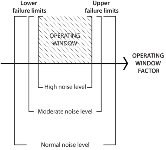
Operating Window
Herron, Hodgson, and Cardew-Hall (1998) defined operating window as the operating
limits that consider the variables of a process as a single system. In other words, the operating
window can be thought as the boundaries of a system a critical parameter where after, failure
modes are more likely to occur (Joseph & Wu, 2002). Clausing (2004) identified the operating
window as a robustness metric that is easily measured in practice and that is directly related to
the prevention of a system’s identified failure modes occurrence. Operating window is a range
of values that the operating parameters meet the specified functional parameters (Armillotta &
Semeraro, 2013) yielding the best results in economic and quality terms (Bernardo & Saraiva,
1998).
The operating window upper and lower boundaries are defined as failure limits. A two
dimensional operating window is bounded by failure modes on both sides (Joseph & Wu, 2002).
For this reason, a system’s critical parameter has to avoid these boundaries. The critical
parameter has to be small enough to reduce the probability of failure from the upper limit, but
has to be large enough to minimize the probability of failure from the lower limit (Sharma &
Cudney, 2009). The critical parameter can safely obtain values inside this range. However,
mostly due to noise, variability may increase the probability of failures modes. Sharma &
Cudney (2009) explains that one can increase the range of values that the critical parameter can
obtain by widening the operating window limits. This fact makes the systems more robust due
noise variation. So, the larger the operating window, more robust is the system.
The objective of the operating window approach is to make the product robust early in
the design phase by inducing high failure rates through changes in operating parameters and the
executed late in the development phase where the ability to make changes is restricted and a
large number of trials are needed to assess small failure rates. In response to that, the operating
window uncovers robustness problems early in the design phase with fewer trials. This is
possible by inducing high failure rates early in the design phase and using noises factors to excite
the failure modes. The large amount of noise applied, makes the system development to
consider a scenario closer to the real operating environment (Clausing & Fey, 2004).
The difference is that the product will be developed under the effects of noise instead of
dealing with this effect only in the production phase and having a high chance of failure
(Clausing & Fey, 2004). Early in the product development phase, the systems are typically
developed under controlled conditions just to prove that its performance can be superior to a
previous model. However, with the introduction of the operating window concept, what will be
discovered is that the operating window is narrow or even negative as the system will be
vulnerable to failure modes in operational conditions. But it is the early introduction of this
noise and the excitation of these failure modes that enables the system control variables to be
defined and enables learning from failure, which ultimately leads to a more robust product. This
increase in robustness is directly linked to the opening of the operating window (Clausing & Fey,
2004).
The system operating window is defined after the understanding of the system function,
its failure modes, and the noise that generate them. Clausing and Fey (2004) explain the process
by first setting the system with its best know operating parameters. The second step consist of
inputting a fixed noise variable and adjusting the operating window variable to have a high
failure rate, generally, 0.5. The process is repeated for the other side of the operating window.
window is opened, the noise level is increased to further improve the operating window. The
best approach is not yet defined. But the main concept behind the operating window approach,
independent of the method used, is the understanding of the system physics (Clausing & Fey,
2004).
The identification of the operating window is a quite simple task given a single or two
system critical parameters (Armillotta & Semeraro, 2013; Clausing, 2004). However, a
multidimensional set of requirements increases its complexity becoming a difficult task for
product designers (Armillotta & Semeraro, 2013). Operating window for a single critical factor
is easily defined and achieved. However, systems usually have more than one critical factor but
few examples have been studied (Clausing & Fey, 2004).
The development of robustness through the operating window has to be gradual. Starting
with a moderate level of noise then increasing after the operating window is found and expanded
for each level. The expansion of the operating window is made based on the system control
parameters. This approach would make the system robustness to constantly increase for the
initial noise level (Clausing, 2004). The result of the operating window process is the definition
of the set of design parameters that yield the best result to the system and its tolerances. The
level of these parameters are set as a requirement for the next activities until the final commercial
concept is developed (Clausing & Fey, 2004).
Compared to Taguchi (1986) approach, the operating window is easier to be applied by
the development team as it is more intuitive in terms of engineering (Clausing & Fey, 2004).
The operating window is developed exploring the system physics and allows the robustness
development without quantitative experimental results. Taguchi (1993) stated that the operating
experimenter to obtain more information, categorical variables are easier to obtain and can be
converted to other measurements as pecuniary (Joseph & Wu, 2004).
Although the measurement of the system robustness is better achieved through the
identification of a functional attribute, it is a difficult task to identify or measure the appropriate
functional attribute (Joseph & Wu, 2002). Joseph and Wu (2002) identified the use of the
operating window as an opportunity to deal with the functional attribute problem by identifying a
single “operating window factor” to define the limits of which failure modes are likely to affect
the system. Because the operating window defines the limits where a systems critical parameter
could vary without failures, to deal with noise, it would be reasonable to think of enlarging those
limits and make the system more robust (Joseph & Wu, 2002).
The Taguchi method first identifies the value that yields a better outcome in terms of
robustness then the tolerances are calculated based on this value. The operating window method
has the opposite sequence. It first identifies the thresholds values for the operating window.
After the limits are identified, the set point is defined taking into consideration the distance from
the limits and the severity of the failures at each boundary. The identification of the operating
window generally occurs by looking at the thresholds separately. One signal to noise ratio is
developed for each limit. For the lower boundaries it assumes a smaller the better property and
for the upper boundaries a large the better characteristic. The operating window signal to noise
ratio is the sum of the thresholds signal to noise (Taguchi, 1993).
The operating window is identified by Taguchi (1993) as a methodology to develop
robustness in a new technology in an efficient way. It allows improving robustness in a reduced
quantity of development cycles and cost compared to traditional approach. Clausing (2004)
importance than the method used to identify the range of control parameters where the higher
level of robustness is achieved.
Previous application. Many industries do not have full knowledge of how their
production systems work and this knowledge is usually concentrated within employees with
more experience. However, in a dynamic environment with changing product needs, these
experienced employees also face a lack of knowledge to adjust the machines to produce new
products (Herron et al., 1998). Herron et al. (1998) identified the need to understand a system’s
operating window and to develop an interaction framework. The employees that setup the
machine, uses the operating window to predict the response of the inputs.
The motivation of the operating window methodology is that initial manufacturing
tolerance is not capable of maintaining a critical factor within the operating window. With the
development of the methodology by progressively widening the limits of the failure modes, the
manufacturing tolerance in turn become more capable and even robust enough to maintain the
critical factor within its desired levels (Clausing, 2004). Herron et al. (1998) also noted that in
certain cases, even when the quality of a supply varies it takes less time to set up a machine
taking account the noise instead of sampling the supplies. Eliminating the noise is not always
feasible or requests a higher investment making manufacture companies to have to deal with
these situations. As Sharma and Cudney (2009) concluded, the operating window concept can
be applied to increase the product or process robustness, in addition to being useful for
management decisions.
Joseph and Wu (2004), developed a methodology known as failure amplification method
(FAMe) based on the same principles of the Operating Window. In the methodology, an
the failure modes. However, they apply this approach using three different factors: Control
Factors, Complexity Factors, and Noise Factors. Complexity factors are defined as factors
defined by the customer specification that limits the product manufacturing (Joseph & Wu,
2004). The Operating window is considered as a special case of the FAMe when two distinct
functional characteristics generate two different failure modes (Joseph & Wu, 2004). Because of
the difficulty to identify and measure these functional characteristics, it is necessary to interpret
their function based on the failures categorical data.
Failure Boundaries
Failure modes. A deviation of a system’s ideal functionality can be thought of as a
failure mode from a customer’s perspective (Clausing, 2004). Failures are defined by Joseph and
Wu (2002) as boundaries of a system’s functional parameter. These failure boundaries create an
interval in which the system is functional. The problem of working in a limited interval is that
avoiding either limit separately is easily achieved, however when both limits a taken into account
a greater effort is needed. In addition, the failure modes might be correlated. If this is true, all of
them are needed to be analyzed at the same time (Clausing, 2004). Moreover, the correlation of
the failure modes might generate trade-offs to increase the system robustness. These trade-offs
are often related to a theory of inventive problem solving (TRIZ) physical contradiction of the
operating window (Clausing & Fey, 2004).
Control variables and noises that affect the system functional parameter are directly
related to failure modes probabilities (Armillotta & Semeraro, 2013). In the operating window
method, each failure mode is excited by the introduction of a correlated noise variable. The
objective is to identify the system control variables setting that avoid the effect of a failure to the
Failure to perform the system basic function has to be considered the main focus of new
product development. Failure modes that are side effects of the primary failure are controlled by
defining limits levels for the function as a design constraint. In addition, failures modes that
induces fails to a system’ physical part are mitigated by design changes and material selection
(Clausing & Fey, 2004).
System physics. The identification of the critical function variables is the first step in the
development of robustness. To identify these variables is necessary to understand the system
physics. With the understanding of the parts’ interactions, it is possible to identify the critical
variables that are also easy to adjust. This process is facilitated by the use of reliability tools. i.e.
Fault Tree Analysis (FTA) (Clausing & Fey, 2004).
The relationship between a factor and its effects on failure modes is heavily dependent on
the knowledge of the system physics. However, it might be difficult to physically identify this
relationship (Meeker and Escobar, 2004a), adding difficulties to expanding the Operating
Window. To deal with this issue, experimental designs are needed. In an experimental
development, it is necessary to have a representation of the system including the realistic physics
of the system concepts and the adjustable critical function variables (Clausing & Fey, 2004).
This system representation will enable the study of the input-output interactions, essential for the
Project Objectives
The main objective of this project is to evaluate the performance of the operating window
methodology. This will be achieved by applying the operating window concept to a circuit board
printing process. An experiment will be used to identify which of the possible process designs
represent the best robustness performance and which represent the worst. The results of this
experiment, will be used to test the hypothesis that the design with the smallest variation had the
widest operating window and, conversely, the one with the largest variation has the narrowest
operating window.
The following are the specific objectives of this work:
i) Implement the operating window methodology on the stencil printing of circuit boards.
ii) Replicate the experiment from Mohanty, Ramkumar, Anglin, Oda, and Mark (2011).
iii) Identify the critical parameters, failure modes, and noise effects that are governed by the
systems physics.
iv) Define the type of operating window to be used based on the critical parameters, failure
modes and noise effects identified.
v) Select the process designs that have the best and worse performance in terms of variation.
vi) Verify the hypothesis that a design with a wider distribution has a smaller operating
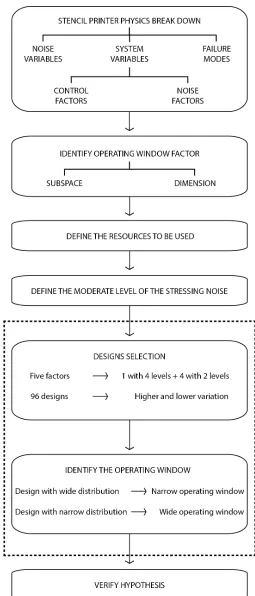
Methodology
The project will be developed based on the seven steps proposed by Clausing and Fey
(2004) to successfully apply the operating window concept. These steps consist of:
i) Identify the system critical functional variables through the analysis of the physics of the
system.
ii) Define the resources to be used on the development of robustness. The resources have to
represent the system and have to allow changes on the critical functional variables.
iii) Identify the failure modes to that affect the system and the noise variables excite the
failure modes and reduce the system performance;
iv) Summarize the identified system critical parameters and variables that affect this system;
v) Define the operating window of the selected factor by identifying the range that keeps the
failure modes constant;
vi) Adjust the system control variables to maximize the operating window range.
vii) Analyze the trade-off between time and level of robustness wanted in order to repeat the
cycle.
An adaptation of the steps will be used to fit the purpose of the research. In this study,
the operating window is not meant to be maximized, nor is a nominal set point to be defined. The
research aim, is simply to identify the operating window from a variety of possible design
configurations in order to prove the hypothesis that tight performance variations would lead to a
large operating window and vice versa. This will be necessary because of the resources
constraints that are present in the target application and the available stencils that had been
developed for a pervious experiment. In order to adapt the methodology proposed by Clausing
The methodology will start with an analysis of the system physics to identify the critical
parameters that compose this system. The operating widow factor and the noise factors to be
used will be identified based on the previous analysis. All the equipment, tools, and supplies
will be selected to represent the system functions. With all system factors identified, an
experiment will be carried out to test the performance of all available designs. Two designs with
opposed performance results will be selected and the operating window will be developed for
each one of them. Finally, an analysis of both operating window will be performed to identify
the predicted difference between these designs.
Materials
Stencil Printer.
Machine specification. A stencil printer is part of the surface mount technology (SMT)
necessary to manufacture printed circuit boards (PCB). Surface mount technology allows the
production of smaller, lighter, faster and cheaper PCBs. The stencil printer applies solder paste
to the PCB where the components will be placed (Omori & Miller, 1992). The solder paste is a
mixture of solder particles with flux. The solder particles are required to form solder joints while
the flux gives the flow characteristics of the paste and is the means by which the solder particles
are held together. A stencil is a metal plate with small holes (apertures) arranged in a pattern that
mirrors a specific layout for each PCB that will be processed through the stencil printer machine.
The apertures match each PCB spot (pads), where the solder paste will be applied. The solder
paste is spread over the stencil by a squeegee. The squeegee is a blade that runs over the stencil
during the printing process and pushes the solder paste into the stencil apertures (Prasad, 1997).
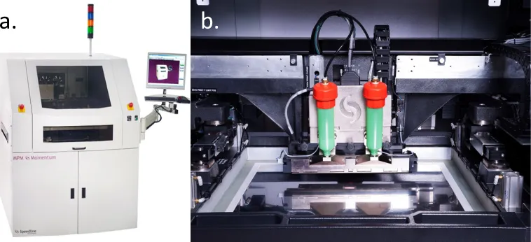
Figure 3 shows an image of the machine, the stencil and the squeegee blade as described. The
Figure 3. Stencil printer. This figure is a picture of the Stencil printer (a) and its parts (b).
Retrieved June 28, 2016
from http://www.speedlinetech.com. Copyright 2016 by the Illinois Tool Works.
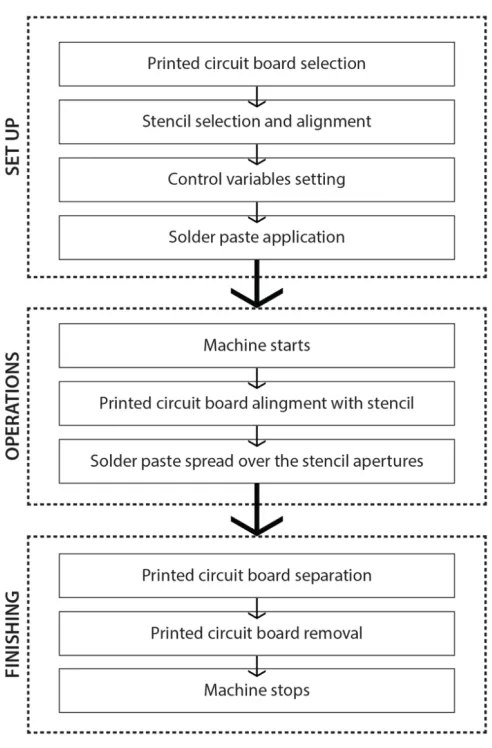
Operation. The process of applying a uniform quantity of solder paste to the PCB pads is
automatically done by the stencil printer after the control parameters are set. The setup involves
introducing and aligning the stencil that matches the PCB configuration, applying the variables’
set points on the machine computer and applying the proper quantity of solder paste over the
stencil. After the setup is done, the process starts and with the squeegee operation, the machine
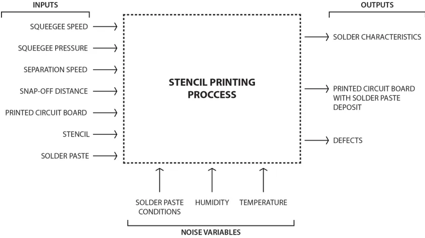
spread the solder paste that penetrates the apertures and settles on the PCB pads. Figure 4 shows
a detailed flowchart of the process. While the black box diagram in Figure 5 represents the
system inputs and outputs.
Figure 4. Stencil printer flowchart. This figure illustrated the steps of the stencil printer
production process.
A detailed printing process is shown in Figure 6. When the machine starts, the wafer
aligns with the stencil in a way that each pad match with the aperture on the stencil. After the
alignment, the wafer gets close to the stencil until the defined print gap. After the board is in
position, on step 1, the Squeegee starts rolling the solder paste. The apertures are filled with
solder paste that is pushed by the squeegee. On step 2, the board is detached from the stencil.
Figure 5. Stencil printer diagram. This figure illustrates the process inputs and outputs.
Motivation. The SMT assembly process is composed of Stencil printing, Component
placement, and Reflow soldering. Although the three processes have their own respective
operating difficulties, the solder paste printing process is responsible for 63.8% of the SMT
assembly defects (Mangin, 1991). In order to effectively reduce the defects on PCBs, the stencil
printing was selected. The design of a process that accounts for the failure modes and noise
effects is an alternative to minimize the defect rate of the SMT assembly instead of using the
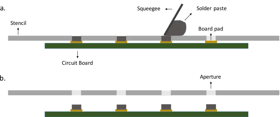
Figure 6. Solder paste printing process. This figure illustrates the detailed steps of the stencil
printing process, with the squeegee pushing the solder paste (a) and the stencil separation (b).
Failures. The failures will be identified by the application of a Fault Tree Analysis
(FTA). The FTA gives a visual representation of the failure events and their consequences,
making it easier to identify these failures and to mitigate them during the system design phase
(Shu, Cheng, & Chang, 2006).
Physics Breakdown. A deep understanding of the system physics has significant
importance to the application of the operating window methodology. To develop this
knowledge, the project starts by breaking down the system structure. The objective is to
understand the relationship between the system variables, failure modes, and noise variables.
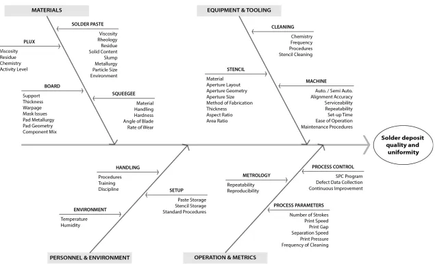
The system structure is shown in Figure 7. It can be seen that several factors can influence the
printing process. However, for the basis of this study, several of these factors will be kept
constant throughout the study.
Squeegee Solder paste
Circuit Board Stencil
Aperture Board pad
a.
Figure 7. Stencil printer variables. This figure illustrated the variables related to the stencil printer activity. Adapted from "Surface
Measurement. The system output will be considered the Transfer Efficiency (TE) of
solder paste from the stencils’ apertures. Amalu et al. (2011) states that the understanding of the
TE is vital for the stencil printing process. This measurement is a ratio of the volume of solder
paste deposited over the PCB to the aperture volume. Ideally this ratio should be 100%. A
100% Transfer Efficiency means that all solder paste that filled the aperture was transferred to
the PCB. Therefore, the apertures and solder paste volumes will be measured.
Aperture measurements. Aperture volumes are easily calculated from the stencil
manufacturing drawings. However, these values are nominal values and do not reflect the actual
values of each aperture as the manufacturing process is susceptible to variations. A good
practice is to design apertures on the corner of the stencil where it can be cut and measured with
precision. This would enable the use of aperture real dimensions and would enable a better
future replication. For the purpose of this project, this step will not be possible as the stencils
are already built and the data in the previous study is not available. However, an alternative will
be used. The actual aperture sizes from each stencil made with the Electroform and the Laser
technologies will be measured.
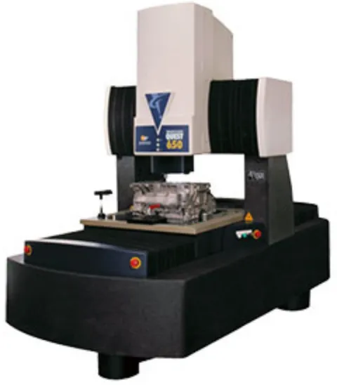
In order to measure the volume of each aperture, a SmartScope Quest 650 (shown in
Figure 8) from the Optical Gaging Products, Inc. (OGP) facility was used. The machine uses
optical sensors, a laser beam, and a touch probe to measure parts. The machine specifications
are shown in Appendix C. The machine is operated by Zone3 software. The software allows a
program to be written to measure parts features based on a computer-aided drafting (CAD)
model. In addition, the same program can be used to make measurements on other identical
parts. After the program is written all the measurements are made automatically on the CAD
Figure 8. SmartScope Quest 650. This figure illustrates the SmartScope Quest 650 machine.
Retrieved June 28, 2016 from
https://www.ogpnet.com/north-america/systems/video-multisensor/smartscope-quest/smartscope-quest-650/index. Copyright 2015 by Quality Vision
International, Inc.
Solder paste inspection. The solder paste deposit on the printed board was measured
using a Koh Young KY-3020T (see Figure 9). The machine is a bench-top metrology device and
its specifications are shown in Appendix D. The machine operates by emitting light from
different sources at predetermined angles onto a target. The lights generate a grid format and are
applied a predetermined number of times over a path. Pictures are obtained from this illuminated
path. The equipment is then able to measure the patterns on the images and calculate the target
Figure 9. Koh Young KY-3020T. This figure illustrates the Koh Young KY-3020T. Retrieved
June 28, 2016 from http://kohyoung.com/en/ky-3020t/. Copyright 2008 by Koh Young
Technology Inc.
To measure the solder deposit on the board, a drawing of the apertures is needed. The
machine generates the program based on the drawing and on the selected pads to be measured.
In order to reference the machine, the fiducials are used and several bare board are measured to
identify their pattern. With the program created the machine automatically measure the volume
of solder paste deposited on the PCB.
Operating Window Methodology
Identifying the operating window factor. The identification of the critical functional
variables is the first step in the development of robustness. To identify these variables it is
necessary to understand the system physics. With the understanding of the part interactions, it is
possible to identify the critical variables. This process is facilitated by the use of reliability tools
(Clausing & Fey, 2004).
Based on the previous step of the methodology an analysis of the system functions and
physics, it can be noted that several opposing failure modes are present. Failures can occur when
a small amount of solder paste is deposited on the pad. On the other hand, the excess of solder
paste can cause a different type of failure. These failures can be induced by variation in the
squeegee pressure and these failure boundaries can be defined by low and high pressure values,
respectively. At the lower level, the lack of pressure can result in not enough solder paste being
applied to the pad. On the other side, high-pressure levels can cause an increased amount of
solder paste to be deposited generating, for example, slumping, bridging, and scooping
phenomena. The squeegee pressure is considered as a strong operating window factor candidate
for this study.
Failure rate and noise level. Joseph and Wu (2004) identified that the main concept
behind the effectiveness of the Operating Window Methodology is the enlargement of the failure
probabilities. The method of failure excitation reduces the sample size necessary to estimate the
factors effects (Joseph & Wu, 2004) and it speeds up the learning cycles. As one of the
objectives during development is to identify when the system fails, the increased failure
frequency reduces the number of runs of the experimental strategy. Joseph and Wu (2004)
highlight the necessity to spend some effort to find a 50% failure probability known as the half
of the Lethal Dose (LD50). However, Clausing (2004) states that the exact percentage might not
be necessary, as long as the failure modes are significantly amplified. The LD50 value is also
questioned by Leitnaker and Mee (2004).
In this research the aim will be to amplify the failure rate but quantifying the failure rate
or getting to an exact fail rate number will not be a focus. In order to excite this failure
level. The objective is simply to reduce the number of samples necessary to find the operating
window.
Experimental plan
Before starting experiments, it is recommended to validate that the measuring system is
adequate as they have great impact on the identification of a product quality (Pan, 2006). This
will be done through a Gage Repeatability and Reproducibility (Gage R&R). This analysis will
identify if there is significant variability in the measuring system. Pan (2006), showed that the
level of variability due to the measurement system should be less than 10% specification width.
So, it will be possible to rely on the measurement system, if the variability due to Koh-Young
measurements is less than 10% of specification width.
The process of selecting two designs and identifying the operating window for both
require data collection. These data will be collected with two different experiments. First is
necessary to identify the distribution for each available design and to look at the effect of these
different design variables. This will be done through a full factorial design under normal
operating conditions. Secondly, in order to test the hypothesis of this thesis, the experiment is
performed to identify the operating window for two of the available designs. The OW will be
applied to the extreme cases to see if the variability and the operating window are indeed
correlated. This is done by a sequential trial and error approach under high fail rate operating
conditions.
Designs selection. The first experiment will serve as a pre-testing for the operating
window experimental strategy. It aims to identify designs with different distributions associated
with changes in the stencil design parameters. To assess a significant difference, the design with
experimental design is necessary to assess the distribution of each available design. As a
standard Robust Design approach, all the control parameters are fixed at a nominal value. All
the designs will be analyzed under the same printing conditions. This nominal level for each
control parameter is defined based on expertise and industry accepted standards. For each run, a
transfer efficiency distribution is plotted. The concept of the operation window is to be tested by
identifying the operating window for the factor’s levels from the two selected designs.
For the Stencil printer experimental design, five factors are to be evaluated as is shown
on Table 2. The apertures were manufactured with Laser, laser with nano-coat, electroformed
with nano-coat, and electroformed with nano-coat polished. For each stencil, there are also two
different thickness designs which are four and five mils. In addition, there are different aperture
designs for the type of component selected. It was selected the components with dimensions of
0.1”x0.05” (01005). The apertures for this component were manufactured in square, rounded
corner, and bow tie shapes. Moreover, there are apertures with different dimensions, 9x9 mils,
Table 2
Design factors and their levels.
Factors Manufacturing Stencil Type
Stencil
Thickness Aperture Design Aperture Size Orientation Aperture
Levels
Electroformed with
nano-coating 4 mils
Rounded
corners 9x9 mils Horizontal
Electroformed with
nano-coating polished
5 mils Sharp corners 10x8 mils Vertical
Laser Trapezoid
Laser with
nano-coating
Given the number of factors and their levels it would be needed 96 runs to assess all
factors combinations. For this reason, it would be reasonable to think in reducing the number of
runs, necessary to analyze all the factors, with a Taguchi Orthogonal array. However, to test the
hypothesis without any aliasing, we chose to run the full factorial design. Moreover, on a
product development effort, we want to test all the alternatives. Even though it could be possible
to reduce the number of runs, this is not a constraint for this experiment. In addition, because of
the board design, we will have four replicates at each run.
This experimental part of the present research is a replication of the study by Mohanty et
al. (2011). The same stencils and machinery were used. The only difference would be the use of
a different solder paste manufacturer. However, setting the stencil printer for the same
solder paste and an excess of solder paste was left over the stencil after the print (Figure 10).
This problem shows that the solder paste is not rolling smoothly and probably not filling the
apertures. The cause of this problem was assigned to the different solder paste used. Although
the same type was used, different properties can be found between manufacturers. The solder
paste property has a great impact on the printing quality (Prasad, 1997). The material viscosity
and its variations during the printing process are determinant factors for the entire SMT
mounting process. The incorrect storage and pre-production procedures can also change the
desired properties. The type of solder paste is based on the solder particles size. The types vary
from Type-1 to Type-6. The specification type for the PCB to be used is the Type-4 (Prasad,
1997).
Hence, the printing pressure was adjusted until a good flow of solder paste was found
(Figure 10). The pressure was changed from 16 to 22 pounds (lbs.). With these changes, the
standard setting to be used is as follow:
• Solder Paste – Loctite Type IV, lead-free paste
• Squeegee speed – 1 in. per second
• Squeegee pressure – 24 lbs.
• Separation distance – zero print gap
• Separation speed – 0.9843 in. per second
• Cleaning frequency – dry wipe after each print with vacuum suction
• Print direction – both rear-to-front and front-to-rear
• Number of prints – one replication after the third print
Figure 10. Printing flow. This figure illustrates a print where solder past stayed on the stencil
after the print (a) and a clean print (b).
The nominal design setting was based on the results of Mohanty et al. (2011). Their
results show that electroforming with nano-coating stencil has a greater process capability for all
the apertures. Mohanty et al. (2011) also conclude that the aperture Area Ratio (AR) is directly
correlated with the transfer efficiency increase and variance decrease. That being said, the
aperture with greater AR is a 9x9 mils aperture with rounded corners on a four mils thick stencil.
Moreover, they also conclude that there is no significant difference due to the apertures
orientation. The vertical orientation was selected as it presents a larger space between the
apertures during the print.
Constraints. Different noise factors affect the lower and upper thresholds. The lack of
solder deposited is hampered by solder paste with high particle size or a poor aperture finish.
One example is the finish allowed by the Laser technology compared to an Electroforming with
nano-coating polish. On the other side, a high stencil thickness or a high print gap should
generate a higher deposit of solder paste. But most of these factors are design parameters or
were already mitigated with the development of the stencil printing technology.
Squeegee Pressure = 16 lbs. Squeegee Pressure = 24 lbs.
In addition, physical design variables are harder to change and the operating window is
applied to its manufacturing process. On the stencil printer, the aperture sizes are one example.
The operating window methodology can be applied to the development of the stencil but its
application on the printing process will not enable changes to the apertures as the stencil is
already built. The manufacturing of a stencil is an expensive task and it is not readily available
for this research. For these reasons, the analysis of the aperture sizes is restricted to a set of
available stencils, selected to develop the experiment.
Identify the operating window. Experiments are developed to validate hypothesis and
theories about how a system works. They require the definition of the problem, the selection of
response, the identification of factors and factor levels, the design and execution of the
experiment, data analysis, and conclusions based on the analysis result (Montgomery, 2013).
The second experimental step will follow a trial and error approach. Although this
approach is criticized by many authors (Box, Hunter, & Hunter, 2005; Czitrom, 1999; Logothetis
& Wynn, 1994; Wu & Hamada, 2009), a sequential design will be used. It should be noted that
the trial and error method in the Operating Window methodology is not random. Rather it is
guided by the insights generated by failure. The trial and error sequence is similar to the one
used by Joseph and Wu (2002) to find the thresholds on their experiment. However, no
equations will be applied, instead, a more intuitive approach will be used. Sequential designs, in
comparison with a single experimental design, are preferred to identify how changes in the
design parameters affect the system performance in the design phase (Frey & Jugulum, 2006).
Some authors advocate the adaptation of experimental plan based on the data result (Daniel,
1973; Friedman & Savage, 1947; McDaniel & Ankenman, 2000; Qu & Wu, 2005). This allows
knowledge of the system, to identify key points of the system design. In the Operating Window
methodology this learning is speeded up by the high failure rated applied as the insights are
generated by the failures.
To define the system’s operating window, at the first time, it is necessary to set the
system to its best operating condition. On a development process, the setting would be defined
based on previous experience with a similar process. The second step is to input the fixed noise
variable and adjust the operating window variable to have a high failure rate. A stressing noise
level is set at a moderate level and its level is increased each time the operating window is
improved (Clausing, 2004).
For the upper threshold, Mohanty et al. (2011) applied a transfer efficiency limit of
140%. This was the value defined as a short circuit failure. Although for the lower limit,
Mohanty et al. (2011) applied a transfer efficiency limit of 60%, Anselm (personal
communication, June 3, 2016) claimed that in certain cases it is possible to have a good solder
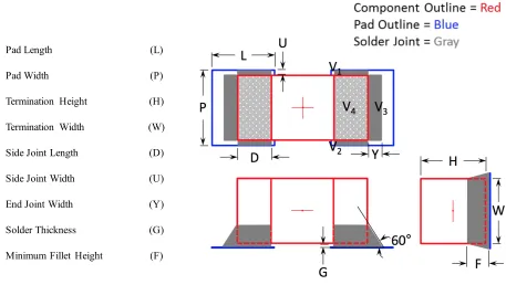
joint with transfer efficiency as low as 30%. A minimum print deposit was estimated for the
01005 components using the methodology applied by Schake and Whitmore (2016) for 008004
components. The minimum paste deposit is two times the minimum solder joint volume
(Equation 2) as the flux from the solder past occupy 50% (on average) of the total deposit
volume. The minimum joint volume is the sum of the solder joint volume from the sides of the
terminations (V1 and V2) (Equation 3), from the end of the termination (V3) (Equation 4) and
from the solder joint under the termination (V4) (Equation 5) as can be seen in Figure 11.
However, differently from what was used by Schake and Whitmore (2016), instead of just the
solder thickness (G) the joint volumes will be calculated using a triangle approximation as was