The Internal Validation of a National Model of Long Distance Traffic.

This is a repository copy of

The Internal Validation of a National Model of Long Distance

Traffic.

.

White Rose Research Online URL for this paper:

http://eprints.whiterose.ac.uk/2375/

Monograph:

Gunn, H.F., Kirby, H.R. and Murchland, J.D. (1982) The Internal Validation of a National

Model of Long Distance Traffic. Working Paper. Institute of Transport Studies, University of

Leeds , Leeds, UK.

Working Paper 164

[email protected] https://eprints.whiterose.ac.uk/ Reuse

Unless indicated otherwise, fulltext items are protected by copyright with all rights reserved. The copyright exception in section 29 of the Copyright, Designs and Patents Act 1988 allows the making of a single copy solely for the purpose of non-commercial research or private study within the limits of fair dealing. The publisher or other rights-holder may allow further reproduction and re-use of this version - refer to the White Rose Research Online record for this item. Where records identify the publisher as the copyright holder, users can verify any specific terms of use on the publisher’s website.

Takedown

If you consider content in White Rose Research Online to be in breach of UK law, please notify us by

White Rose Research Online

http://eprints.whiterose.ac.uk/

Institute of Transport Studies

University of Leeds

This is an ITS Working Paper produced and published by the University of

Leeds. ITS Working Papers are intended to provide information and encourage

discussion on a topic in advance of formal publication. They represent only the

views of the authors, and do not necessarily reflect the views or approval of the

sponsors.

White Rose Repository URL for this paper:

http://eprints.whiterose.ac.uk/

2375/

Published paper

Gunn, H.F., Kirby, H.R., Murchland, J.D. (1982)

The Internal Validation of a

National Model of Long Distance Traffic.

Institute of Transport Studies, University

of Leeds, Working Paper 164

.*king

Paper 164

THE ImTEFax vz4L,IDATIm OF

A

NATICNAL

O E L OF

IDXG

DISPANCE TRAFFIC

H.F.

Gunn, H.R. Kirby

and

J.D.

Wchland

Working Papers are intended t o provide information

and

encourage discussion on a topic i n advmzce of formal

publication.

They represent only the views o f the

authors and

do not necessarily r e f l e c t the view or

approval of the sponsors.

ABSTRACT

GUNN, H.F.,

H.R.

KIRBY and

J.D.

MURCHLAND (1982) The

internal validation of a national model of lona distance

traffic. Working Paper 164, Institute

-

for ?ransport

Studies, ~3iversity

of

Leeds, Leeds. (Unpublished.)

During 1980/81, the Department of Transport developed a

model for describing the distribution of private vehicle

trips between 642 districts in Great Britain, using data

from household and roadside interviews conducted in 1976

for the Regional Highways Traffic Model, and a new

formulation of the gravity model, called a composite

approach, in which shorter length movements were

described at a finer level of zonal detail than longer

movements. This report describes the results of an

independent validation exercise conducted for the

Department, in which the theoretical basis of the model

and its the quality of its fit to base year data were

examined. The report discusses model specification; input

data; calibration issues; and accuracy assessment. The

m a i n problems addressed included the treatment o f

intrazonal and terminal costs, which was thought to be

deficient; the trip-end estimates to which the model was

constrained, which were s h o w n to have substantial

variability and to be biassed (though the cause of the

latter could be readily removed), with some evidence of

geographical under-specification; and the differences

between roadside and household interview estimates. The

report includes a detailed examination of the composite

model specification and contains suggestions for

improving the way in which such models are fitted. The

main technical developments, for both theory and

practice, are the .methods developed for assessing the

accuracy of the fitted model and for examining the

quality of its fit with respect to the observed data,

taking account of the variances and covariances of

modelled and data values. Overall, the broad conclusion

was that, whilst there appeared to be broad compatibility

between modelled and onserved data in observed cells,

there w a s clear evidence o f inadequacy in certain

respects, such as for example underestimation o f

intradistr

ict trips.

This work was done in co-operation with Howard Humphreys

and Partners and Transportation Planning Associates, who

validated the model against independent external data;

their work is reported separately.

1. Summary and conclusions

1.1 Introduction 1.2 Main findings

Comments on model s p e c i f i c a t i o n Comments on input d a t a

Comments on c a l i b r a t i o n

Comments on accuracy assessment

1.3

Discussion 2. Model s p e c i f i c a t i o n

2.1 Composite matrices

2.2 Composite model 2.3 Composite c o s t s

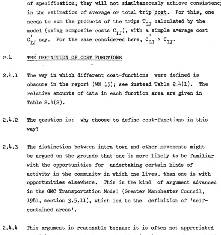
2.4 The d e f i n i t i o n of cost functions

2. $ I n t r a z o n a l model adjustments 3. Input data

3.1

I n t e r z o n a l c o s t s 3.2 Intrazonal c o s t s 3.3 Minor road t r a f f i c 3.4 Inactive households 3.5 Round t r i p s

3.6 Cordon-crossings comparison 3.7 Seasonal c o r r e c t i o n f a c t o r s

3.8

Merging of estimates 3.9 Trip end estimates

4.

Calibration

4.1

Xethod 4.2 P r i n c i p l e s 4.3 Uniqueness

4.4

Solution method

4.5 Calculat i o n a l economy 4.6 Convergence

4.7 Smoothing

PAGE

-

1

1

3 3

4

7

7

5.

Accuracy assessment

5.1

The components of model accuracy

5.2

On distinguishing model error and data error

5.3

The accuracy of observed

0-D

data

5.4

The accuracy of marginal totals

5.5

The accuracy of trip-end estimates

5.6

.The

accuracy of the fitted model's values

5.7

An overall view of model fit

5.8

The model fit in intra-district cells

5.9

The examination of residuals overall

6.

Acknowledgements

7.

References

8.

Appendix: Some descriptive statistics

8.1

Zone and cell statistics

8.2

Observed intradistrict trips

8.3

Modelled intradistrict trips

PAGE

-

55

56

58

59

60

61

65

67

70

72

Tables

Figures

. . . .

.

'A&i&es

:

.~t,pkifi~

'NO%&

'prddticed

i n

tkie

' ~ O W S C

'of

'*lie

'project

. . .

WN

51,.

Internal validation: some questions. KIRBY, H.R.

(1981, September

)

.

WN 2

Questions 'A'. KIRBY, H.R.

(1981,

September).

WN

3

The assessment of the likely accuracy of the National Model

on the basis of comparisons with calibration data sets.

GUNN,'

H.'F. '

(1981,.

September).

.

WN

4 '

Notes of a meeting at Leeds on 21 October.

1981.

KIRBY, H.R. (1981, October).

WN

5

The National Model Report: Initial reactions and requests for

further information.

_(1981,

November

)

.

WN

6

Approximating RDMVAR calculations. KIRBY, H.R

.

(1981,

November

)

.

I

7

Predict.ion error in fitted modcls.

FfUrlCJILAIJD, J.1).

(1981, November).

WN

8

Theoretical basis for multi-1evel.models. KIRBY,

H.R.

The National Cammercial Vehicle model: comments on c a l i b r a t i o n method. KIRBY, H.R. (1981, November).

The '3culo.h' matri:; n o b a s i s Tor conlpooitc modcl cxperimcntntion. GUiZ',

Il..

(1981, ~ e c e n b e r )

The Correspondence between Observed and Modelled Trip- Ends. ( r e g i o n a l zone]. GUNN, H.F. (1981, ~ e c e m b e r )

.

Approximate accuracy of r e g i o n a l zone s y n t h e t i c trip-ends.

Gum,

H.F. (1982, January).

~ ~ * r o x i m a t e accuracy of d i s t r i c t zone s y n t h e t i c trip-ends.

GUNN,. H.F. (1982, February).

I n t r a z o n a l and intra-town c o s t s . KIRBY, H.R. (1982, January).

Multiple d e t e r r e n c e f u n c t i o n s

-

d e f i n i t i o n s . KIRBY, H.R. (1982, February )

.

I n t r a z o n a l and intra-town c o s t s

-

f u r t h e r information. KIRBY,, H.R. (1982, February).

WN 1 7 Trips. KIRBY, H.R. @982, February).

WN 1 8 Simple versus c m p o s i t e treatment f o r a c e l l i n t h e National Model. MLIRCRLAND, J . D . (1982, February).

WN 1 9 How quasi-average c o s t s compare with simple average c o s t s f o r

a

s e l e c t i o n of d i s t r i c t p a i r s . KIRBY H.R. (1982, F e b r u a q ) . 20 Variance a d Covariance of t r i p c s t i m a t c s f r o n t h e splt5ct!.c

t r i p end mcthod of E i t t i n r : t h c firnvity modcl. ?7mCRL.AHCI, J.'l>.

(1982, ~ e . r c h ) .

lfii 21 Comparison of modcllcd

v&&s:

'irith independent d a t a MURCHLAND, J.D. (1982, 'March)

WN 22 Relationship between quasi-average and t r u e average c o s t s

f o r an exponential decay function. MURCHLAND, J.D. (1982, ~ a r c b ) .

WN 23 An examination of t h e r e s i d u a l s from t h e f i t t e d model

-

a l l purposes. GUNN, H.F. (1982, March).

WN 24 _{Cordon-crossings comparisons; t h e e f f e c t of s c a l i n g t h e d a t a .} MURCKLAND, J.D.

WN 25 Smoothing methods: some i s s u e s . (Correspondence, 1982)

WN 26 Observed and n a t i o n d model i n t r a d i s t r i c t t r i p s . MUXCRLAND, J . D . (1982. ~ ~ r i l ) .

LIST OF TABLES

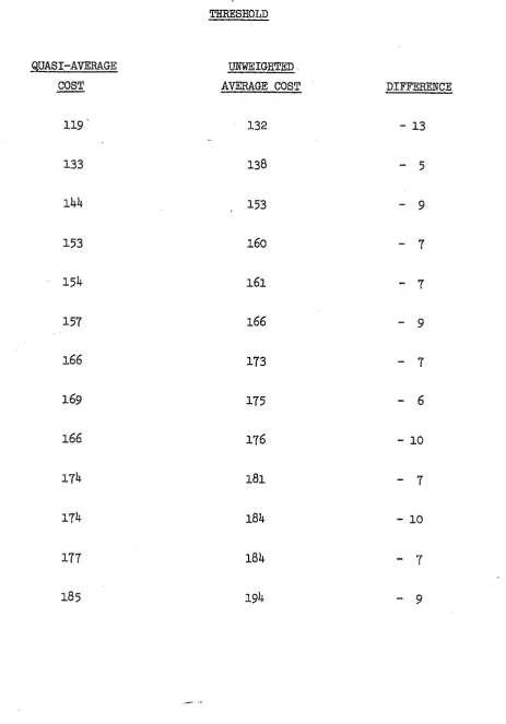
2.3(1)

Quasi-average and unweighted average costs near the

cost threshold.

2.3(2)

Proportional changes in cost function value for a

one-band shift in cost near the

100

pence threshold.

2.4(1)

The 'definition

of multiple deterrence functions.

2.4(2,)

The distribution of

HBW trips and travel amongst the

nine function areas.

3.3

Flows on interviewed, counted and uncounted roads by

cordon.

3.6

Cordon crossings

for the used and intended

data sets

3.9

Mean trip rates, observed and synthesised.

4.1

Size of the trip adjustment factor

5.4(1)

Row and column sums

,of

>observed

data and..their

accuracies

5.4(:2)

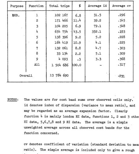
Cost band sums and accuracies.

5.5

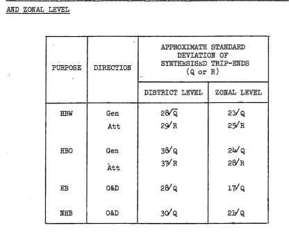
(1)

Approximate standard deviations in synthetic trip end

estimates at district and zonal level.

5.5(2)

Approximate

95

percent confidence intervals about the mean

numbers of trip-ends in a regional zone.

5.7

(1) Illustrative values for non-zero observed and modelled

values and their accuracies.

5.7(2)

Modelled estimates and their errors for observed cells

with zero observation

(HBW)

.

5.8

Districts with the worst-fitting intra-district estimates

(HBW).

.-. ..

PAGE

-

5.9(1) The mean r e s i d u a l and r e l a t i v e mean r e s i d u a l c a t e g o r i s e d by t r i p l e n g t h , and a r e a t y p e .

5.9(2)

The mean r e s i d u a l c a t e g o r i s e d by t r i p l e n g t h , a r e a t h e

'&d exp&sion f a c t o r .

5.9(3) Estimates of s t a n a a r d i s e d mean r e s i d u a l s i n each category of t r i p l e n g t h , a r e a t y p e and expansion f a c t o r .

5.9(4) Numbers. of observed c e l l s i n each category of t r i p l e n g t h ,

a r e a type and expansion f a c t o r .

5.9(5) Residual s t a t i s t i c s f o r t h e

6

c a t e g o r i e s w i t h l a r g e s t numbers o f c e l l s .

5.9('6) Residual s t a t i s t i c s f o r t h e 5 c a t e g o r i e s with l a r g e s t

numbers of t r i p s .

6.3

D i s t r i c t s with h i g h proportions of i n t r a d i s t r i c t movements.

PAGE

-

LIST OF FIGURES

Fig. 3.2(1)

Intrazonal time relationships used in the

National Model, and the previous RRPM Relationships.

Fig. 3.2(2)

Synthesised to observed intrazonal trips as a function

of zone size, for rural zone types. (Prior to

.

revision of intrazonal times.)

Fig. 3.2(3)

Synthesised to observed intrazonal trips as a function

of zone size, for urban zone types. (Prior to

revision of intrazonal times.

)

Fig.

5.5(1)

Synthesised versus observed

HBW

trip generations

(untransformed) (zonal level).

Fig. 5.5(2)

Synthesised versus observed HBW trip generations

(log-transformed) (zonal level).

Fig. 5.5(3)

Synthesised versus observed

HEW trip generations

(square root transformed) (zonal level).

Fig. 5.5(4)

Synthesised versus observed HBW trip generations

(square root transform) (district level).

PAGE

-

[image:10.595.67.567.111.786.2]

THE INTEEWAL VALIDATION OF A NATIONAL

MODE& OFLONG-DISTANCE TRAFFIC

1. SUMMARY AND CONCLUSIONS

1.1 INTRODUCTION

1.1.1 This r e p o r t summarises t h e work c a r r i e d out a t t h e I n s t i t u t e f o r

Transport Studies o f t h e University of Leeds t o a s s e s s t h e v a l i d i t y

of t h e Department of T r a n s p o r t ' s National Model

(NM)

of Long

Distance T r a f f i c . Because t h e commercial v e h i c l e model was not

ready f o r v a l i d a t i o n , t h e work was concerned almost e x c l u s i v e l y

with t h e p r i v a t e v e h i c l e model, a s described i n t h e first draft of Outram (1982).

The Leeds work was p r i m a r i l y concerned with t h e i n t e r n a l v a l i d a t i o n

of t h e model, t h a t i s , t h e performance of t h e model a s s t r u c t u r e d ,

and judged a g a i n s t t h e d a t a t o which it was f i t t e d . Judgements of model performance a g a i n s t independent d a t a s e t s ( i . e . ones

t o which t h e model was not f i t t e d ) , c o n s t i t u t e d t h e e x t e r n a l

v a l i d a t i o n , which was t h e r e s p o n s i b i l i t y of Howard Humphreys and

P a r t n e r s (HH&P), working with Transportation Planning Associates

(TPA). These consultants a l s o undertook those a s p e c t s o f t h e

i n t e r n a l v a l i d a t i o n which were most a p p r o p r i a t e l y handled by

t h e Department of T r a n s p o r t ' s ' v a l i d a t i o n and comparison' s u i t e

of computer programs, which t h e y had p r e v i o u s l y developed; t h e

Leeds team provided mathematical and s t a t i s t i c a l advice t o t h i s

work, with t h e l i n k s between t h e two geographically well-separated

teams being mainly maintained a s

a

r e s u l t of D r . Murchland being based i n London.

1.1.2 The i n t e r n a l v d i d a t i o n r e p o r t e d h e r e covers f o u r a s p e c t s ,

discussed i n succeeding s e c t i o n s of t h e r e p o r t , a s follows.

1.1.3

('a) Judgements on MODEL SPECIFICATION, including t h e d e f i n i t i o n of a composite matrix, composite model, composite c o s t s ,

m u l t i p l e d e t e r r e n c e f u n c t i o n s , and t h e e f f e c t s o f changes

i n i n t r a z o n a l cost s p e c i f i c a t i o n . a. .

1.1.4 _{( b ) Comments on INPUT} DATA and i t s adequacy, covering t h e i n t e r - zonal and i n t r a z o n a l cost d e f i n i t i o n s , t h e treatment o f minor road t r a f f i c , t h e correction f o r i n a c t i v e households,

s t a t i s t i c a l t e s t s f o r a cordon-crossings comparison of

household and roadside interview d a t a , t h e method of merging s e v e r a l t r i p estimates, and t h e trip-end estimates.

. . .

Section

3.

1.1.5 ( c ) Comments on t h e CALIBRATION method, including questions of p r i n c i p l e , uniqueness, s o l u t i o n method, c a l c u l a t i o n a l econow and t h e smoothing of t h e cost functions.

. . .

Section

4.

1.1.6

( 6 ) The making o f an ACCURACY ASSESSMENT of t h e f i t t e d model,

including showing how judgements about t h e extent of appreciable model mis-specification may b e made, t a k i n g

i n t o account t h e accuracies of t h e input d a t a ; t h e assessment of t h e accuracy of t h e trip-end estimates; t h e approximate a n a l y t i c formula f o r t h e accuracy of t h e f i t t e d model; t h e i n t e r p r e t a t i o n of t h e goodness of f i t of t h e model i n i n t r a d i s t r i c t c e l l s , and o v e r a l l .

. . .

Section 5.

1.1.7

The i n t e r n a l v a l i d a t i o n undertaken here

i s

complementary t o t h a t

undertaken by Howard Rumphreys and TPA, whose f i n a l r e p o r t should a l s o be r e f e r r e d t o . ( ~ o w a r d Humphreys and P a r t n e r s , 1982.)

1 . 1 . 8 I n t h e r e s t o f t h i s s e c t i o n we summarise t h e main findings of our stuqy, and consolidate t h e conslusions here r a t h e r than a t t h e end of t h e r e p o r t .

1.1.9

. An Appendix contains some s t a t i s t i c a l summaries of data t h a t a r e p e r t i n e n t t o our r e p o r t (see Section

8 ) .

1.1.10 For f u r t h e r t e c h n i c a l d e t a i l s , t h e reader i s r e f e r r e d t o t h e Working Notes ( W N ) produced o n . t h i s p r o j e c t . These a r e l i s t e d i n t h e

1 . 2

MAIN FINDINGS

Comments on model s p e c i f i c a t i o n

1 . 2 . 1 Given t h e choice of a g r a v i t y model t o describe t h e d i s t r i b u t i o n of t r i p s , and t h e existence of t h e RHTM d a t a base a t t h e 3613 regional zone l e v e l s of information, t h e procedures used t o determine t h e composite- approach and d e f i n e composite c o s t seem reasonable.' (2.1.1)

1.2.2 The composite model i t s e l f

mv

be described most simply a s a model a t t h e l e v e l of a 642 d i s t r i c t system*, which d i f f e r s from

conventional models only by having s e v e r a l c o s t values f o r nearby d i s t r i c t p a i r s i n s t e a d of t h e u s u a l one. (2.2.14)

The model has been s t r u c t u r e d i n such a way as t o enable

it

t o proxy t h e e f f e c t s of a model constructed a t t h e 3613 r e g i o n a l

zone l e v e l , but some of t h e assumptions used in s o doing have not been t e s t e d . (2.2.k)

1.2.3 The p r i v a t e v e h i c l e and commercial v e h i c l e models represent

d i f f e r e n t ways o f attempting t o achieve t h e same goal, o f

a

model f i t t e d at t h e 642 d i s t r i c t l e v e l being c o n s i s t e n t with t h a t which would have been obtained by aggregation of one f i t t e d at t h e 3613 zone l e v e l . We would expect t h e p r i v a t e v e h i c l e model t o give r a t h e r more r e f i n e d estimates of t h e c o s t f a c t o r s than t h e commercial v e h i c l e model but have no evidence f o r a s s e s s i n g how d i f f e r e n t t h e two approaches are. (2.3.11, 1 2 )

1.2.4 We have no d e f i n i t e evidence f o r b e l i e v i n g t h a t t h e r e i s any important b i a s introduced by t h e use of RHTM r a t h e r t h a n

NM

c o s t functions f o r d e f i n i n g composite c o s t s f o r remote d i s t r i c t p a i r s , b u t a number of p o s s i b l e problems have been i d e n t i f i e d , i n which perhaps t h e main one i s t h a t due t o using t h e RHTM HBW c o s t

..

'

Bate: However, a s 2 d i s t r i c t s had v i r t u a l l y no t r i p s it was v i r t u a l l y a

7 .

h c t i o n s t o define' composite cost f o r all t r i p purposes. (2.3.14 e t seq.)

1.2.5 The d e f i n i t i o n o f d i f f e r e n t deterrent functions f o r within-tom movements from those elsewhere may be argued on behavioural grounds (2.4.3) and t h e f u r t h e r d i s t i n c t i o n between r u r a l l u r b a n l metropolitan and London d i s t r i b u t i o n s was introduced t o r e f l e c t differences i n t h e s t r e n g t h of t h e public t r a n s p o r t a l t e r n a t i v e . We a r e however r a t h e r doubtful t h a t t h i s choice has been

s u b s t a n t i a t e d because t h e t e s t bed demonstration was pathological. (2.4.6) Guidelines on how b e s t t o define areas i n t h e matrix t o which d i f f e r e n t cost flmctions apply should b e developed

(2.4.10)

1.2.5 The adjustments made t o i n t r a z o n a l c o s t s , t o make them such a s t o make t h e model give b e t t e r agreement with observed i n t r a z o n a l t r i p s , complicates t h e model s p e c i f i c a t i o n , making

it

more d i f f i c u l t t o analyse t h e e r r o r p r o p e r t i e s i n t h e f i t t e d model,

'C&MmtB '-03 'tddut; 'data

1.2.7 The c a l c u l a t i o n o f 0-D generalised c o s t on t h e b a s i s of minimum time paths

i s

u n l i k e l y t o have an adverse influence on model f i t

(3.1.2). Any adverse e f f e c t s due t o t h e use of t h e same value of time f o r a l l t r i p purposes and regions, i r r e s p e c t i v e of r e g i o n a l v a r i a t i o n s i n income, w i l l be reduced a s a consequence of f i t t i n g multiple deterrence functions. ( 3 .l. 3 )

1.2.8 The reasons f o r t h e adjustments made t o i n t r a z o n a l c o s t s and t h e use of terminal cost corrections f o r movements between zones w i t B towis a r e oljscurely presented and t h e empirical evidence presented unconvincing. (3.2.3) However, t h e r e a r e sound

t h e o r e t i c a l reasons f o r making such changes (2.5.5

-

2.5.7; 3.1.5)

1.2.9 The b a s i s f o r a l l o c a t i n g purpose and t r i p l e n g t h c h a r a c t e r i s t i c s t o uninterviewed t r a f f i c on minor roads

i s

an improvement on t h e previous use of c o r r i d o r f a c t o r s (3.3.1

-

3.3.5) b u t , having been c a r r i e d out on a cordon-wide b a s i s , t h e r e may be d i r e c t i o n a l b i a s e s i n t h e

NM

observed flows which should be taken i n t o account when making comparisons with t h e f i t t e d model (whose parameters

should not be a f f e c t e d by t h e s e d i r e c t i o n a l b i a s e s ) o r with

independent d a t a (3.3.6

-

3.3.9). The assumed magnitude of flows onnon-countedroads should be substantiated. (3.3.4)

No comparisons were p o s s i b l e with t h e a l t e r n a t i v e more sophisticated c o r r i d o r expansion procedures developed by Martin and Voorhees

Associates (MVA), but

it

i s suggested t h a t t h e Department consider advising on t h e use of t h e MVA procedures i n any new 0-D t r a v e l surveys. (3.3.9

-

3.3.10)

1.2.10 The i n a c t i v e household c o r r e c t i o n f a c t o r , which was abandoned when providing trip-end estimates, was r e t a i n e d i n t h e observed d a t a s e t t o which t h e model was f i t t e d , and i s a major cause of discrepancies subsequently discovered. (3.4)

1.2.11 The i n v e s t i g a t i o n of round t r i p s c a r r i e d out i n t h e development of t h e National Model has p o t e n t i a l l y important implications f o r d a t a c o l l e c t i o n and model building s t r a t e g i e s , and deserves Rrrther i n v e s t i g a t i o n . The differences t h a t occur i n t h e

proportions and t r i p - l e n g t h s of single-leg t r i p s i n t h e outbound and inbound d i r e c t i o n s could have a s i g n i f i c a n t influence on t h e

R I t r i p l e n g t h c h a r a c t e r i s t i c s f o r a p a r t i c u l a r t r i p purpose even a t t h e n a t i o n a l l e v e l , s i n c e most roadside interviews were i n t h e outbound d i r e c t i o n . (3.5)

1.2.12 S t a t i s t i c a l comparisons of t h e household and roadside interview estimates of cordon crossing t r i p s d i d not r e v e a l a s i g n i f i c a n t difference between t h e d a t a s e t s f o r

HBW

and RBEB t r i p s ; but HBO

- 7 -

Comments on c a l i b r a t i o n

1.2.17 The p r i n c i p l e of f i t t i n g t h e model t o b e s t e s t i m a t e s of important

aggregate q u a n t i t i e s

-

h e r e , t r i p ends from t h e t r i p end model

and observed c o s t band sums

-

l a c k s t h e m e r i t s of a b e s t fit

method. Methods for t h e l a t t e r should continue t o b e developed. ( 4 . 2 )

1.2.18 Whilst

it

i s not known on t h e o r e t i c a l grounds whether t h e s o l u t i o n t o a. s y n t h e t i c trip-end model must be unique, empirical evidence, : g a i n e d from r e p e a t e d

runs

i n a demonstration d a t a s e t , have not

given evidence of non-uniqueness.

1.2.19 The composite model s t r u c t u r e could have been invoked more, t o

provide

a

more e f f i c i e n t c a l c u l a t i o n a l procedure.

(4.5)

1.2.20 E r r o r s due t o non-convergence t o t h e d e s i r e d row and column and

c o s t band c o n s t r a i n t s a r e n e g l i g i b l e compared t o t h e e r r o r s i n

t h e t r i p end e s t i m a t e s .

(4.6,3),

1.2.21 It i s not recommended t h a t t h e method of smoothing t h e c o s t

f u n c t i o n s i n t h e National Model be adopted f o r g e n e r a l use.

( 4 . 7 )

' " CdMeritg

' o ~

1.2.22) .The e r r o r i n t h e f i t t e d model value f o r a c e l l h a s two p a r t s : t h e

e r r o r a r i s i n g f r o m t h e u n c e r t a i n t y i n t h e d a t a t o which t h e model

i s f i t t e d , and inherent model b i a s ( 0 r ' m i s s p e c i f i c a t i o n e r r o r ' ) . The former i s c a l c u l a b l e ,

at

l e a s t approximately, from t h e known d a t a accuracy and t h e method of f i t t i n g . The b i a s , which i s t h e

e r r o r t h a t would s t i l l be present if t h e model were f i t t e d t o p e r f e c t l y accurate d a t a , i s harder t o get a t . Each r e s i d u a l i s an e s t i m a t e of

it. For most c e l l s t h e r e s i d u a l has a v e r y . l a r g e v a r i a n c e , because t h e observed value depends on such a

small

o r zero count. To a s s e s s b i a s e s f u r t h e r

it

seems necessary t o suppose a simple s t a t i s t i c a l d e s c r i p t i o n of them

-

i n p a r t i c u l a r , t h a t t h e y behave as i f t h e y were an independent random m u l t i p l i e r i n each c e l l

-

and attempt

t o f i t t h i s b i a s model, t a k i n g account of t h e d a t a and model

'

u n c e r t a i n t y .

1.2.23 The accuracy of t h e observed 0-D d a t a was c a l c u l a t e d i n d e t a i l

f o r each c e l l assuming t h a t t h e r e were no e r r o r s i n t h e v a r i o u s

expansion factors applied subsequently. (5.3) These were used

to provide accuracies for row, column and cost band sums. (5.4)

The coefficients of variation were about

3

percent for district

totals and (on average) 26 percent for cost band sums.

1.2.24

The inaccuracy of the synthetic trip end estimates (after

allowing for the bias between these and the observed row and

column sums) was found to be much better than was thought to be

the case towards the end of the

RIITM

project, but still substantial,

the coefficient of variation being of the order of

~ O O O / K

percent, where

Q

_{is the synthesised trip end value. (5.5)}

In practice this gives a range of coefficient of variation from

about 15 to about 50 percent.

(5.8.6)

1.2.25

The errors in district level trip ends are, surprisingly, greater

than those for zonal level trip ends, implying.that the trip end

models are underspecified, with some variable or variables

omitted which take similar values in nearby zones. This raises

doubts about the extrapolation of the trip end models to the

unobserved areas. (5.3.14

-

5.5.16)

1.2.26

An

approximate formula has been derived for the accuracy of a

gravity model fitted with the

NM

synthetic trip end technique.

(5.61

1.2.27 Modelled and observed values for a sample of observed cells (all

purposes combined) have been examined, together with their

accuracies, and the broad conclusion reached that, overal1,the

modelled values show a strong resemblance to the observed values,

with occasional big discrepancies. (5.7

)

1.2.28

Similar comparisons for intradistrid cells suggest that the

modelled values are lower than the observed values, %y about

7

1.2.29 The v a r i a t i o n i n t h e p a t t e r n of r e s i d u a l s over t h e matrix was examined by categorising them by t r i p l e n g t h , s i z e of expansion f a c t o r and by t y p e of movement (and by s i z e of modelled value, when appropriate). Neglecting v a r i a t i o n with expansion f a c t o r , t h e differences between modelled and observed values a r e more pronounced f o r t r i p s l e s s than 25 km, but were not judged t o b e important, t a k i n g i n t o account an approximate standard deviation of t h e r e s i d u a l . But t h e differences appear t o b e s t a t i s t i c a l l y s i g n i f i c a n t f o r all a r e a and t r i p l e n g t h c a t e g o r i e s with low

( < 1 0 ) expansion f a c t o r . Moreover, t h e r e a r e i n d i c a t i o n s t h a t , f o r t r i p s out of London-or between o t h e r Areas, t h e model i s performing d i f f e r e n t l y a s between c e l l s of low ( < 1 0 ) expansion f a c t o r (where t h e r e s i d u a l s a r e always n e g a t i v e ) and those of high (> 100) expansion f a c t o r , where t h e y a r e almost always p o s i t i v e . See s e c t i o n 1.3.3 f o r a comment on t h e a n a l y s i s and i t s implications. (See 5.9; t h e conclusions a r e more f u l l y described i n 5.9.22.

)

1.2.30 The simplest possible d e s c r i p t i o n s of t h e b i a s e s o r misspecification i n t h e d i s t r i b u t i o n model a r e t h a t t h e squared.biases a r e haphazard over t h e c e l l s of t h e matrix, with an average value which i s a constant, o r e l s e proportional t o t h e model value, o r t o i t s square. These t h r e e models of squared b i a s were f i t t e d t o t h e National Model. No s i g n i f i c a n t b i a s e s i n t h e s e simple o v e r a l l senses were found,

apparently because of t h e overwhelming number of c e l l s f o r which t h e r e s i d u a l was e i t h e r small o r very inaccurate.

1.3 'DISCUSSION

1.3.1 Clearly, t h e d a t a problems a f f e c t much o f t h e comparisons, r a t h e r than t h e model s p e c i f i c a t i o n . Much of t h i s can b e corrected e a s i l y

-

f o r example, t h e omission of t h e i n a c t i v e household correction f a c t o r from t h e 0-D d a t a , t h e r e v i s i o n of NHB t r i p end models t o exclude t r i p s by non-residents.

could, f o r example, be i n t r a z o n a l t r i p models o r ; more simply,

a model of long d i s t a n c e movements could be developed, i n which

t h e synthesised t r i p ends were t h o s e of longer d i s t a n c e

movements only.

1.3.3.

Concerning our assessment of t h e adequacy of t h e f i t t e d model, using t h e techniques described i n Sections

5.7

and 5.9, t h r e e p o i n t s may be made. The f i r s t p o i n t i s t h a t t h e techniques go w e l l beyond t h e c a p a b i l i t i e s of t h e Department's RDCOSM program,

i n s o f a r as ( i ) t h e y e&e account of v a r i a n c e s of b o t h model and d a t a , and t h e i r covariances; and (ii) t h e y allow p a t t e r n s i n t h e r e s i d u a l s t o be examined by segmenting t h e matrix according t o t h e

c h a r a c t e r i s t i c s of t h e o r i g i n - d e s t i n a t i o n p a i r s . Thus,

we

hope t h a t t h e Department

w i l l

consider providing enhanced software t o enable o t h e r p r a c t i t i o n e r s t o do t h e s e s o r t s of i n v e s t i g a t i o n s .

The second p o i n t i s t h a t t h e time s c a l e of t h e p r o j e c t d i d not

permit u s t o go a s f a r a s we should have l i k e d i n developing t h e s e

techniques. Having received t h e a p p r o p r i a t e d a t a with only about

t h r e e weeks t o go before t h e end of t h e c o n t r a c t , we were a b l e t o

i n v e s t i g a t e t h e r e s i d u a l s , t a k i n g account of t h e i r a c c u r a c i e s , f o r

o n l y a sample of c e l l s (Section 5.7) and a b l e t o i n v e s t i g a t e t h e

v a r i a t i o n s i n t h e r e s i d u a l s over a l l c e l l s , i n i t i a l l y only by

neglecting information on t h e i r a c c u r a c i e s (Section 5.9). The

t h i r d point a r i a e s from t h e second: because we were not a b l e i n

t h e time-scale t o i n t e g r a t e t h e s e two approaches t o examining

t h e r e s i d u a l s , nor t o c a r r y out f u r t h e r computer runs on t h e b a s i c

d a t a , we were f a c e d with some problems over i n t e r p r e t i n g t h e

evidence f r o m t h e s e two s e t s of analyses

.

I n i t i a l l y , t h e evidence from t h e two methods of examining t h e

r e s i d u a l s appeared t o c o n f l i c t , s o we s c r u t i n i s e d t h e a n a l y s i s more

fully subsequently, (including t a k i n g i n t o account a rough measure

of t h e accuracy of t h e r e s i d u a l s when examining t h e i r v a r i a t i o n

over a l l c e l l s . Our conclusions, summarised i n 1.2.29, and given

more f u l l y i n 5.9.22 mean t h a t though t h e evidence i s not a s

and high

(>loo)

expansion f a c t o r ( f o r t r i p s out of London o r

between o t h e r a r e a s ) , and t h i s gives r i s e t o t h e suspicion t h a t

t h i s

i s

i n p a r t a t t r i b u t a b l e t o d i f f e r e n c e s i n t h e H I and R I d a t a s e t s . To r e s o l v e t h i s adequately would r e q u i r e further d e t a i l e d

i n v e s t i g a t i o n o f t h e d a t a s e t s , and of t h e i r e r r o r s t r u c t u r e .

1.3.4. The main t h r u s t of our a n a l y s i s was d i r e c t e d

at

t h e e s t i m a t e s of t r i p s , not of t r a v e l . (= t r i p s

x

c o s t ) o r t r i p length. The f i n a l r e p o r t by HH&P, which includes analyses of observed and

modelled t r i p l e n g t h estimates, should be read i n conjunction

with t h i s r e p o r t f o r a f u l l a p p r e c i a t i o n of t h e National Model

c a l i b r a t i o n . (Howard Humphreys and P a r t n e r s , 1982)

1.3.5. Whilst t h e evidence f o r t h e accuracy o f t h e input d a t a and of

t h e f i t t e d model may appear alarming a t first s i g h t , t h i s may

be something one has t o g e t used t o i n t r a n s p o r t a t i o n modelling.

No s i m i l a r t r a n s p o r t a t i o n study i n t h i s country (and we suspect

anywhere e l s e i n t h e world) has been s u b j e c t t o such d e t a i l e d

s c r u t i n y a s has t h e National Model and i t s predecessor, t h e Regional Highways T r a f f i c Model. Transportation planning w i l l

have t o recognise t h a t t h e kinds and magnitudes of e r r o r s

presented i n t h i s r e p o r t a r e l i k e l y t o a r i s e i n very many

a p p l i c a t i o n s

-

and g r e a t e r a t t e n t i o n

w i l l

have t o be p a i d t o g e t t i n g clean d a t a and an appropriate model s p e c i f i c a t i o n .

2.0.1. The c h a r a c t e r i s t i c f e a t u r e of t h e composite approach t o d e s c r i b i n g

origin-destination movements

i s

t h a t s h o r t e r movements a r e t r e a t e d

at a f i n e r l e v e l of aggregation t h a n longer movements.

2.0.2. If t h e origin-destination d a t a

i s

s p e c i f i e d i n a composite way, a p o s s i b l e advantage over an e n t i r e l y f i n e - l e v e l s p e c i f i c a t i o n i s t h a t

small

amounts

of d a t a a r e grouped t o g e t h e r , thereby reducing t h e effects- of sampling v a r i a b i l i t y on t h e accuracy o f t h e parameter

estimates of a t r i p d i s t r i b u t i o n model.

2.0.3. If t h e t r i p d i s t r i b u t i o n model i s s p e c i f i e d i n a composite way, t h e main advantage i s a reduction i n computing c o s t s , compared with an e n t i r e l y fine-zone l e v e l of model s p e c i f i c a t i o n .

It i s not necessary t o specify both model and d a t a i n a composite

way. For example, Gunn (1977) showed how a conventional g r a v i t y model, s p e c i f i e d a t a f i n e zone l e v e l of d e t a i l , could be f i t t e d t o d a t a grouped i n a composite way.

2.0.4. The National Model s p e c i f i e s both d a t a and model i n a composite way. Since, i n t r a n s p o r t planning, t h i s i s pioneering new techniques, t h i s s e c t i o n seeks t o c l a r i f y t h e p r i n c i p l e s and procedures a s w e l l a s commenting upon t h e p a r t i c u l a r formulation adopted.

2.0.5. The d e f i n i t i o n s and s p e c i f i c a t i o n s o f , f o r example, composite matrices, a r e given i n Section 2.1; t h e model s p e c i f i c a t i o n i s given i n Section 2.2; and t h e cost s p e c i f i c a t i o n i s i n Section 2.3.

Note however t h a t both t h e cost and t h e model s p e c i f i c a t i o n have been adjusted i n t h e course o f t h e f i t t i n g procedure (discussed i n Section

41,

s o t h a t i n Sections 2.2 and 2.3 t h e r e i s some a n t i c i p a t i o n o f p o i n t s t h a t a r i s e l a t e r .

2.1.1 The various ways

in

which s h o r t e r movem~nts could be t r e a t e d

at

a f i n e r l e v e l of zonal aggregation t h a n longer movements were reviewed i n Kirby (1978). The method used i n t h e National Model i s probably t h e simplest and e a s i e s t t o implement. It has a two l e v e l hierarchy o f f i n e zones ( t h e so-called r e g i o n a l zones of

RHTM) and coarse zones ( c a l l e d d i s t r i c t s * ) i n which t r i p s a r e represented a s occurring a t e i t h e r t h e fine-zonelfine zone l e v e l o r coarse zone/coarse zone l e v e l . This avoids t h e f u r t h e r

complexity of representing coarse zonejfine zone i n t e r a c t i o n s e x p l i c i t l y .

/

2.1.2. Thus, i f I i s a d i s t r i c t of o r i g i n ( o r g e n e r a t i o n ) , and J i s a d i s t r i c t of d e s t i n a t i o n ( o r a t t r a c t i o n ) , and i f i?

j

a r e r e g i o n a l zones t h a t l i e r e s p e c t i v e l y i n I and J ( t h e shorthand

f o r which i s i E I , j E

J),

t h e multi-level system of zone-zone

movements may be presented roughly i n t h e following form

(supposing t h a t t h e nearby d i s t r i c t s have s i m i l a r numbers).

I7rorn

d i s t r i c t o r zone I

2.1.3. Some c e l l s of t h e d i s t r i c t - d i s t r i c t

-

(14) l e v e l o f i n t e r a c t i o n a r e subdivided i n t h e above t a b l e , i n t o what we c a l l sub-cells,

r e p r e s e n t i n g t h e zone-zone ( i - j ) l e v e l of i n t e r a c t i o n . A c e l l

t h a t i s not subdivided we s h a l l c a l l a simple c e l l ; a c e l l t h a t i s subdivided we s h a l l c a l l a com@oslte c e l l . An o r i g i n - d e s t i n a t i o n

matrix t h a t contains only simple c e l l s we c a l l a simple matrix:

one t h a t contains

a

mixture of simple and composite c e l l s we c a l l a ~omporiite

matrix.

For each of t h e c e l l s o r sub-cells t h e r e i s a

known journey c o s t . See t h e Appendix (Section

8)

f o r t h e numbers

of such c e l l s .

2.1.4. I n t h e National Model ( s e c t i o n 2.1) a d i s t r i c t t o d i s t r i c t (I-J)

p a i r was r e p r e s e n t e d a s a simple c e l l i f t h e c o s t of t r a v e l between

any r e g i o n a l zone p a i r included i n

it

exceeded a c e r t a i n t h r e s h o l d value. Thus, simple c e l l s connect remote d i s t r i c t p a i r s , composite

c e l l s connect nearby d i s t r i c t p a i r s . The d e c i s i o n on t h e c o s t

t h r e s h o l d

i s

a m a t t e r of judgement; t h e value o f 100 c o s t u n i t s (assuming an average speed of 60 km/h, t h i s corresponds t o a

d i s t a n c e of 37 km) was chosen on t h e grounds t h a t

it

reduced t h e t o t a l number of ( c e l l s and sub-cells) t o l e s s t h a n a m i l l i o n

(compared with t h e t h i r t e e n m i l l i o n i n t h e

RHTM simple matrix of

3613

x 3613 c e l l s ) . We do not know whether t h e fit of t h e model i s s e n s i t i v e t o t h e t h r e s h o l d value, but t h i n k it u n l i k e l y .

2.2. COMPOSITE 'MODEL

2.2.1. With observed zone-to-zone movements represented a t d i f f e r e n t l e v e l s

of s p a t i a l d e t a i l , t h e model s p e c i f i c a t i o n should i d e a l l y be such

t h a t e s t i m a t e s a t one l e v e l of d e t a i l a r e c o n s i s t e n t i n some sense

with those a t another. The key t o t h e t r a n s i t i o n i s having some information a v a i l a b l e a t t h e f i n e l e v e l of d e t a i l ; i n t h e case of

t h e National Model, both s y n t h e t i c trip-end e s t i m a t e s and zone-zone

c o s t s were a v a i l a b l e a t t h e f i n e l e v e l .

2.2.2. If

a

g r a v i t y model form i s required a t both f i n e and coarse l e v e l s of d e t a i l , t h e n t h e two forms m a y be represented as:

f o r c e l l s , i . e . remote d i s t r i c t s , and

t . .

=

a . bi

%

( c . .)

1 J 1

=

J

f o r sub-cells

,

i

.

e . r e g i o n a l zone-regional zone i n t e r a c t i o n s , i n nearby d i s t r i c t s , where:

ai, AI

=

generation f a c t o r s a t t h e f i n e and coarse l e v e l s

P

and f ( c . .)

,

'

F

(CIJ) 5 e f f e c t s of s u b k e l l c o s t s c i j , o r c e l l

13

c o s t s C on t h e i n t e r a c t i o n s between

IJ'

zone p a i r s i j o r d i s t r i c t p a i r s , IJ,

where t h e s u p e r s c r i p t P denotes t h e appropriate d e t e r r e n t function f o r t h a t p a r t of t h e matrix i n which IJ ( o r i j ) l i e s .

2.2.3 The consistency question

i s

one of r e l a t i n g ai t o AI, B. t o BJ, J

f P ( c .

. I

t o F ~ I C ~ ~ I .

1 J

For a f u l l y c o n s i s t e n t f i n e zone/coarse zone s p e c i f i c a t i o n of t r i p s , one would r e q u i r e t h a t :

I n t h e National Model, t h e first requirement t h a t t h i s l e d t o was t h a t t h e zonal parameters a t t h e f i n e zone l e v e l were r e l a t e d t o those a t t h e coarse l e v e l (which a r e t h e ones t o be estimated) by:

"i

=

-.

%

A, f o r i i n I (2:4)

Q1.

and

r b

=

j

-

B~ f o r j i n J (2:5)

R~

where qi, QI

=

t r i p generations synthesised i n f i n e zone i, coarse zone I , and a r e such t h a t C qi

=

i i n I Q~

r R

=

t r i p a t t r a c t i o n s synthesised i n f i n e zone

j,

coarse J - 0

zone J , and a r e such t h a t

C

r

=

RJ j i n J

j

2.2.4. Many o t h e r v a r i a n t s could have been taken. Whilst we have no evidence t o suggest t h a t t h e r e l a t i o n s h i p s (2:4; 2:5) a r e inadequate, we

should point out t h a t , so f a r a s we know, no-one has demonstrated t h a t , f o r a model f i t t e d t o f i n e zones, t h e parameters ( a i ) , ( b . )

.-. . J

ai/qi constant f o r nearby zones

and bj/rj

=

constant f o r nearby zones

The RHTM parameter estimates f o r t h e 3613 zone system could have been used t o demonstrate t h i s .

P

2.2.5. Any r e l a t i o n s h i p between F (CIJ) and f p ( c .

. I

may be e n t i r e l y

1 J

subsumed within t h e r e l a t i o n s h i p between coarse zone c o s t s CIJ

and f i n e zone c o s t s c . . ( f o r i j i n

IJ,

assuming only one cost

1 J

function i s included) by s e t t i n g :

f ( x ) = F(X) (2.6) ( s e e Note

*).

Further discussion of t h e cost r e l a t i o n s h i p s needed t o s a t i s f y (2.3) i s i n Section 2.3

2.2.6 I n f a c t , t h e r e l a t i o n s h i p (2.6) i s fundamental, r a t h e r than a supposition, s i n c e t h e d i s t r i c t - d i s t r i c t c o s t s were not a v a i l a b l e from a coarse zone network, but have had t o b e constructed from t h e zone t o zone c o s t s . T h i s i s discussed i n s e c t i o n 2.3.

2.2.7 If t h e r e i s no f u r t h e r requirement imposed t o meet t h e condition (2:3), then, f o r &'.*,array of c o s t s , t h e model may be

represented as:

f o r simple c e l l s

LM

( i . e . remote d i s t r i c t s )

_-

f o r s u b c e l l s i j 'witnfri ' a 60fipositt;e '6911

IJ

(This assumes t h e c o s t s C t o be given; a c t u a l l y t h e y a r e

LM

constructed, a s i n s e c t i o n 2.3)

2.2.8 The s u b s c r i p t s LM a r e introduced here t o r e i n f o r c e t h e d i s t i n c t i o n between simple and composite c e l l s , but l a t e r we use I3 throughout.

2.2.9 ' 'A 'simpler 'mat;lien@t:ical . . . ' I t ~ s c r i p t i 6 r i 'of 'We @avit:y 'model The

. , . . . . . . .

mathematical form of t h e model given i n Section 2.2 of t h e

NMLDTM

r e p o r t reduces t o t h e expressions i n (2:7) and (2:8). However, a s Murchland ( i n a note dated 24th Feb. 1981) and Gunn ( i n

WN

1 0 ) have pointed out, it i s p o s s i b l e t o express it even more simply. Before doing so however it i s b e s t t o express t h e separation function i n

(2:7,

8 )

i n a d i f f e r e n t way.

P

2.2.10. Since t h e separation function F

(C)

i s defined d i f f e r e n t l y i n d i f f e r e n t p a r t s o f t h e matrix but

i s

such t h a t , i n each p a r t , a parameter i s estimated f o r a given i n t e r v a l of c o s t , i n t e r v a l s k

can be defined corresonding t o both t h e c o s t - i n t e r v a l

-

function

P

d e f i n i t i o n such t h a t F (C)

=

F if c o s t C and p a r t P correspond K

2.2 .

I

1

For

'relbdte

'dlStrl6tS

'LM

where

=

1

if Cmlies in interval

K

=

0

otherwise.

and (2:8) becomes

:

2.2.12

'

'For

'SuW6lT$

'ij

'in

'fi@&?by

'd2Str2&%

'IJ

. . . , . . ~ . .

where d.

.

=

1

if c.

.

lies in the k"intemra1

I J ~ 1 J

=

0

otherwise.

2.2.13 The main simplification arises by adding the models estimates

for the composite cell as a whole.

Thus,

for (2:lO) for

'.rleBrby

'diStf%cts (cells

1

. .

which is the same form as (2:9),

but here

Obviously

0 <

DIJk

and

C

D

IJk

iI

1.

k

Note that since all the quantities on the right hand side of (2:12)

are dependent only on the trip-end estimates and costs, the value

Of

is known in advance of and is unaffected by the fitting

.-. ..

-

1 9

-

2.2.14 Summary : The model form may be most simply represented a s providing d i s t r i c t - d i s t r i c t estimal~es everywhere. These a l l have t h e form

For remote d i s t r i c t s t h e r e i s only one non-zero DIJk value. For nearby d i s t r i c t s t h e r e a r e s e v e r a l

DIJk

values (given by (2:12) ).

2.2.15 This r e p r e s e n t a t i o n of t h e model

w i l l

be used i n t h e r e s t of t h i s r e p o r t . I n both cases t h e summation n o t a t i o n

=

t

TIJk T ~ ~ +

a p p l i e s , although it must be remembered t h a t i f t h e c e l l IJ i s composite, t h e t r i p s

TIJ+

a r e associated with s e v e r a l c o s t bands.

2.2.16 Note t h a t , so far, t h e condition (2:3) f o r consistency i n t h e two l e v e l s of modelling

i s

not f u l l y met. The way i n which c o s t s were defined i n order t o achieve t h i s i n c e r t a i n r e s p e c t s

i s

discussed i n 2.3.

2.2.17 Note a l s o t h a t , f o r convenience, t h e functions w i l l be described a s having a categorised form

(F

r a t h e r than

'

F

( C . . ) ) throughout,

k 1 J

d e s p i t e t h e f a c t t h a t t h e functions were eventually smoothed. A s

already noted, t h e categorised notation conveniently i n d i c a t e s not only t h e c o s t value but a l s o t h e function type.

2.3 COMPOSITE 'COSTS

2.3.1. The National Model introduces a f u r t h e r r e l a t i o n s h i p between t h e

f i n e and coarse l e v e l s of modelling through t h e c o s t s c i j and

CIJ. This i s done i n two q u i t e d i s t i n c t ways.

2.3.2. (a]" 'For r e m o t e ' d i s t r l c t s , ' ' ' ' f o r both p r i v a t e and commercial

v e h i c l e models, t h e p r i n c i p l e i s e s s e n t i a l l y t h a t t h e c o s t s between remote d i s t r i c t s should be such t h a t t h e t r i p s given by

t h e coarse model would be equal t o t h a t given by a f i n e model (were

t h a t t o be applied t o such c e l l s ] .

That i s , i n a simple c e l l (LM), where (2:7) a p p l i e s , if (2:8) applied t h e r e t o o t h e n one would have

By t h e d e f i n i t i o n s i n s e c t i o n 2.4, one f u n c t i o n F a p p l i e s t o

all

p a i r s l m w i t h i n a given d i s t r i c t p a i r LM. Hence i s defined t h e doMpdgit6 d d s t f o r remote c e l l s :

(The term composite c o s t , and i t s d e f i n i t i o n , a r e equivalent t o t h o s e i n t h e modal s p l i t l i t e r a t u r e ) . The operation ( 2 ~ 1 4 ) i s

a l s o c a l l e d B quBsi--average.

2.3.3. The r i g h t hand s i d e of ( ~ 1 4 ) contains known q u a n t i t i e s , but a l s o

t h e Punction F(C], which

i s

t o be estimated. I n p r i n c i p l e , t h i s implies an i t e r a t i v e procedure. I n p r a c t i c e , t h e q u a n t i t i e s F(C)

were not t h o s e estimated i n t h e National Model c a l i b r a t i o n , b u t

t h o s e previously estimated i n t h e RFiTM c a l i b r a t i o n s , denoted by

Fo(C). say.

2.3.4. Whether t h e use of RHTM c o s t functions a s opposed t o National

Model c o s t f u n c t i o n s makes much d i f f e r e n c e i s discussed i n 2.3.14

e t seq. (The t h r e e RRI'M cost f u n c t i o n s f o r HBW were used t o

produce t h e composite c o s t s by [2:14), and t h e s e same c o s t s were

a l s o used f o r t h e o t h e r t h r e e purposes).

2.3.5. ( b ) For nearby d i s t r i c t s t h e p r i v a t e v e h i c l e and commercial

v e h i c l e models have taken d i f f e r e n t approaches s o f a r a s t h e use

of composite c o s t s a r e concerned.

2.3.6. I n t h e p r i v a t e v e h i c l e model, each nearby d i s t r i c t - d i s t r i c t p a i r

IJ i s t r e a t e d as a composite c e l l : t h e c o s t s between r e g i o n a l zone p a i r s i j w i t h i n IJ

ard

represented e x p l i c i t l y , a s shown i n Section 2.2.

2.3.7. I n t h e commercial v e h i c l e mode, nearby d i s t r i c t - d i s t r i c t p a i r s

IJ a r e t r e a t e d a s simple c e l l s , but w i t h a composite c o s t t h a t r e p r e s e n t s i m p l i c i t l y t h e s e v e r a l r e g i o n a l zone p a i r c o s t s w i t h i n

IJ. The composite c o s t i s defined a s

-

F-l

'IJ

-

Z.

-

qi

2

F ( c . . ) (2:16) i j i n

IJ

%

R~ 1 J

and, i n t h i s c a s e , t h e function 'F'

-

i s t h a t being f i t t e d t o t h e National Model, and t h u s CIJ i s updated a s p a r t of t h e i t e r a t i v e

procedure t h a t e s t i m a t e s (AI),

( B ~ )

and (Fk). I n c o n t r a s t t o t h e non-iterative use of t h e RHTM c o s t f u n c t i o n Fo(C) i n

c a l c u l a t i n g composite c o s t s f o r remote d i s t r i c t s , i t e r a t i v e

c a l c u l a t i o n s of composite cost f o r nearby d i s t r i c t s m a y be

a p p r o p r i a t e

.

2.3.8 The questions a r e , whether one method i s p r e f e r a b l e t o another; and would t h e y give very d i f f e r e n t r e s u l t s ?

the

AI,

B and F values) to a model of the private vehicle kind,

J

K

it is possible torepresent that solution in the form of a

model of the commercial vehicle kind, by appropriate choice of

composite costs for nearby districts. Thus there is an

equivalence between the two forms.

2.3.10 However, this does not mean to say that the

( A I ) ,

( B ~ )

and (FK)

values derived by fitting the model of the private vehicle kind

are the same as those derived by fitting the model of the commercial

vehicle kind. The former, as it represents fine zone-zone

movements explicitly, includes 0-D data at this finer level; the

latter includes

0-D

data only at the coarser level. For a given

observed district-district cell, the commercial vehicle model will

allocate all the trips to a single interval of trip cost (that

corresponding to the composite C

),

whereas the private vehicle

IJ

model will allocate the trips to several intervals of cost (those

corresponding to the ci

)

.

2.3.U

Hence one would expect the private vehicle model to give rather

more refined

(Fk) estimates than the commercial vehicle model,

essentially for costs below the

100

pence threshold, for the same

fitting method (i.e. synthetic trip end or partial matrix method).

2.3.12

There has however been no direct evaluation of the two model

forms, so there is no quantitative evidence for how different the

two approaches are.

2.3.13

(Note that the fitting methods used in the two cases were

different

-

that for the private vehicle model constrained the

model's row and column totals to synthesised trip-ends, that for

the commercial vehicle model did not. Since the private vehicle

model is the main concern of this study, there will be little

further discussion of the different approaches.

)

were used t o d e r i v e t h e c o s t s used f o r all f o u r purposes. The

RHTM f u n c t i o n s had been manually smoothed, and were monotonically

decreasing, s o t h a t t h e r e w a s no ambiguity a s t o what t h e i n v e r s e f u n c t i o n value was i n t a k i n g t h e quasi-average.

2.3.15 The question discussed i s , does

it

m a t t e r t h a t t h e o l d RHTM c o s t f u n c t i o n s ( o r r a t h e r , time functions a d j u s t e d t o a c o s t b a s i s )

were used i n (2:15) f o r remote c e l l s , a s opposed t o using c o s t

f u n c t i o n s obtained i n t h e National Model? The questions i s

p a r t i c u l a r l y a p p o s i t e f o r c e l l s near t h e 100 pence c o s t t h r e s h o l d ,

because, below t h i s t h r e s h o l d , t r i p s a r e estimated i n a way which

corresponds t o u s i n g t h e National Model f u n c t i o n t o define a

composite c o s t , a s i n 2:14 o r 2:16, and above it t o t h e use of RHTM f u n c t i o n v a l u e s , a s i n 2:15.

2.3.16 Although

we

have no evidence, t h i s ma~r not m a t t e r , d e s p i t e t h e f a c t t h a t t h e o l d f u n c t i o n s were obtained f o r

3

d i f f e r e n t ' a r e a s ' of t h e RBW matrix, as opposed t o

9

i n t h e National Model f o r each purpose ( s e e Section 2 . 4 ) . The reason i s t h a t t h e averaging represented by 2:15 i s being done f o r d i s t r i c t s t h a t a r e f a r a p a r t . A l l t h e c o s t s clm f o r remote d i s t r i c t s

LM

w i l l

(by

d e f i n i t i o n of t h e simple c e l l ) exceed t h e c o s t t h r e s h o l d of 100

pence. It seems u n l i k e l y t h a t t h e r e l a t i v e v a r i a t i o n of F(cl,)

over a l l t h e s u b c e l l s w i t h i n a given

LM w i l l make t h e quasi-

average given by (2:15) very d i f f e r e n t from a more s t r a i g h t f o r w a r d average c o s t ,

and

hence

it i s

u n l i k e l y t h a t i n a c c u r a c i e s i n t h e r e l a t i v e values of Fo

w i l l

have much e f f e c t on t h e quasi-average.

(By r e l a t i v e v a r i a t i o n , we mean t h a t due t o t h e s l o p e . )

2.3.17 Moreover, t h e main d i f f e r e n c e between t h e t h r e e f u n c t i o n t y p e s

used i n RHTM (urban, r u r a l , London) and t h e nine used i n t h e

National Model ( s e e S e c t i o n 2 . 4 ) , i s t h a t t h e l a t t e r distinguished

intra-town movements from t h e r e s t ; b u t t h e r e l a t i v e values f o r F(C) curves f o r t h e s e two types of movements f o r each o f t h e

National Model suburban/rural/metropolit an/London c a t e g o r i e s were broadly s i m i l a r .

2.3.18

The fact that the trip-ends used in forming the quasi-average

with the RHTM function (in 2:15) were not the same as those used

in fitting the National Model (and so appropriate to 2:16) is

likely. tohave only a negligible effect.

2.3.19

The main inconsistencies that are likely to arise are for journeys

other than home-based work. This is because only the

HBW RHTM

cost function was used to define composite costs for remote cells.

2.3.20 For a few cells, there may be inconsistencies due to the various

sub-cells within it having different

RHTM cost functions applied

to them (i.e., a mixture say of urban and rural). Note that the

situation does not arise with the National Model function, which

is of the same type for all sub-cells within a given district-

district cell.

2.3.21

Eknpirical evidence for the differences that are likely is

available from NATDEF output (reproduced in

WN

19).

This shows

that the quasi-averages given by (2:15) are almost always less

than the simple unweighted average cost. (Theory given in

WN

22 confirm that, for a convex cost function, the quasi-average

2:15 will always be less than the corresponding simple weighted

average. For a rapidly decreasing function, Fo, the quasi-average

will be close to the least of the costs in the sub-cells.) Most

of the quasi-averages are within 10 pence of the unweighted

average.

2.3.22

For the important region near the

100

pence threshold, Table

2.3(1) surnmarises some of the

WN

19

data. It is unlikely that

the use of National Model function values rather than RHTM function

would change the value of the quasi-average by as much as the

2.3.23 If one ignores t h e e f f e c t of any change t o t h e c a l i b r a t e d values

of t h e c o s t f u n c t i o n Fk, t h e n a change i n c o s t i n a p a r t i c u l a r

c e l l IJ t h a t implies a change from F t o F

+

aF i n t h e d e t e r r e n t

f u n c t i o n value

w i l l

generate a p r o p o r t i o n a l change i n t h e model's e s t i m a t e s of t r i p s i n t h a t c e l l given by, approximately,

where aIJ talres account of t h e row and column c o n s t r a i n t s , and

i s given approximately by

( ~ i r b ~ , 1973). I n many cases, a

w i l l

be n e g l i g i b l e near t h e IJ

100 pence t h r e s h o l d . The p r o p o r t i o n a l changes i n t h e numbers of

t r i p s f o r

a

one-band s h i f t i n c o s t a t t h e 100 pence t h r e s h o l d a r e given i n Table 2.3(2).

2.3.24 A s a general p o i n t , we n o t e t h a t , s i n c e t h e composite c o s t s f o r remote d i s t r i c t s a r e s o c l o s e t o t h e simple unweighted

average zone-zone c o s t s ( s e e

WN

l g ) , it seems p o s s i b l e t h a t a simple c o s t , from d i s t r i c t c e n t r o i d t o d i s t r i c t c e n t r o i d ,

mqr

have been adequate f o r t h e s e d i s t r i c t s . I n p r a c t i c e though,

s i n c e d i s t r i c t c e n t r o i d s were undefined and zone-zone c o s t s had

t o be used t o c a l c u l a t e an average c o s t between d i s t r i c t s , t h e r e

i s v i r t u e , and very l i t t l e e x t r a computational e f f o r t , i n c a l c u l a t i n g t h e composite c o s t s ( r a t h e r than s a y t h e average

c o s t ) f o r a l l d i s t r i c t p a i r s .

2.3.25 The main v i r t u e of c a l c u l a t i n g composite c o s t s f o r remote d i s t r i c t s

i s t h a t it reduces t h e r i s k of d i s c o n t i n u i t y a r i s i n g i n t h e treatment of c e l l s near t h e 100 pence t h r e s h o l d .

2.3.26 The c a l c u l a t i o n of average c o s t s It must be s t r e s s e d i n