Simulation Capabilities for Challenging Medical Imaging and Treatment Planning Problems

(1)

Simulation Capabilities for Challenging Medical Imaging and

Treatment Planning Problems

Thesis by

Catherine E. Beni

In Partial Fulfillment of the Requirements for the Degree of

Doctor of Philosophy

California Institute of Technology Pasadena, California

2011

(2)

c

2011

(3)

(4)

Acknowledgements

I owe my deepest gratitude to my advisor, Prof. Oscar P. Bruno. Working with him has been an honor and I have greatly benefited from his mentorship. This dissertation would not have been possible without his insight, guidance, contagious enthusiasm, and tremendous patience.

I would like to thank Sandia National Laboratories and the National Physical Sciences Consor-tium for encouraging me to begin my graduate studies and further enabling them by providing me with financial support.

It is a great pleasure for me to thank my friends and student colleagues at Caltech for all the care, laughter, and caffeine we shared over my years here. I am especially grateful to Greg Griffin, Andrew Kositsky, Nadine Dabby, Constantine Evans, Bao Ha, Alex Gittens, and Edwin Jimenez. My time here would not have been the same without them.

I greatly appreciate the care of all the administrative assistance at Caltech for helping the de-partments run smoothly and assisting me in many different ways. Sheila Shull, Syndey Garstang, and Tess Legaspi deserve special mention.

I am indebted to Riverside Community College, for taking a chance with such a young student and for all the wonderful mentoring and nurturing the faculty provided. I would especially like to thank Sal Rotella (for first letting me enroll at RCC), John “Biff” Pietro (for letting an eight year-old take his calculus class), Mary Legner, Rogelio Ruiz, and Sally Armstrong.

I wish to thank my undergraduate mentors at UCLA, for instilling a love of mathematics in me and for guiding me during my time there. For all their kind mentorship, I would like to thank in particular: Richard Elman (for convincing me to focus on applied mathematics), Chad Topaz (for introducing me to numerical analysis), Andrea Bertozzi, and John Garnett.

I would like to thank my sister, Juliet Beni, for standing by me, caring for me, and for patiently listening to more than her fair share of my long speeches about my thesis work.

(5)

(6)

Abstract

(7)

List of Figures

2.1 Illustration of a periodic extension off(x) = exp(sin(5.4πx−2.7π)−cos(2πx))

com-puted using the accelerated FC(Gram) method. . . 11

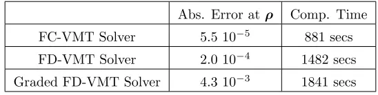
3.1 VMT geometry, as depicted in [42]. . . 23

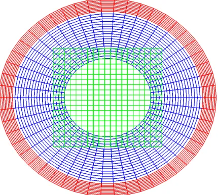
3.2 Meshing of the domain of solution Ω of the PDE (3.1). . . 25

3.3 Grids used by the Graded and Standard VMT solvers. . . 26

3.4 Solution of the steady state concentrationC(x, y) obtained through use of the FC-VMT solver for a VMT model with for three parameter sets . . . 34

4.1 Geometry corresponding to the control setup. . . 39

4.2 Grids used by the Explicit-Implict FC solver. . . 41

4.3 Numerical solution of the ad hoc control scheme (4.3) using the parameter choices D= 0.001,k= 10. . . 49

4.4 Numerical solution of the ad hoc control scheme (4.3) using the parameter choices D= 0.001,k= 20. . . 50

5.1 Variables and geometry associated with the Radon Transform. . . 53

5.2 The original 500×500 pixel Shepp-Logan phantom, and noiseless-data reconstruction resulting from the averaged mFBP and averaged Fej´er-mFBP algorithms. . . 61

5.3 MATLAB’s ‘iradon’ reconstructions of the 500×500 pixel Shepp-Logan phantom for noiseless data. . . 62

5.4 The original 500×500 pixel Shepp-Logan phantom and its Fej´er-mFBP reconstructions in the presence of 10.52% noise. . . 62

5.5 mFBP reconstructions of the 500×500 pixel Shepp-Logan phantom for noiseless data. 63 5.6 Fej´er-mFBP reconstructions of the 500×500 pixel Shepp-Logan phantom for noiseless data. . . 63

(10)

5.8 Shepp-Logan-mFBP and Fej´er-mFBP vs. Shepp-Logan-filtered FBP for the 500×500 pixel Shepp-Logan phantom with 18.38% noise. . . 66

B.1 The true values (solid lines) of CT(ρ, k) for k = 1, 2, 3 and 4 (Figures (i)–(iv)) and

ST(ρ, k) for k = 1, 2, 3 and 4 (Figures (v)–(viii)) plotted with their corresponding

(11)

List of Tables

3.1 Table of coefficients and coordinates used in each layer, including both the standard equispaced and expontially graded meshes in the vessel. The far left column provides the corresponding notation used in Section 2.3 for the description of the ADI algorithm. 27 3.2 Computational times required to obtain various accuracies for the parameter setDv₌

10−5_{, M}v _{= 10}−4 _{through use of each of the three VMT solvers. The solutions were}

computed over grids of sizeNx×Ny with the parameter choices Λ = 25, σf = 10−5,

andσs= 10−5. The entry marked by∗ was obtained using the selectionσf = 10−6. . 33

3.3 Computational times and errors at the critical midpointρ= ((xr−xl)/2, Ivm) using

Dv= 10−5, Mv= 10−4for the three VMT solvers. The solutions were computed over a 400×400 grid with the parameter choices Λ = 25,σf= 10−5, andσs= 10−5. . . . 35

(12)

Chapter 1

Introduction

Recent advances in medical science have given rise to many challenging computational problems. In some cases the resulting computational demands are so taxing that they simply overwhelm the capabilities of standard numerical methods. In this thesis we introduce three innovative numerical algorithms which, relying on novel spectral approaches, efficient time-stepping and domain meshing techniques for solution of Partial Differential Equations (PDEs) (enabling, in particular, effective resolution of extremely steep boundary layers in short computing times), improve significantly on existing numerical tools and provide, in fact, solutions to previously intractable medically-relevant problems. These methods were devoloped for use in two specific medical applications: 1) the field of therapeutic magnetic drug delivery, which involves the transport of magnetized particles through a convecting blood vessel and subsequent diffusion into surrounding tissues, and 2) the reconstruction of images obtained from Positron Emission Tomography (PET) scans.

1.1 Magnetic Drug Delivery

(13)

1.1.1 A Vessel-Membrane-Tissue Model

Several factors are most critical for understanding the efficacy of magnetically controlled drug tar-geting: 1) the geometry of the vasculature and velocity of the blood flow near the disease site, 2) the susceptibility of the magnetic particles (or ferrofluid) to the externally-applied magnetic forces, and 3) the in vivo diffusion of the particles into surrounding tissues. Past animal experi-ments [37, 38, 3, 53, 41] and phase I human clinical trials [38, 39, 35] have observed the accumulation of magnetic nanoparticles (or ferrofluid) by visual inspection, magnetic resonance imaging (MRI), and histology studies. These studies have shown that magnetic forces can concentrate micro and nanoparticles in vivo near the location of the external magnets. However, the details of the accumu-lation are not visible experimentally: the resolution in both MRI and visual inspection is not high enough to determine where magnetic forces have overcome blood velocity in the blood vessels and, because they must be carried out after the animal has been sacrificed and blood flow stopped, only partial knowledge of the particle behavior is provided through histology studies. Exact determina-tion of the locadetermina-tion of the ferrofluid accumuladetermina-tion via these methods is nearly impossible. In the recent publication [42], we proposed the use of numerical simulation of a simplified vessel geometry to better understand the accumulation behavior and evaluate the effects of external magnetic forces on the convection and diffusion of magnetic particles through the bloodstream and in membranes and tissues. While taking into account that the simulations are performed in an idealized geometry, the use of numerical simulation enables preliminary analysis and characterization of the particle behavior under different levels of diffusive and advective forces produced by the blood velocity and magnetic fields to be carried out both systematically and inexpensively. Such an analysis will thus, in turn, better enable the design of a method leading to confinement of the magnetically responsive particles to a particular region of the body.

An effective mathematical model of a blood vessel has been proposed by Grief and Richardson [26] and was extensively analyzed in [42] utilizing solver codes based on the numerical methods described in Chapter 3. The idealized geometry of the Grief and Richardson model is a version of the Krogh tissue cylinder [23] consisting of a lateral cross section of a blood vessel, including the endothelial layer (or membrane) and some surrounding tissue, with an external magnet situated below (see Figure 3.1). The characterizing equation of the resulting Vessel-Membrane-Tissue (VMT) geometry is given by the hyperbolic convection-diffusion PDE,

∂

∂tC(~r, t) =−∇ ·

h

C(~r, t)V~blood(~r, t)−D(~r)∇C(~r, t) +k(~r)C(~r, t)∇

|H(~~ r, t)|2i_, _(1.1)

with diffusion coefficient and advective terms varying over each layer.

(14)

figures prominently the strong concentration build-up, orboundary layer, that appears at the vessel-membrane interface: due to the discontinuity in diffusion coefficients over each layer, sharp boundary layers occur when the magnetic forces acting on the particles are strong enough to overcome the blood velocity, an effect that is particularly noticeable for the extremely small nondimensional diffusion coefficients present in realistic models of capillaries. Additionally, the advective forces provided by the blood velocity are significantly more powerful than the diffusive forces, thus giving rise to greatly disparate time scales; the development of an efficient time evolution methodology was necessary to produce steady state solutions in a reasonable amount of time.

In analyses prior to the work [42], numerical solution of the VMT problem was performed through use of the finite-element-based commercial software COMSOL Multiphysics (www.comsol.com). While capable of solving the VMT problem for large diffusion coefficients, the COMSOL software encountered many difficulties for the small diffusion coefficients inherent in realistic instances of the VMT model, especially for larger values of the magnetization. For example, some relevant drug absorption studies required solutions of convection-diffusion problems with (dimensionless) diffusion constants of the order of 10−7_{. In the preliminary studies performed on the COMSOL software,}

taking the diffusion and magnetization coefficients to equal 10−4 and 10−3 respectively, a steady state solution was reached in 36 hours of run time on a 3.16 GHz single processor of a quad-core Intel Xeon CPR X5460 computer with 32 GB of memory; the corresponding memory requirements to obtain the steady state solution for values of the diffusion and magnetization equal to 10−5

ex-ceeded the amount available on the same computer. Therefore, the medically relevant VMT model with diffusion constant equal to 10−7 _{and magnetization on the order of 10}−6 _{lies far outside the}

domain of applicability of the COMSOL software in the said computer. In contrast, the algorithms described in Chapter 3 produced accurate solutions for cases relevant to the contribution [42] with-out difficulty. For example, on a computer with a 2.66 GHz Intel Core 2 Duo processor and 4GB of memory, our solvers provide the required numerical solutions to the 10−4 _{and 10}−5 _{problems in}

under five minutes using 3 MB (not GB!) of memory and under fourteen minutes using 15 MB of memory, respectively. One of the most challenging cases considered in [42], in turn, for which the diffusion constant equals 10−7—a case that is very far from feasible for other methods—completed, using 25 MB of memory, in a six hour run.

1.1.2 Magnetically Enhanced Diffusion

(15)

interior of a domain—only unstable equillibria for ferrofluid particles may be attained with a static magnetic field. Several methods to bypass Earnshaw’s theorem have been proposed, including the implantation of magnetic materials, such as stents or wires, inside the body in order to create a local magnetic field [28, 49, 50], and the use of carefully placed external magnets so as to trap the ferrofluid against certain blood vessel walls [38, 39]. However, these techniques are not always viable solutions: surgical implantation of such objects in a patient may be undesirable or not feasible in a clinical setting and, due to the complex nature of the human blood vasculature network, entrapment of the particles against particular blood vessel walls has proven to be nearly impossible.

To overcome these limitations, Shapiro [51] proposed the development of a dynamic feedback-control scheme, where manipulation of the magnetically responsive particles is sought through dy-namic adjustment of the magnetic fields. (An example of the use of dydy-namic control to bypass Earnshaw’s theorem has been shown by the work of Potts et al. [47], wherein dynamic manipulation of a single electromagnet was used to suspend a drop of ferrofluid a distance away from the magnet.) Development of such a feedback-control scheme depends on evaluation of the effects of external magnetic forces on the convection and diffusion of magnetically responsive particles through the relevant tissues. In order to simplify the complex nature of these effects in standard vasculature geometries, and thus better understand the feasibility of such a control scheme, Shapiro [51] consid-ered the Grief and Richardson convection diffusion PDE (1.1) over an idealized domain: a circular region surrounded by eight electromagnets placed equally in a ring (see Figure 4.1). A zero-flux con-dition is imposed at the boundary of the domain in order to ensure no ferrofluid leaves the domain. Clearly, the design of adequate control schemes requires efficient numerical solution of such PDEs. This modification of the Grief and Richardson model may thus be utilized as a test bed for the development of numerical algorithms capable of evaluating such solutions accurately and efficiently. For the parameter values inherent in the medical configurations under consideration, the nu-merical PDE problems have proven quite challenging. For the small diffusion coefficients typically required to portray a relevant control setup, the imposition of the zero-flux boundary condition com-bined with the strong convective forces generated by the external magnetic field will cause extremely sharp boundary layers to rapidly appear near the boundary of the domain.

Once again, numerical studies presented in reference [51] were conducted using the commercial software package COMSOL Multiphysics. Similarly to the problems encountered for the VMT configuration, the COMSOL software was incapable of accurately resolving the steep boundary layer occurring for smaller values of diffusion coefficient. For example, numerical solution for the choice of diffusion coefficientD= 0.001 and magnetic driftk(~r) = 1 using the previously mentioned Intel Xeon CPR X5460 computer with 32 GB of memory was not feasible with the COMSOL software: to do so would require memory allocation greater than the computer’s capacity.

(16)

re-spectively, numerical solution of the ad hoc control scheme proposed in [51] was achieved with a maximum relative error of 10−2 _{in under two hours with 50 MB of memory by using the solvers}

introduced in Chapter 4 of this thesis.

1.2 FC-AD Methodology

The central challenge posed by both of these magnetic drug delivery simulations is the need for accurate and efficient resolution of boundary layers. Accurate resolution of steep boundary layers presents many difficulties for numerical solvers, at the heart of which is the requirement of a very fine spatial step size. This requirement imposes limitations on the type of numerical method efficiently useable: due to the requirement of such a fine mesh, explicit methods are rendered highly inefficient by the restrictive CFL condition ∆t∼O(∆x2_{) imposed on the time step.}

Further, because numerical solution over a nonrectangular domain is required for the idealized control setup described above and certainly necessary for more complicated models of the vasculature system, a standard finite differences approach over a Cartesian grid is not an efficient method of solution: such a scheme would require either a “staircasing” of the boundary of the domain or challenging, essentially impractical domain mapping strategies. Use of the first, rather simple technique reduces the spatial accuracy of the resulting finite difference method to first order. In addition, due to the absence of solution values outside the computational domain, finite difference stencils are forced to be made increasingly one-sided as the domain boundaries are approached. In general, stability is not achieved by simply using high-order centered difference methods in the interior of the domain and equally high-order biased stencils near the boundary. While there are several techniques to resolve this problem (such as the use of compact schemes [4] or Summation By Parts operators [40, 48]), these approaches are computationally expensive and must sacrifice some accuracy near the boundary to gain stability. Importantly, further, the multidomain strategies asociated with these algorithms require the discretizations of neighboring domains to match perfectly at common boundaries; see, e.g., [2] for details.

Numerical solution of PDEs over nonrectangular domains may also be produced by means of finite element and finite volume solvers. These algorithms do not provide an effective method of solution in the presence of boundary layers, however: because the spectral radii of differentiation operators based on nonuniformly spaced structured grids such as those used by finite element and finite volume methods will, in general, grow superlinearly, these techniques must also satisfy a stringent CFL condition for stability. High-order methods based on unstructured meshes give rise to similarly restrictive CFL constraints.

(17)

Implicit (ADI) methodology first introduced in 1955 by Peaceman and Rachford [45] in conjunction with the pseudospectral Fourier Continuation (FC) method, the resulting FC-AD algorithm can yield high-order accurate solutions with unconditional stability over general spatial domains at an essentially linear computational cost.

Many variants of the finite-difference-based ADI algorithm for the Heat and Laplace Equations have been put forward in the more than 50 years since its introduction, including methods for solution of various linear and nonlinear PDEs and solvers providing high-order spatial and temporal accuracy. Unconditionally stable alternating-direction methods preceding [16] could only achieve high-order accuracy for PDEs over domains representable as a union of a finite number of rectangular regions containing perfectly matched Cartesian discretizations. The few unconditionally stable high-order ADI algorithms that have been applied to nonrectangular geometries rely on use of domain mappings to transform the given problem into one posed over a rectangular geometry. Unfortunately, the inherently laborious construction of such domain mappings prohibits the use of these methods for most problems posed by engineering and scientific applications.

Alternating direction methodologies have also been previously used with spatial differentiation methods that do not depend on finite difference techniques. In particular, alternating direction approaches relying on a Fourier basis for differentiation have been proposed [5, 19, 43, 56]. However, despite efforts seeking to generalize these methods to more general domains, the application of previous Fourier-based techniques has also been restricted to rectangular geometries.

Because it is dependent on the Fourier approximation of nonperiodic functions, the use of Fourier bases in alternating directions methodologies requires resolution of a notoriuos problem in numerical analysis: the Gibbs phenomenon. A cornucopia of methods have been developed to resolve or reduce the detrimental effects of Gibbs phenomenon (see, e.g., [17, 25, 24, 12]). The Fourier Continuation method first proposed in [14, 13, 11] and accelerated in [16] eliminates the Gibbs phenomenon through the use of a “continuation” of the original function into a periodic extension; due to its periodic nature, the production of such a continuation enables the smooth approximation of the original function through use of Fourier series without difficulty. The use of this FC continuation strategy in conjunction with the alternating directions methodology, gives rise to the so-called FC-AD algorithm.

(18)

Addition-ally, the high-order accuracy and accurate handling of boundary condtitions offered by the FC-AD algorithm generally allow for accurate results with much coarser discretizations than otherwise nec-essary. These qualities make the FC-AD method a prime choice for the numerical solution of the convection-diffusion PDEs used to model magnetic drug delivery.

1.3 Positron Emission Tomography

Positron emission tomography (PET) is a nuclear imaging technique relying on the unique positron-emitting decay characteristics of radioactive tracer isotopes, or radiopharmeceuticals [20, 46]. After being introduced into the body (typically through intravenous injection) the radiopharmeceuticals undergo positron emission decay, ultimately leading to the emission of a pair of high-energy pho-tons traveling in approximately opposite directions. A ring of detectors placed around the body, the core component of the PET scanner, enables suitable detection of these high-energy photon pairs. Raw data collected from a PET scanner is simply a list of “coincidence events” representing near-simultaneous detection of the pair of high-energy photons by a pair of detectors. These coin-cident events, in turn, represent lines in space between the detector pairs along which the positron emission occured. The collection of coincidence events obtained from a PET scanner is described mathematically by the Radon transform [44, 7, 8, 6]; reconstruction of the desired image follows from appropriate inversion of the Radon transform.

(19)

1.4 Overview of Chapters

(20)

Chapter 2

Overview of FC Methodology

2.1 Fourier Continuation Basics

The Fourier Continuation (FC) methodology first introduced in [11, 13] and then accelerated in [16] is a central element in a class of unconditionally stable implicit PDE solvers, the FC-AD meth-ods, for linear constant [16] and variable-coefficient [15] PDEs in general domains. At the heart of this methodology is an accelerated periodic-continuation algorithm enabling a smooth Fourier rep-resentation of nonperiodic functions without the Gibbs ringing effect inherent in standard Fourier series approximations of nonperiodic functions. Indeed, by constructing a periodic continuation of the function in a domain significantly larger than the original interval, the resulting FC method smoothly resolves the detrimental oscillatory effects of Gibbs phenomenon. In this chapter, we pro-vide the basic outlines for implementation of two Fourier continuation methods: the unaccelerated FC(SVD) method presented in [13] and the accelerated FC(Gram) method first introduced in [16]. To facilitate explanation, we will consider both the FC algorithms over the unit interval [0,1]; ap-plication to a general interval easily follows from a simple scaling and translation of the discrete grid.

Consider a smooth functionf(x) for which the point valuesfj=f(xj) are given over the discrete

gridxj, j= 0, ..., N−1∈[0,1],

xj =j h, j = 0, ..., N−1, h= 1/(N−1).

For a given valueb >1, the Fourier continuation algorithm prescribes a method of construction of a b-periodic trigonometric polynomial,

fc(x) = X

k∈t(M)

ake

2πi

(21)

with

fc(xj) =f(xj) forj = 0, ..., N−1.

that approximatesf(x) in the interval [0,1]. The index functiont(M) is given by t(M) ={j∈N:

−M/2 + 1 ≤j ≤M/2} for M even and t(M) = {j ∈N: −(M −1)/2 ≤j ≤(M −1)/2} for M

odd. Selection of the bandwith M and the period b depends on the FC method used and will be determined in what follows. It is important to note that for b= 1, the continuationfc_{(x) reduces}

to the discrete Fourier transform off(x), and thus typically suffer from Gibbs phenomenon near the endpointsx= 0,1. Selecting b >1, on the other hand, allows forfc_{(x) to smoothly transition from}

the values off(x) nearx= 1 to the values off(x) nearx= 0 without oscillatory effects.

The basic, unaccelerated FC algorithm presented in [13] obtains the coefficients ak through

solution of the least-squares system

min

{ak:k∈t(M)}

N−1

X

j=0

X

k∈t(M)

ake

2πi

b kxj ₋_f_(x

j)

2

. (2.2)

Numerical results [13] have shown that it is advantageous to use a Singular Value Decomposition (SVD) to solve least-squares system (2.2); to better distinguish it from the accelerated FC algorithm presented below, we henceforth refer to this FC method as FC(SVD). Figure 2.1 presents a typical periodic continuation produced by application of the FC(SVD) method to function values off(x) = exp(sin(5.4πx−2.7π)−cos(2πx)) given in the interval [0,1].

While adequate for applications requring a small number of highly-accurate continuations, such as the high-order surface representations in [13], theO(N3_{) computational cost of one application of the}

FC(SVD) method is significantly higher than desirable for use in an algorithm dependent on the rapid computation of many periodic continuations, such as the FC-AD PDE solver introduced in [16, 15] and generalized in Section 2.3 of this text. Indeed, because both of these FC-based PDE solvers depend on computation ofO(N2) continuations per time-step, the high cost per continuation required by the FC(SVD) algorithm would render such solvers extremely infefficient. Recently, [16] overcame this issue by introducing a significantly accelerated FC method, the FC(Gram) algorithm. To highlight the differences between the FC(SVD) method and the accelerated FC algorithm presented in [16] and used in the numerical solvers introduced this text, a brief outline of the FC(Gram) method is provided in the remainder of this section.

As mentioned earlier in this section, a primary component of the general Fourier continuation method is the generation of a discrete periodic extension of the given function values into a longer interval [1, b]. Such an extension can be obtained by appending an additionalnd>0 function values

(22)

[image:22.612.116.548.77.235.2]

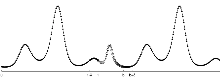
0 1-δ 1 b b+δ

Figure 2.1: Illustration of a periodic extension off(x) = exp(sin(5.4πx−2.7π)−cos(2πx)) computed using the accelerated FC(Gram) method, including the original function values (solid circles) and the extended function values (open circles). The thick black lines depict the function values over matching intervalsSleft andSright.

is produced, an application of the FFT algorithm to the newly extended discrete function values in the interval [0, b] yields the coefficientsakof the Fourier continuationfc(x) (as seen in equation (2.1));

the resulting approximation has bandwidthM =N+nd and periodb= (N+nd)/(N−1).

In the FC(Gram) algorithm, the main idea underlying the construction of thendextension values

mentioned above involves consideration of both the given function f defined in the interval [0,1] together with the translationf(x−b) defined in the interval [b,1 +b] (depicted as thin black lines with solid circles in Figure 2.1). Selecting a positive integer nδ, we define the “matching intervals”

Sright={xj|j=N−nδ, N−nδ+ 1, ..., N−1}to be the set ofnδ right-most discretization points in

the interval [0,1] andSleft ={b+xj|j= 0,1, ..., nδ−1} to be the set ofnδ left-most discretization

points in the interval [b,1 +b]. Loosely speaking, thend function values sought are obtained as the

point values of an auxiliary trigonometric polynomial produced by means of a least-squares fit to the function values off(x) overSright and the translationf(x−b) overSleft.

The construction of such a trigonometric polynomial proceeds by considering two orthonormal bases of Gram polynomials of degree< m. These bases, denoted by Pright and Pleft, are generated

through application of the Gram-Schmidt orthonormalization process with inner products

hg, hiright =

X

{xj∈Sright}

g(xj)h(xj), and

hg, hileft =

X

{xj∈Sleft}

g(xj−b)h(xj−b),

respectively, to the standard polynomial basis {1, x, x2_{, ..., x}m−1_}_{. As fully detailed in [16], the}

(23)

poly-nomial in Pright to a given polynomial in Pleft over the interval [1, b] by applying the FC(SVD)

algorithm to discrete data sets of the form{p(xj)|xj∈Sright} ∪ {q(xj)|xj ∈Sleft} for each

polyno-mialp∈Pright and q∈Pleft. This set of precomputed transition functions effectively forms a basis

of smooth transition functions from function values inSright to function values in Sleft. Thus, by

noticing that the given function values of f(x) in Sright and f(x−b) inSleft may be expressed as

linear combinations of the Gram polynomials in Pright andPleft respectively, it follows that we can

quickly compute a smooth transition from f(x) tof(x−b) in the interval [1, b] as an appropriate linear combination of the precomputed smooth transition functions.

An illustration of the full periodic-extension procedure is provided in Figure 2.1. As indicated in Figure 2.1, the nd extension values we seek are given simply as the values of this new smooth

transition function over the discrete grid 1 +xj, j = 0, ..., nd−1. An application of the discrete

Fourier transform in the interval [0, b] to the function values fj appended to the additional nd

extended function values yields the desired trigonometric continuation polynomialfc_(x).

Remark 2.1.1 Once a continuous continuation functionfc_{(x) has been obtained, numerical}

ap-proximations of the derivatives off(x) can easily be computed with spectral accuracy through direct differentiation offc(x):

df dx ≈

dfc dx =

X

k∈t(M)

2πiak

b e

2πi

b kx_. _(2.3)

The overall procedure for approximating one-dimensional derivatives of a given vector of function values,f(xj), j= 0, ..., N−1 thus consists of application of the FC method followed by an

applica-tion of the differential operator (2.3); clearly, derivatives of higher order can be produced similarly. Derivatives in multiple spatial dimensions on a structured mesh are implemented through successive line-by-line applications of the FC algorithm and differential operator in each coordinate direction. The behavior of the two-dimensional algorithm is straightforward, simply sweeping through hori-zontal and vertical lines of grid points and applying the one-dimensional differentiation algorithm in the corresponding coordinate; generalization to higher dimensions and higher-order derivatives is similarly straightforward.

2.2 Explicit Solver

Recalling the accurate FC-based method for the approximation of spatial derivatives presented in Remark 2.1.1 of Section 2.1, it is a straightforward matter to prescribe an explicit PDE solver: the algorithm proceeds, simply, by iterating a time-marching scheme. For the Explicit-Implicit and Implicit-Implicit FC solvers described in Chapter 4, we made use of the second-order Runge-Kutta time-marching scheme known as Heun’s method. In detail, denotingCn ₌_n∆t_and_Cn ₌_{C(u, v, t}n_),

(24)

second-order Runge-Kutta scheme,

˜

Cn+1=Cn+ ∆tL[Cn], Cn+1=Cn+∆t

2

L[Cn] +L[ ˜Cn+1],

(2.4)

with

L[C] =~κ(u, v)· ∇2_C₊_~_{λ(u, v)}_{· ∇}_C₊_ν_{(u, v)C}₊_{Q(u, v, t).}

The spatial derivatives present in application of the differential operatorLare approximated by the previously described FC method.

2.3 Alternating Directions Implicit

As mentioned in Section 2.2, an explicit method needs to satisfy the CFL condition 4t ∼F(4x) (specifically ∆t∼O(∆x2_{) for the problems under consideration in this thesis) to ensure numerical}

stability; the very fine discretization mesh required to resolve the boundary layers occurring in magnetic drug delivery problems therefore places a severe restriction on the maximum time step useable by an explicit method. In order to overcome this restriction, the solvers presented in this text make use of an efficient FC-AD implicit solver [16, 15]. Based on the Alternating Directions Implicit (ADI) method first developed by Peaceman and Rachford in 1955 [45], the FC-AD solver relies on line-by-line solution of ordinary differential equations (ODEs) that arise from factorization of the partial differential operator into differential operators of each variable; the resulting ODEs are then, in turn, solved for using an efficient FC method. In this section, a description of the FC-AD method for solution of a generalized version of the PDE (1.1) is provided. This generalization is chosen to allow for easy adaptation to the various convection-diffusion equations for the solution of each of the magnetic drug delivery problems presented in later chapters. An outline of the efficient FC-based ODE solvers used will be provided in Section 2.4.

Consider the general convection-diffusion PDE:

~

κ(u, v)· ∇2_C₊_~_{λ(u, v)}_{· ∇}_C₊_ν_{(u, v)C}₊_{Q(u, v, t) =}_C

t, (u, v, t)∈ Ω×(0, T],

a(u, v)C(u, v, t) +b(u, v) ∂C(u, v, t)

∂n =G(u, v, t), (u, v, t)∈∂Ω×(0, T], C(u, v,0) =C0(u, v), (u, v)∈Ω,

(2.5)

where Ω∈R2 is a smoothly bounded domain and~κ= (κu(u, v), κv(u, v)),~λ= (λu(u, v), λv(u, v)),

ν, Q, a, b, G, andC0 are all smooth functions. Lettingtn =n∆t, Cn = C(u, v, tn), and Qn+

1 2 =

(25)

difference scheme to obtain Cn+1−Cn

∆t =

1 2

~

κ· ∇2₊_~_λ_{· ∇}₊_ν_(Cn+1₊_Cn_{) +}_Qn+1

2 ₊_E₁_{(u, v,}_∆t),

where

E1(u, v,∆t)∼O(∆t2)

is the truncation error. Grouping together the terms forCn _and_Cn+1 _yields

1−∆t

2

~

κ· ∇2₊_~_λ_{· ∇}₊_ν

Cn+1=

1 +∆t 2

~

κ· ∇2+~λ· ∇+ν

Cn+ ∆tQn+12 _{+ ∆tE}₁_{(u, v, t),}

which can, in turn, be expressed in the form

1−∆t

2

κu ∂

2

∂u2+λ

u ∂

∂u+ν 1− ∆t

2

κv ∂

2

∂v2+λ

v ∂

∂v

Cn+1=

1 + ∆t 2

κu ∂

2

∂u2+λ

u ∂

∂u+ν 1 + ∆t

2

κv ∂

2

∂v2+λ

v ∂

∂v

Cn + ∆tQn+12 _{+ ∆tE}₁_{(u, v,}_{∆t) +}_E₂_{(u, v,}_∆t),

(2.6)

after appropriate factorization of the differential operators. A simple calculation shows that the truncation error E2(u, v,∆t) that arises from factoring the differential operators is on the order of

O(∆t2). For ease of explanation, we introduce the notation

Au=

κu ∂

2

∂u2 +λ

u ∂

∂u+ν

,

Av=

κv ∂

2

∂v2 +λ

v ∂

∂v

,

and rewrite (2.6) in the simpler form

1−∆t

2 Au 1− ∆t

2 Av

Cn+1=

1 +∆t

2 Au 1 + ∆t

2 Av

Cn +∆tQn+12 ₊O_(∆t2_).

(2.7)

Finally, making use of the approximation

Qn+12 =1

2

1 + ∆t 2 Au

_∆t

2 Q

n+1 4+1

2

1 +∆t 2 Au

_∆t

2 Q

n+3

4 +E₃(u, v, t) (2.8)

(26)

the scheme

1−∆t

2 Au

˜ Cn+12 =

1 + ∆t 2 Av

˜ Cn+∆t

2 Q

n+1 4

1−∆t

2 Av

˜ Cn+1=

1 + ∆t 2 Au

˜

Cn+12 +∆t

2 Q

n+3 4,

(2.9)

with ˜Cn providing an approximation to the exact solution Cn. Noting that terms ∆₂tQn+14 and

∆t

2 Q

n+1

4 denote Q(u, v,(n+ 1/4)∆t) and Q(u, v,(n+ 3/4)∆t) respectively, the truncation error,

E3(u, v, t) generated from the approximation (2.8) can easily be shown to be of orderO(∆t2).

From examining (2.9), it is apparent that solution of ˜Cn+1 _{depends on the inversion of the}

differential operators 1−∆t

2 Au

and 1−∆t

2 Av

. Recalling the definitions of Au and Av,

appli-cation of the inverse of such operators to a given function f can be expressed as solution of the one-dimensional variable-coefficient boundary value problem

αC00+βC0+γC=f,







alC(ul) +blC0(ul) =Bl,

arC(ur) +brC0(ur) =Br,

(2.10)

for appropriate functionsα,β, and γ. A prescription of the coefficientsal,bl, ar,brand boundary

valuesBl and Br for the specific PDE under consideration is provided in Chapters 3 and 4. The

function values ofα, β, and γdepend on the operator being inverted: application of the inverse of 1−∆t

2 Au

requires

α(u) =−∆t

2 κ

u_{, β(u) =}₋∆t

2 λ

u_{, γ(u) = 1}₋∆t

2 ν, while application of the inverse of 1−∆t

2 Av

requires

α(v) =−∆t

2 κ

v_{, β(v) =}₋∆t

2 λ

v_{, γ(v) = 1.}

An efficient algorithm (based on the FC method introduced in Section 2.1) for the solution of such ODEs is presented in Section 2.4.

Remark 2.3.1 In the interest of computational efficiency, it is important to notice that repeated application of the discrete operators 1 + ∆₂tAv

and 1 +∆₂tAu

in (2.9) does not actually require differentiation with respect to the relevant independent variable. Indeed, by rewriting (2.9) as

˜ Cn+1=

1−∆t

2 Av

−1

1 + ∆t

2 Au 1− ∆t

2 Au

−1

1 + ∆t 2 Av

˜ Cn,

we observe that repeated iteration of the ADI algorithm depends on computation of the combi-nation of application and inversion of the discrete operators, i.e., 1 +∆₂tAu

1−∆t

2 Au

−1

(27)

1 +∆t

2 Av

1−∆t

2 Av

−1

. Further, letting

q=

1 +∆t

2 Au 1− ∆t

2 Au

−1

f,

we obtain the equivalent system

−κu∆t 2 C

00₋_λu∆t

2 C−ν ∆t

2 C+C=f, κu∆t

2 C

00₊_λu∆t

2 C+ν ∆t

2 C+C=q.

(2.11)

Adding these equations yields

q= 2C−f, (2.12)

where C is the solution to the first equation in (2.11); a similar result is easily shown for the v-dependent combination operator 1 +∆₂tAv 1−∆₂tAv

−1

. It thus follows that each intermediate step of (2.9) may be computed by solving the first equation in (2.11) followed by use of (2.12) or its v-dependent counterpart.

All that remains to complete the scheme is a prescription of the boundary conditions for ˜Cn+12

and ˜Cn+1. The boundary values for ˜Cn+1 are given through enforcement of the condition

a(u, v) ˜Cn+1+b(u, v) ∂ ˜ Cn+1

∂n =G(u, v, t

n+1₎

for the appropriate boundary points (u, v)∈∂Ω. From examining (2.9), we see that the boundary values for ˜Cn+1

2 are given through enforcement of

a(u, v) ˜Cn+12 +b(u, v) ∂

˜ Cn+1

2

∂n = 1 2

1 +∆t 2 Av

G(u, v, tn) +1 2

1−∆t

2 Av

G(u, v, tn+1) +∆t

4

Q(u, v, tn+14₎−_{Q(u, v, t}n+34₎

,

(2.13) for (u, v) ∈ ∂Ω. Because the spatial derivatives of G needed for computation of (2.13) are not known a priori for complex domains, the FC-AD algorithm makes use of the approximate boundary condition

a(u, v) ˜Cn+12 +b(u, v) ∂

˜ Cn+1

2

∂n =G(x, y,(n+ 1/2)∆t) +E4(u, v, t),

where the time discretization error E4(u, v, t) arising from this approximation can be shown to be

of orderO(∆t2).

Accounting for the time-discretization and boundary condition errors, the overall error arising from one step of the resulting FC-AD scheme is thus of order O(∆t2_{). While this bound predicts}

(28)

remainsO(∆t2_).

Remark 2.3.2 Because appropriate choice of the boundary conditions is dependent on the specific problem, discussion on the selection and enforcement of the boundary conditions for each magnetic drug delivery problem is provided in Chapters 3 and 4 below.

2.4 FC-ODE Solver

To accurately compute the solutions of the ODEs present in the ADI scheme (2.9), a suitable discrete operator that approximates the inverse of the simple differential operator

α(x)∂

2

∂x2 +β(x)

∂

∂x +γ(x) (2.14)

is required. Recently, such discrete-solver operators based on the FC methodology have been de-veloped for both constant-coefficient [16] and variable-coefficient [15] ODEs. Recalling that, for appropriate boundary conditions and coefficients, application of the inverse of (2.14) to a given functionf(x) is equivalent to solving the boundary value problem

αC00+βC0+γC=f,







alC(ul) +blC0(ul) =Bl,

arC(ur) +brC0(ur) =Br,

(2.15)

we will henceforth refer to these discrete-solver operators as FC-ODE solvers. In this section, we provide an outline of the constant and variable coefficient FC-ODE solvers presented in [16] and [15], respectively.

2.4.1 Constant Coefficient Solver

Given discrete right-hand side datafj =f(xj), the constant-coefficient FC-ODE algorithm proceeds

by first approximating the discrete data with its corresponding FC(Gram) continuation Fourier series

fc(x) = X

k∈t(M)

ake

2πi b(xr−xl)kx_,

The solution of the approximate ODE,

αC˜00+βC˜0+γC˜=fc(x),







alC(u˜ l) +blC˜0(ul) =Bl,

arC(u˜ r) +brC˜0(ur) =Br,

(29)

is then easily obtained as the series

˜

C(x) = X

k∈t(M)

ak

µk

eb(xr2πi−_xl)kx₊_c

1h1(x) +c2h2(x), µk=γ+β

2πik b(xr−xl)

+α

_2πik

b(xr−xl)

2

. (2.17)

As described below, enforcement of the boundary conditions is achieved through appropriate selec-tion of the funcselec-tionsh1(x),h2(x) and their associated coefficients c1,c2.

Defining ˜Cp(x) =Pk∈t(M)

ak

µke

2πi

b(xr−_xl)kx_{, we select}_h

1(x) andh2(x) to be solutions of the

corre-sponding homogeneous problem. That is,

h1(x) =er1(x−xl), h2(x) =er2(x−xr), where

r1=

−β−p

β2₋_4αγ

2α , r2=

−β+pβ2₋_4αγ

2α .

The coefficientsc1 andc2 are then obtained through solution of the 2×2 system of equations





alh1(xl) +blh01(xl) alh2(xl) +blh02(xl)

arh1(xr) +brh01(xr) arh2(xr) +brh02(xr)

    c1 c2  =  

Bl−alC˜p(xl)−blC˜p0(xl)

Br−arC˜p(xr)−brC˜p0(xr)



;

(2.18) clearly the resulting full solution ˜C(x) = ˜Cp(x) +c1h1(x) +c2h2(x) satisfies the boundary conditions.

2.4.2 Variable Coefficient Solver

While solution of such linear ODEs may be obtained in a fairly straightforward manner when the coefficientsα,β, andγ are constant, this is not the case when the coefficients are variable. Indeed, the simple previous representation of the Fourier coefficients of the solution in terms of the Fourier coefficients of the right-hand side (as seen in (2.17)) now depends on convolutions with the Fourier series of the coefficient functions. Recently, a new FC-based solver has been developed [15] for variable coefficient ODEs; we provide a brief outline of its implementation in what follows.

Consider again the ODE in equation (2.15). A new ODE approximating (2.15) results from replacing each function in (2.15) with its corresponding Fourier continuation:

αc(x)d

2_Cc_(x)

dx2 +β

c_(x)dCc(x)

dx +γ

c_(x)Cc_{(x) =}_Cc_(x). _(2.19)

(30)

re-expression of (2.19) as

αc(x) X

k∈t(M)

2πik b

2

ˆ Cke

2πik

b x₊_βc_(x) X

k∈t(M)

2πik b

ˆ Cke

2πik

b x₊_γc_(x) X

k∈t(M)

ˆ Cke

2πik

b x₌_fc_(x), (2.20) where the bandwithM and the periodbare prescribed via the FC method discussed in Section 2.1. From further examination, we see that equation (2.20) applied over a discrete grid is simply a linear system of equations for the Fourier coefficients ˆCk; an efficient method of solution can be

provided by GMRES with an appropriate preconditioner. As is fully explored in reference [15], such a preconditioner can be obtained from a second-order implicit finite difference solution of (2.19) with periodic boundary conditions. Once the Fourier coefficients ˆCk are obtained, a solution to (2.19),

and subsequently an approximation to the solution of (2.15), is produced through direct application of the IFFT algorithm to ˆCk; we denote this solution asCp(x).

Similarly to the constant-coefficient FC-ODE solver, satisfaction of the boundary conditions is enforced through addition of an appropriate linear combination of functions, i.e., C(x) =Cp(x) +

c1h1(x) +c2h2(x). Such functions may again be provided by the solutions of the homogenous ODE

αc(x)d

2_Cc_(x)

dx2 +β

c_(x)dCc(x)

dx +γ

c_(x)Cc_{(x) = 0.} _(2.21)

In practice, these functions are found by applying the above GMRES-based solver to the ODE (2.21) after replacing the zero right-hand side with the smooth periodic functions

f1(x) =







0, x∈[0,1]

e(−1/(1+n(x)2))_{, x}_∈_{(1, b)} and

f2(x) =







0 x∈[0,1]

n(x)e(−1/(1+n(x)2)), x∈(1, b)

, where

n(x) = 2(x(N−1)−(xN(N−1) + 1)) nd−1

.

This choice of right-hand side functions ensures that the solutions of their corresponding ODEs, h1(x) and h2(x) respectively, satisfy (2.21) in the original interval [0,1]. Once the approximate

solutions to the homogeneous ODE are obtained, the coefficientsc1 and c2 are found through the

inversion of the system of equations (2.18), where the function and derivative values at the boundary pointsxl andxrare obtained from appropriate Fourier series expansions.

(31)

the iteration-step index n, the functionsh1(x),h2(x) and the matrix in the system (2.18) may be

precomputed and stored before initiating the ADI iterations. Further, if the variable coefficient solver is used, the continuations of the coefficient functions αc_, _βc_, _γc _{and the finite difference GMRES}

(32)

Chapter 3

Vessel-Membrane-Tissue Model

The goal of magnetic drug delivery is to use magnetic fields to direct and confine magnetically responsive particles (which, containing therapeutic agents, are injected into the bloodstream) to specific regions in a patient’s body—thus allowing for focused treatment in an area of interest. To design a method leading to confinement of the magnetically responsive particles to a particular region of the body, a predictive capability must be used to evaluate the effects of external magnetic forces on the convection and diffusion of magnetic particles through the bloodstream and in membranes and tissue. A simplified, but effective mathematical model of the resulting Vessel-Membrane-Tissue (VMT) convection diffusion problem has been proposed by Grief and Richardson [26] and was recently extensively analyzed in [42]. The aim of the contribution [42] was to determine how the interplay between the advective and diffusive forces generated from the blood velocity and magnetic field affects the flow of magnetically responsive particles through the bloodstream and their diffusion into surrounding tissue without the added difficulties of a complex geometry. As mentioned in [42], the numerical solution of the Grief and Richardson model proved to be very challenging and required the development of a sophisticated solver—which we call the VMT solver; in this chapter, we provide a detailed description of this solver and we briefly describe its application to the problems considered in [42].

3.1 Introduction to VMT Model

The idealized geometry of the Grief and Richardson model consists of a lateral cross section of a blood vessel, including the endothelial layer (membrane) and some surrounding tissue. A magnet is situated far below, see Figure 3.1. Each layer has a different diffusion and magnetic advection coefficient, with the relationships between the various coefficients given by the Renkin and Renkin Tissue numbers,

R= D

m

Dv and R t₌ Dt

(33)

respectively. For notational convenience, in this chapter we make use of the superscriptsv, m, and t to denote the value of the quantity in the corresponding vessel (v), membrane (m), or tissue (t) layer.

The characterizing equation of the Grief and Richardson model is the hyperbolic convection-diffusion PDE,

∂

∂tC(~r, t) =−∇ ·

h

C(~r, t)V~blood(~r, t)−D(~r)∇C(~r, t) +k(~r)C(~r, t)∇

|H~(~r, t)|2i_,

whereC(~r, t) is the concentration of magnetic particles in the blood,V~blood(~r, t) is the blood

convec-tion,D(~r) is the diffusion coefficient of particles within the bloodstream, andk(~r) is the magnetic drift coefficient. The term∇|_H~_(~_{r, t)}_|2_{, where} _H_~_(~_{r, t) represents the externally applied magnetic}

field, is referred to as thecontrol.

For the preliminary analyses performed in [42], several further simplifications were made: the control is set to be constant, the magnetic drift coefficientk(~r) is simplified to 1, the diffusion term D is assumed to be constant in each layer, and the blood velocityV~blood in the vessel is assumed to

be determined by a parabolic profile. A zero convective flux is required on all the outside boundaries except for the leftx-boundary in vessel layer, where the concentrationC(x, y, t) is set to 1. Initially, we assume the concentration equals 1 throughout the vessel layer and it equals 0 everywhere else. Applying these simplifications gives us the following VMT model:

Ct=D∇2C−vbloodCx+M Cy, (x, y, t)∈Ω×(0, T],

C= 1, x=xl, y≥Ivm, t∈(0, T],

Cx= 0, x=xl, xr, y < Ivm, t∈(0, T],

Cy = 0, y=yl, yr, t∈(0, T],

C(x, y,0) =







1 ; y≥Ivm_,

0 ; y < Ivm_,

(3.1)

whereDis the piecewise constant diffusion,vbloodis the (parabolic) blood velocity,M is the piecewise

constant downward magnetic force,Ivm _and_Imt _{describe the location of the vessel-membrane and}

membrane-tissue interfaces respectively, and the domain of solution is given by Ω = [xl, xr]×[yl, yr].

In the vessel layer,vblood is given by the blunted parabolic profile,

vblood(y) =







1−|2y−_Ivm(Ivm₋_I+mtImt)|

g

; y≥Ivm, 0 ; y < Ivm_,

(34)

[image:34.612.147.509.72.294.2]

Figure 3.1: VMT geometry, as depicted in [42].

highly challenging to numerical solvers for several reasons, amongst which figures prominently the strong concentration build-up, or boundary layer, that appears at the vessel-membrane interface. Indeed, due to the discontinuity in diffusion coefficients over each layer, sharp boundary layers occur when the magnetic forces acting on the particles are strong enough to overcome the blood velocity, an effect that is particularly noticeable for the extremely small nondimensional diffusion coefficients present in realistic models of capillaries. Additionally, the advective forces provided by the blood velocity are significantly more powerful than the diffusive forces, thus giving rise to greatly disparate time scales: in order to produce a steady state solution in a reasonable amount of time, an efficient time evolution methodology must be developed.

To overcome these difficulties, each of the VMT solvers presented in this chapter employs a combination of the following techniques: 1) Use of domain meshes that can adequately resolve boundary layers while controlling computational costs, 2) The Alternating Directions Implicit (ADI) method to overcome the severe CFL condition imposed by the fine spatial discretization required by the previously mentioned meshing scheme, 3) An on-and-off fluid-freezing methodology that allows for efficient treatment of the multiple timescales that coexist in the problem, and 4) A highly accelerated time-stepping procedure that enables evaluation of steady states in tissue and membrane layers. Each of the above four procedures are described in detail in the following subsections.

(35)

es-pecially for larger values of the magnetization. For example, in the preliminary studies performed on the COMSOL software, taking the diffusion and magnetization coefficients to equal 10−4 _and

10−3 _{respectively, a steady state solution was reached in 36 hours of run time on a 3.16 GHz single}

processor of a quad-core Intel Xeon CPR X5460 computer with 32 GB of memory; the corresponding memory requirements to obtain the steady state solution for values of the diffusion and magneti-zation equal to 10−5 exceeded the amount available on the same computer. Clearly, the medically relevant VMT model with diffusion constant equal to 10−7 and magnetization on the order of 10−6 lies far outside the domain of applicability of the COMSOL software in the said computer. In con-trast, the VMT solvers described in this chapter produced accurate solutions for cases relevant to the contribution [42] without difficulty. For example, on a computer with a 2.66 GHz Intel Core 2 Duo processor and 4GB of memory, our solvers provide the required numerical solutions to the 10−4 _{and 10}−5 _{problems in under five minutes using 3 MB (not GB!) of memory and under 14}

minutes using 15 MB of memory, respectively. One of the most challenging cases considered in [42], in turn, for which the diffusion constant equals 10−7_{—a case that is very far from feasible for other}

methods—completed, using 25 MB of memory, in a six hour run.

3.2 VMT Solvers

3.2.1 Domain Meshing

As mentioned in the previous section, when the magnetic forces acting on the particles are strong enough to overcome the blood velocity, a boundary layer appears at the vessel-membrane interface. To resolve the boundary layer numerically, the VMT solvers presented in this chapter make use of either one of the following meshing techniques, see also Figure 3.2.1.

3.2.1.1 Graded Mesh

As first presented in [42], one method for achieving accurate numerical resolution of the boundary layer is provided through implementation an exponential change of variables in the vessel:

ξ=e−Gy,

where G is a prescribed constant. Recalling that Imt and Ivm denote the locations of the tissue-membrane and tissue-membrane-vessel interfaces respectively, the discrete grids used for solution iny are thus given by

yt:={yj=j(Imt−Il)/(Nt−1)|j= 0, ..., Nt−1},

ym:={yj=j(Ivm−Imt)/(Nm−1)|j= 0, ..., Nm−1},

ξv:={ξj =j(e−GIr−e−GI

vm

)/(Nv−1)|j= 0, ..., Nv−1},

(36)

[image:36.612.195.455.79.214.2]

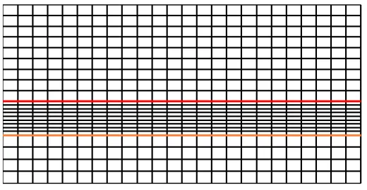
Figure 3.2: Meshing of the domain of solution Ω of the PDE (3.1). The red line represents the vessel-membrane interface Ivm _{and the orange line represents the membrane-tissue interface} _Imt_.

Notice that the spatial resolutions in the y-direction vary over each layer; further details on the selection of the spatial step size iny is provided in Section 3.2.1. In all numerical results presented in Section 3.3, we used an equispaced grid in thex-direction.

whereNt,Nm, andNvare the number of grid points used in they-direction in the tissue, membrane, and vessel layers respectively. An example of these grids for a particularDv andMv is displayed in Figure 3.3(a).

Application of this change of variables transforms the PDE (3.1) in the vessel into the variable-coefficient convection-diffusion equation

ˇ

Ct=Dv( ˇCxx+G2ξ2Cˇξξ)−vbloodCˇx+Gξ(GDv+Mv) ˇCξ, (3.3)

where ˇC(x, ξ, t) =C(x, y, t).

For clarity, and to highlight the differences between VMT solvers using the above graded mesh and those using alternate meshing strategies, we henceforth refer to any VMT method using an exponential change of variables as a Graded VMT Solver. In all the numerical simulations of the finite differences-based Graded VMT solver shown in Section 3.3, we chose G = −Dv_/8Mv _and

Nv _{= 2N}

y/5, Nm = 2Ny/5, and Nt = Ny/5, where Ny is the number of grid points in the

y-direction.

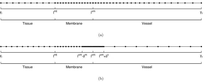
3.2.1.2 Multiple Equispaced Meshes

(37)

y_l _Imt

Ivm yr

Tissue Membrane Vessel

(a)

y_l _Imt

Ivm-δm _Ivm _Ivm₊δv y_r

Tissue Membrane Vessel

[image:37.612.117.549.82.257.2]

(b)

Figure 3.3: Grids used by the Graded and Standard VMT solvers. Figure (a) depicts the expo-nentially graded mesh given by (3.2) with G = −Dv/8Mv and Figure (b) displays the multiple equispaced meshes given by (3.4) withδm=Dv/Mv,δv =Dv/Mv.

the variable-coefficient FC-ODE solver; due to the GMRES-step, the variable-coefficient FC-ODE algorithm is more computationally expensive than its constant-coefficient counterpart. In contrast, the use of additional equispaced meshes does not depend on transformation of the constant-coefficient PDE (3.1), and so efficient numerical solution is provided by the FC-AD method with the constant-coefficient FC-ODE solver.

In detail, we make use of the discrete grids

yt:={yj=j(Imt−yl)/(Nt−1)|j = 0, ..., Nt−1},

ycm:={yj =j(Ivm−δm−Imt)/(Ncm−1)|j= 0, ..., Ncm−1},

yf m:={yj =jδm/(Nf m−1)|j= 0, ..., Nf m−1},

yf v:={yj=jδv/(Nf v−1)|j= 0, ..., Nf v−1},

ycv:={yj =j(yr−Ivm+δv)/(Ncv−1)|j= 0, ..., Ncv−1},

(3.4)

where δm _and _δv _{are selected to ensure adequate resolution of the boundary layer. For all the}

numerical results presented in Section 3.3, we choseδm₌_Dv_/Mv_, _δv ₌_Dv_/Mv _and _Nt₌_N y/5,

Ncm₌_N

y/5,Nf m=Ny/5,Nf v =Ny/5,Ncv =Ny/5.

3.2.2 ADI

(38)

Vessel Membrane Tissue

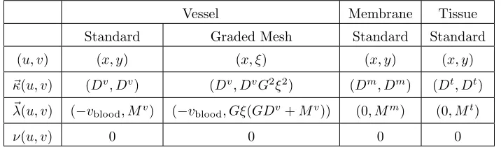
Standard Graded Mesh Standard Standard

(u, v) (x, y) (x, ξ) (x, y) (x, y)

~

κ(u, v) (Dv_{, D}v₎ _(Dv_{, D}v_G2_ξ2₎ _(Dm_{, D}m₎ _(Dt_{, D}t₎

~

λ(u, v) (−vblood, Mv) (−vblood, Gξ(GDv+Mv)) (0, Mm) (0, Mt)

[image:38.612.146.504.73.178.2]

ν(u, v) 0 0 0 0

Table 3.1: Table of coefficients and coordinates used in each layer, including both the standard equi-spaced and expontially graded meshes in the vessel. The far left column provides the corresponding notation used in Section 2.3 for the description of the ADI algorithm.

overcome this restriction, we make use of an efficient solver that does not incur a CFL condition, namely, the Alternating Directions Implicit (ADI).

Numerical solvers for the full VMT problem arise from implementation of the ADI methodology in each grid: solution of the ODEs inherent in the ADI algorithm via finite differences yield FD-based VMT solvers, while FC-based VMT solvers result from application of the FC-AD method in each grid to the associated PDE. For all the numerical results presented in Section 3.3 that were obtained from implementation of FD-based VMT solvers, we make use of the standard centered-difference finite difference scheme.

Recalling the ADI methodology previously described in Section 2.3, we note that application of the FC-AD algorithm to the VMT model depends on appropriate definition of the coordinates (u, v) and functions~κ, ~λ, ν, Q, a, b, G, and C0. From inspection we may immediately note that

the inhomogeneity Q(u, v, t) is simply 0 and the initial condition C0 is given by (3.1). However,

because of the variety of meshes and change of variables available for use in any given VMT solver, definition of the coefficient functions~κ,~λ, and ν in each layer depends on the specific combination of techniques employed. A listing of the appropriate choices of the coordinates (u, v) and coefficient functions~κ,~λ,ν required for various implementations of the VMT solver is provided in Table 3.1.

Due to the various diffusive and advective terms used in each layer, the boundary conditions at each layer interface must be treated with care to ensure a correct physical solution. Section 3.2.3 discusses the enforcement of these boundary conditions, henceforth referred to as “jump conditions”, for FD- and FC-based VMT solvers.

3.2.3 Jump conditions

(39)

3.2.3.1 FD-Based Methods

For the FD-based ADI method, satisfaction of these jump conditions is achieved through a imple-mentation combination of forward and backward finite-difference schemes at each layer. For example, and for ease of explanation, using the forward and backward Euler discretization schemes the jump conditions at the membrane-tissue interface require

−D t ht y

C_i,In ₋₁+

_Dt

ht +

Dm hm +M

t₋_Mm

C_i,In +

−D

m

hm

C_i,In₊₁= 0, (3.5)

wherehmandhtare the spatial step sizes in the membrane and tissue respectively, and C_i,In is the approximate concentration atx=hxi, y =Imt, and time tn =n∆t. The index I corresponds to

the membrane-tissue index after appropriate discretization. Note that continuity ofCis inherently enforced through the satisfaction of (3.5). The jump conditions at other interfaces are similarly enforced.

Satisfaction of the zero-flux boundary conditions at the domain boundaries is achieved through enforcement of

(C_i,n₁−C_i,n₀)/ht= 0, (C_i,Nn _y −C_i,Nn _y₋₁)/hv= 0,

where we have again approximated ∂C/∂y using the forward and backward Euler discretization schemes respectively.

For all implementations of FD-based VMT solvers presented in Section 3.3, we made use of the second-order forward and backward finite difference schemes

∂Cn i,j

∂y = 1 2h(−3C

n i,j+ 4C

n i,j+1−C

n

i,j+2) +O(h

2_), _and

∂C_i,jn ∂y =

1 2h(3C

n i,j−4C

n

i,j−1+C

n

i,j−2) +O(h 2_),

respectively, to enforce both the boundary conditions in x and y and jump conditions at each interface.

3.2.3.2 FC-Based Methods

Enforcement of the jump conditions for the FC-based solver requires additional considerations. For ease of explanation, in this section we will consider only the simplest meshing scheme: one equispaced mesh in each layer. Generalization to more complex meshing schemes may be achieved in a fairly straightforward manner.

(40)

flux across each interface, the systems determining the corresponding coefficients in each layer may not be treated seperately. Indeed, the 2×2 system shown in equation (2.18) now becomes a 6×6 system relating the coefficients in each layer as follows

             

(ht

1)

0

|yl (h

t

2)

0

|yl 0 0 0 0

ht1|Imt ht₂|_Imt −hm₁|_Imt −hm₂ |_Imt 0 0

Ft

mt(ht1) Fmtt (ht2) −Fmtm(hm1) −Fmtm(hm2 ) 0 0

0 0 hm

1|Ivm hm₂ |_Ivm −hv₁|_Ivm −hv₂|_Ivm

0 0 Fvmm (hm1 ) Fmvm(hm2) −Fvvm(hv1) −Fvvm(hv2)

0 0 0 0 (hv1)0|yr (h

v

2)0|yr

                            c1 c2 c3 c4 c5 c6               =              

−(Ct

p)

0

|yl

Cpm|Imt−C_pt|_Imt

Fm

mt(Cpm)−Ftmt(Cpt)

Cv

p|Ivm−C_pm|_Ivm

Fv

vm(Cpv)−Fvmm (Cpm)

−(Cpv)0|yr

              ,

whereF(f) =Dfy+M f is the flux in the layer specified by the associated superscript and evaluated

at the interface specified by the associated subscript.

3.2.4 Fluid-Freezing Methodology

To resolve the advection in the vessel, we begin by using a small time step, ∆t= 0.5. This presents a problem, however: because the magnitude of the diffusion in the membrane and tissue is typically taken to be extremely small, the concentration will not reach steady state in a reasonable amount of time if the time step is kept small. At the same time, if the time step is taken to be much larger, we risk being unable to resolve the advection in the vessel. To overcome this difficulty, we periodically “freeze” the concentration in the vessel and evolve only in the membrane and tissue using a large time step. Once the freezing approximation is no longer accurate, the vessel is “unfrozen” and the time-step significantly reduced. The entire system is then evolved at the reduced time step until the freezing process can be used again.

In detail, freezing occurs when the concentration in the vessel has reached a near steady state; the concentration is said to have reached a steady state in a specified layer when the maximum relative residue,

|C(x, y, tn+1₎₋_{C(x, y, t}n₎_|

|C(x, y, tn+1₎_| , (3.6)

over the relevant layer points (x, y) is smaller than a prescribed tolerance. In the remainder of this text, we denote the steady state tolerance for the concentration in the vessel, or freezing tolerance, by σf. The accuracy of the freezing approximation is determined by measuring fulfillment of the