A high resolution study of the high redshift intergalactic medium

(1)

Intergalactic Medium

Thesis by George D. Becker

In Partial Fulfillment of the Requirements for the Degree of

Doctor of Philosophy

California Institute of Technology Pasadena, California

2007

(2)

c

2007

George D. Becker

(3)

For my family,

who have supported me at every step,

and for Molly,

(4)

Acknowledgements

It is a pleasure to thank some of the many people from whom I have received support, although there are far too many to be listed here. I received early support from my un-dergraduate advisor, Bob O’Connell, who introduced me to research and encouraged me to

do my graduate work at Caltech, and from Ray Ohl, whose enthusiasm helped many in my class at UVa to pursue the sciences. While at Indiana, I was fortunate to receive additional

encouragement and direction from Mike Pierce.

Nearly all of the observations presented here were performed at the Keck telescopes in

Hawaii, and I am deeply indebted to the Keck staff for their patient assistance through many nights of observing. Closer to home, I am thankful to the staff in Robinson, particularly

Gina Armas, Gita Patel, and Diane Fujitani for making all of the practical aspects of life at Caltech easy. I am especially grateful to our systems administration team of Patrick

Shopbell, Anu Mahabal, and Cheryl Southard. Their tremendous expertise and hard work make all scientific progress in the department possible.

My thanks to Judith Mack for opening her home on many occasions - and for the flan. It has been a great pleasure to be part of an exceptional community of grad students.

Their talents are remarkable, both in astronomy and far beyond, and I have leaned a great deal from each of them. Lunches were one of the best times to reflect and relax, and I was

privileged to enjoyed the regular company of David Kaplan, Dawn Erb, Micol Christopher, Jackie Kessler-Silacci, and Naveen Reddy, as well as most of the other grad students at

different times.

Many thanks to my enjoyable and accommodating office mates: Anu Mahabal, Pranjal

Trivedi, Edo Berger, Matt Hunt, Bryan Jacoby, Laura Hainline, and Stuartt Corder. I am also grateful to the fun and always tolerant people with whom I shared a roof: Noah

Robin-son, Jon Sievers, Milan Bogosavljevic, Francis O’Donovan, Jennifer Carron, Dan Stark, and Adam Krauss.

The astronomy department’s soccer, basketball, and softball teams have been a welcome outlet, and I thank Mike Santos, Rob Simcoe, Micol Christopher, and Larry Weintraub for

organizing these. Opportunities to make music have been indispensable, and I am grateful to the Angeles Chorale and the Caltech Thursday Jazz Band for the chance to perform with

(5)

time and talent to lead the Caltech Bands. Bill is an invaluable resource for the Caltech community.

My thanks to Rob Simcoe for showing me the ropes of quasar absorption line research as I was beginning at Caltech. I am also grateful to Michael Rauch, who has been a great

source of encouragement and a reliable sounding board. I have greatly enjoyed the trips with Michael to observe in Chile, even if we had to spend hours deciding who would go first

down the mountain.

Finally, I could not have asked for a better thesis advisor than Wal Sargent. Wal

possesses an astounding wealth of knowledge, astronomical and otherwise, and I have greatly enjoyed our many conversations. I have been particularly pleased to share with Wal a love

of music. On observing runs, we seemed to agree the most on Baroque composers, but could also entertain a rare moment of jazz (when he was willing). Dinners at Merriman’s were

always a favorite (thanks, Ira). Most importantly, though, Wal provided me with every opportunity to do good science, and allowed me to find my own way with only a gentle

(6)

Abstract

We measure the spatial coherence of filamentary structures in the intergalactic medium (IGM) at z _∼ 4. The transmitted flux in the Lyα forest is significantly cross-correlated in the spectra of two pairs of QSOs at z _∼ 4 with angular separation ∆θ _∼ 30′′. This strongly suggests that some fraction of the absorbing structures span the _∼ 1 comoving Mpc separation between paired sightlines.

We further present measurements of the ionization state of the high-redshift IGM using three approaches: a search for low-ionization metal lines atz >5, a study of the evolution of

Lyα optical depths over 2.z.6, and a measurement of the UV background at 4.z.5 using the quasar proximity effect. We identify six Oisystems in the HIRES spectra of nine

QSOs with redshifts 4.9≤zQSO≤6.4. Four of these systems lie towards SDSS J1148+5251

(zQSO = 6.4). This excess at z ∼6, however, is unlikely to indicate a significantly neutral

IGM suggestive of the end of reionization, since the Oifalls over a redshift interval that also

shows transmission in Lyαand Lyβ. In contrast, we find no Oitowards SDSS J1030+0524

(zQSO= 6.30), whose spectrum shows a broad Gunn-Peterson trough. That sightline must

also be highly ionized, therefore, or else chemically pristine. The relative abundances of O,

Si, and C in the systems we detect are consistent with enrichment from Type II supernovae, with an upper limit of 30% on the amount of metals contributed by supermassive stars.

We examine the evolution of Lyα optical depth using the transmitted flux probability distribution function (PDF) in the spectra of 63 QSOs spanning absorption redshifts 1.7<

z < 5.8 to predictions from two theoretical τ distributions. For an isothermal IGM and a

uniform UV background, the optical depth distribution computed from a density model that

has been used to make claims of late reionization produces poor fits to the observed flux PDF unless significant corrections to the QSO continua are applied. In contrast, a lognormal τ

distribution fits the data at all redshifts with only minor changes in the continua. A simple linear fit to the redshift evolution of the lognormal parameters at z < 5.4 reproduces the

observed mean Lyα and Lyβ transmitted fluxes over 1.6 < z <6.2. Assuming the density field, temperature, and UV background vary slowly atz <5, this suggests that no sudden

change in the IGM due to late reionization is necessary to explain the lack of transmitted flux atz&6.

(7)

proximity effect in a sample of 16 QSOs. Accurate redshifts were obtained from Mg ii

emission lines, supplemented by estimates from the start of the Lyαforest and CO emission.

We use a new method for directly estimating the size of a QSO’s proximity region based on the observed transmitted flux distribution. The relative sizes of the proximity regions

are consistent with the expected trend in QSO luminosity, although the proximity regions around faint QSOs may be disproportionately small. Our estimate of the background H i

ionization rate, Γbg = (1.4+1.6₋_0.7)×10−12s−1, is consistent with no evolution fromz&2 based on other measurements using the proximity effect, the mean opacity of the Lyα forest, and

(8)

List of Figures

1.1 The HIRES high-z sample . . . 8

2.1 Keck/ESI spectra of Q1422+2309 and Q1422+2255 . . . 15

2.2 Keck/ESI spectra of Q1439₋0034A and Q1439₋0034B . . . 15

2.3 Lyα forest in Q1422+2309 and Q1422+2255 . . . 17

2.4 Lyα forest in Q1439₋0034A and Q1439₋0034B . . . 17

2.5 Flux correlation functions . . . 20

2.6 Distribution of pixel fluxes in Q1422+2309 and Q1422+2255 . . . 23

2.7 Distribution of pixel fluxes in Q1439₋0034A and Q1439₋0034B . . . 24

2.8 Effects of noise on the autocorrelation function . . . 27

2.9 Effects of resolution on the autocorrelation function . . . 28

2.10 Relative effects of resolution on the auto- and cross-correlation functions . 30 2.11 The z_≈3.1 C ivsystems in Q1422+2309 and Q1422+2255 . . . 34

2.12 The z≈3.4 C ivsystems in Q1439−0034B . . . 35

2.13 The z_≈1.7 Mgii systems in Q1439−0034A and Q1439−0034B . . . 38

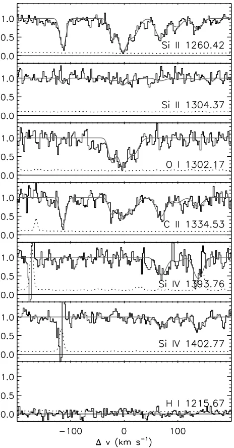
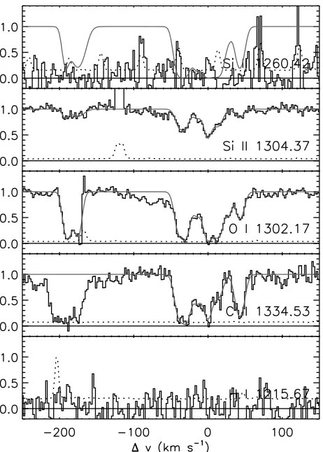
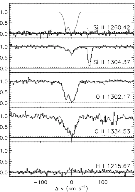
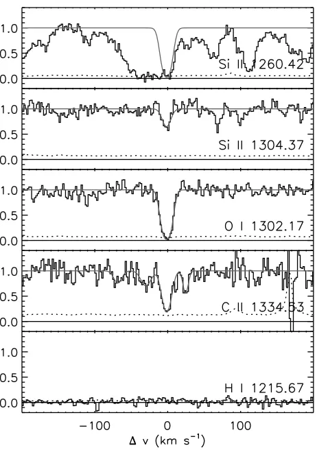
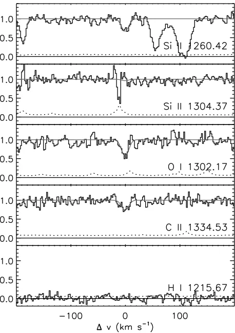
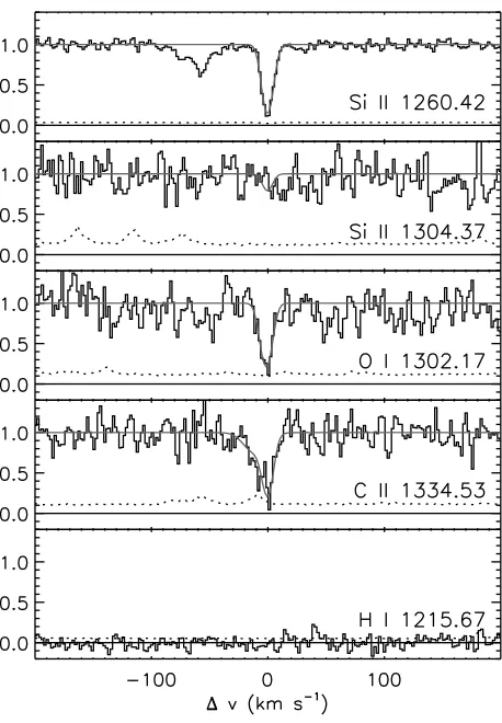
3.1 The z= 5.3364 Oi system in SDSS J0231−0728 . . . 49

3.2 The z= 5.8408 Oi system in SDSS J1623+3112 . . . 51

3.7 Sensitivity curves for O i detection . . . 58

3.8 Effective O iabsorption pathlength interval . . . 59

(12)

3.10 Upper limit on NHI for thez= 5.3364 Oisystems in SDSS J0231−0728 . 66

3.11 Upper limit on NHI for thez= 6.0097 Oisystems in SDSS J1148+5251 . 66

4.1 Fits to the Lyα flux PDFs at 4.254≤ hzi ≤5.614 . . . 85

4.2 Fits to the Lyα flux PDFs at 3.126_{≤ h}z_{i ≤}4.234 . . . 86

4.4 Fits to the Lyα flux PDFs at 2.374_{≤ h}z_{i ≤}2.643 . . . 88

4.6 Reduced χ2 _{values for PDF fits: continuum and zero point fixed . . . .} ₉₀

4.7 Reduced χ2 values for PDF fits: continuum and zero point allowed to vary 91 4.8 Continuum adjustments for PDF fits as a function of redshift . . . 93

4.9 Examples of continuum adjustments overlaid on spectra . . . 94

4.10 Lognormalτ distribution parameters . . . 95

4.11 Redshift evolution of theoreticalτ and flux distributions . . . 97

4.12 Evolution of τ_effα over 3_≤z_≤6.2 (linear) . . . 99

4.13 Evolution of τ_effα over 1.6≤z≤6.2 (logarithmic) . . . 100

4.14 Evolution of τ_effβ over 3_≤z_≤6.2 (linear) . . . 101

4.15 H iionization rates determined from flux PDFs . . . 103

4.16 Example fits to Lyα flux PDFs using a non-isothermal MHR00 model . . . 106

5.1 NIRSPEC H-band spectra of QSO Mg ii emission lines . . . 128

5.2 Proximity regions in QSO with 1h <RA<3h . . . 131

5.3 Proximity regions in QSO with 3h _<_RA_<₈h _{. . . .} ₁₃₂

5.4 Proximity regions in QSO with 8h <RA<11h. . . 133

5.5 Proximity regions in QSO with 12h _<_RA_<₂₃h _{. . . .} ₁₃₄

5.6 Theoretical flux PDFs in a QSO proximity region . . . 139

5.7 Proximity region size as a function of QSO luminosity . . . 144

5.8 Median flux in QSO proximity regions . . . 146

(13)

List of Tables

2.1 Summary of QSO Pairs Observations . . . 14

2.2 Lyα Forest Cross-Correlation Values . . . 21

2.3 Q1424+2255 Metal Systems . . . 32

2.4 Q1439−0034A Metal Systems . . . 36

2.5 Q1439₋0034B Metal Systems . . . 37

3.1 Summary of Observations for Oi Search . . . 44

3.2 Measured Properties of Oi Systems . . . 46

3.3 Abundance Measurements . . . 63

3.4 Comoving Mass Densities . . . 67

4.1 Fitted Lyα Forest Regions . . . 76

4.2 Best-Fit MHR00 Model Parameters (Isothermal) . . . 108

4.3 Best-Fit Lognormal Parameters . . . 112

(14)

4.4 Best-Fit MHR00 Model Parameters (Non-Isothermal) . . . 117

5.1 Summary of Proximity Effect Observations . . . 125

5.2 QSO Redshifts . . . 127

5.3 QSO Continuum Properties . . . 135

5.4 UV Background Measurements . . . 141

(15)

Chapter 1 Introduction

1.1 Overview

The past two decades have witnessed tremendous advances in the study of the high-redshift intergalactic medium (IGM). Sky surveys have made the detection of quasars out to z_∼6 nearly routine. At the same time, numerical simulations of large-scale structure are able to reproduce many of the observed properties of quasar absorption lines, particularly the

complex patter of H i absorption known as the Lyα forest. This concordance between

observations and simulations has secured the “cosmic web”, a self-gravitating network of

filaments, sheets, and voids, as the standard model for the IGM. The scaffolding for the web is provided by dark matter, whose evolution from a set of initial conditions can be

realistically simulated for an assumed set of cosmological parameters, given the limits set by the resolution and size of the simulation box. Baryons will tend to follow the dark

mat-ter, but are further subject to hydrodynamics, ionization, heating, and other complicating factors such as chemical and mechanical feedback from galaxies. Many properties of the

IGM are therefore difficult to determine from first principles and must be constrained ob-servationally. These include the size of absorbing structures, the intensity of the ionizing

radiation field, and the composition and distribution of heavy elements. Perhaps the largest unknowns concern the timing and mechanisms of cosmic reionization. The fact that Lyα

photons reach us from quasars out to z ∼ 6 implies that the hydrogen in the IGM was already ionized by that epoch, but how much further back reionization occurred and what

(16)

This work aims to shed light on several aspects of the evolution of the high-redshift IGM using multiple unique observations of quasars at z >4. In Chapter 2 (reprinted from the

Astrophysical Journal, v. 613, p. 61, written with W. Sargent and M. Rauch), we use two

widely spaced pairs ofz_∼4 quasars to demonstrate that absorbing structures are correlated out to at least 1 comoving Mpc. Chapters 3 and 4 utilize the first high-resolution spectra of quasars at 4.9 _≤z _≤6.4 to examine the evolution of the Lyα forest and metal lines at these epochs, and to test the plausibility of reionization atz∼6.2. In Chapter 3 (reprinted from the Astrophysical Journal, v. 640, p. 69, written with W. Sargent, M. Rauch, and

R. Simcoe), we conduct a search for Oias a potential tracer of chemically enriched, neutral

gas. In Chapter 4 (submitted to the Astrophysical Journal, written with M. Rauch and

W. Sargent), we test the ability of two models for the distribution of Lyα optical depths to produce the observed transmitted flux distribution. The evolution of the optical depths is

then used to explain the disappearance of transmitted flux atz >6. Finally, in Chapter 5, we employ a large set of quasars with accurate Mg ii redshifts to measure the intensity of

the metagalactic ionizing background at 4.z.5 using the quasar proximity effect.

1.2 Scientific Background

Many of the basic properties of the IGM have been established since the late 1970’s and early

1980’s, when sensitive detectors became available for use on 4-5m telescopes. Sargent et al. (1980) demonstrated that the numerous Lyα absorption lines seen in quasar spectra are

associated with weakly clustered, low density, photoionized parcels of intergalactic gas with temperatures ofT _∼104 _{K. More recently, high-resolution spectrographs on 8-10m}

ground-based telescopes (in particular, HIRES on Keck and UVES on the VLT) have allowed the

z > 2 Lyα forest to be studied with great sensitivity (e.g., Hu et al. 1995). Ultraviolet

spectrographs on board the space-based telescopes have, meanwhile, opened up the IGM down to z = 0 (e.g., Penton et al. 2000). With a long baseline over which to study the

evolution of the Lyα forest, statistics such as the distributions of H icolumn densities, the

distribution of Doppler widths, and the flux power spectrum are now established out to

z∼5.

During the 1980s, Lyα absorbers were primarily thought of as isolated clouds that

(17)

simulations capable of following the growth of large-scale structure (e.g., Cen et al. 1993), an interconnected network of dark matter and baryons formed from the gravitational collapse of

density perturbations left over from the Big Bang has become the standard paradigm. The “cosmic web” (Bond & Wadsley 1997) model of the IGM has proven remarkably successful

in reproducing the observed properties of the Lyα forest, such that synthetic spectra from simulations are, in many (though not all) ways, indistinguishable from real data. This

agreement has been one of the great successes in the study of the high-redshift Universe. The gravitational collapse model has been the backdrop for a number of experiments

that use the IGM as a cosmic laboratory. The opacity of the forest can be used to set limits on the baryon density (Rauch et al. 1997). The temperature-density relation of the

IGM can be measured from the distribution of observed line widths (Schaye et al. 2000; McDonald et al. 2001). Correlations in the Lyα forest probe density fluctuations down to

scales of . 1 comoving Mpc. When combined with measurements out to horizon scales from the cosmic microwave background (CMB), these correlations place tight constraints

on the amplitude and slope of the matter power spectrum (e.g., Spergel et al. 2003; Viel et al. 2006). The better we understand the fundamental properties and evolution of the

IGM, the more reliably such tests can be performed.

1.2.1 The Metagalactic Ionizing Background

Most of the evolution of the Lyαforest can be explained by the expansion of the Universe, the gravitational collapse of large-scale structures, and the evolution of the ionizing

back-ground (e.g., Dav´e et al. 1999). Among these factors, the ionizing backback-ground is the most difficult to constrain theoretically, as it depends not only on the rates of star formation

and quasar activity, which are highly non-linear processes, but on the fraction of ultraviolet photons that escape from ionizing sources into the IGM (e.g., Steidel et al. 2001). Much of

the integrated UV output of star-forming galaxies and quasars will come from faint sources, which require deep observations to detect at high redshift (e.g., Hunt et al. 2004; Yan &

Windhorst 2004). Furthermore, in a highly ionized Universe, the mean free path of ionizing photons will be set by the number density of optically thick Lyman limit systems (absorbers

with H i column densities N_H_I ≥ 1017.2 cm−2). Numerical simulations are generally not

(18)

Given these factors, independent estimates of the UV background are valuable both for de-termining the ionization state of the IGM and for constraining models of galaxy and quasar

formation.

In principle, the intensity of the UV background can be determined from the mean level

of transmitted flux in the Lyαforest. In creating artificial quasar spectra from simulations, the background level is typically ‘tuned” such that the optical depths in the simulation

produce transmitted flux levels that match the real data. However, the hydrogen neutral fraction, and hence the Lyα optical depth, also depends on the density and temperature

of the gas. The non-linear relationship between optical depth and transmitted flux further means that the mean transmitted flux will depend on thedistributionof optical depths (e.g.,

Songaila & Cowie 2002). For a given simulation, this will depend not only on the density distribution, which is sensitive to the cosmological parameters, but also on assumptions

about the thermal state of the gas. It is common to assume either a uniform temperature or a simple monotonic relationship between temperature and density. Radiative transfer

effects, however, may complicate the temperature distribution considerably (Bolton et al. 2004).

In order to disentangle the ionization rate from the density and temperature of the gas, independent measurements of the ionizing background must be made. At z _≈ 0 the UV background can be estimated from the truncation of Hidisks in spiral galaxies (e.g., Sunyaev

1969; Dove & Shull 1994). Ratios of metal species with different ionization potentials can be used to constrain the strength and shape of the radiation field, assuming that the

species populations are set by photoionization (e.g., Songaila 1998). However, strong metal absorption systems are typically associated with galaxies. (e.g., Boksenberg et al. 2003).

Their ionization state may therefore depend more on the local ionizing output of the galaxy than on a truly metagalactic background.

The quasar proximity effect offers an alternate means of measuring the ionizing back-ground using the Lyα forest. The amount of absorption in the forest generally increases

with redshift. However, near a quasar, the absorption tends to decrease. This is generally attributed to locally enhanced photoionization by the quasar itself. Knowing the

(19)

Bajtlik et al. 1988). The most successful applications of the proximity effect have been

at z < 4, where individual Lyα lines can be easily identified and large samples of quasar

spectra can be used to overcome the variance in the forest (e.g., Scott et al. 2000, 2002). At higher redshifts the measurements have been more sparse. In addition, previous studies

have not demonstrated that the extent of the proximity region depends correctly on the luminosity of the quasar, and hence that the values obtained for the UV background are

accurate. Proximity effect measurements would be particularly valuable atz >4, where the ionizing output of galaxies and quasars becomes increasingly difficult to measure directly.

A consensus between galaxy/quasar counts, the mean transmitted flux in the Lyα forest, and the proximity effect would imply a genuine understanding of the ionization state of the

high-redshift IGM.

1.2.2 Reionization

As pointed out by Gunn & Peterson (1965), Scheuer (1965), and Shklovskii (1965), an expanding Universe filled with neutral hydrogen would produce a tremendous Lyα optical

depth (τLyα ∼105). The fact that we observe transmitted flux in the Lyα forest, therefore,

implies that the IGM must now be highly ionized. Following recombination at z _≈ 1100, when the Universe transitioned from being predominantly ionized to being predominantly neutral, the IGM would have remained opaque to UV photons until enough luminous sources

were formed that were able to reionize the vast majority of the hydrogen (and later helium). Determining when and how reionization occurred is one of the primary challenges of modern

cosmology, with implications both for the nature of the first luminous sources and for the subsequent growth of small-scale structure.

Observations of the cosmic microwave background (CMB) provide an upper limit on the redshift of reionization. Thomson scattering by free electrons produces linear polarization

in the CMB, which can be used to infer the total electron optical depth to the surface of last scattering. A higher τe would mean that CMB photons had encountered greater

numbers of free electrons, which would require an earlier reionization. The most recent CMB measurements indicate that τe ∼0.09 (Spergel et al. 2006). If reionization occurred

all at once, than this would imply a reionization redshift of zreion∼11. A more prolonged

(20)

High-redshift quasar can be used as a second probe of reionization. In the past seven years, the Sloan Digital Sky Survey has uncovered significant numbers of quasars out to

z= 6.4 (Fan et al. 2006b, and references therein). The absence of complete Lyαabsorption (so-called “Gunn-Peterson troughs”) at z <6 implies that the Universe was already highly

ionized one billion years after the Big Bang. However, the discovery of extended absorption troughs in the spectra of the highest-redshift objects has led to claims that reionization

may have ended as late asz∼6 (Djorgovski et al. 2001; Becker et al. 2001; Fan et al. 2002, 2006a). As noted above, a trace amount of neutral hydrogen is sufficient to produce a large

Lyα optical depth. Therefore, the rapid evolution of transmitted flux at z > 5.7, rather than the mere appearance of Gunn-Peterson troughs, has been the primary evidence for

reionization lasting until z∼6 (e.g., Fan et al. 2006a).

Late reionization remains strongly debated, however. Perhaps the best evidence against

a significantly neutral IGM at z ∼ 6 is the transmitted Lyα, Lyβ, and Lyγ flux seen towards the highest-redshift known quasar, SDSS J1148+5251 (z= 6.42) (Oh & Furlanetto

2005; White et al. 2005). In addition, no large change is seen in the luminosity function or emission line profiles of Lyα-emitting galaxies between z _∼5.7 and z _∼6.5 that would suggest absorption by a highly-neutral IGM atz >6 (e.g., Malhotra & Rhoads 2004; Hu & Cowie 2006). Theoretically, late reionization remains a flexible issue. A combination of the

clustering of ionizing sources, the uneven growth of ionized bubbles, and the inhomogeneity of the IGM can be invoked to accommodate nearly all of the current observations, either in support of or against late reionization (e.g., Wyithe & Loeb 2004a; Lidz et al. 2006b;

Furlanetto et al. 2006). New types of observations are therefore needed to clarify whether dramatic changes in the IGM are occuring atz_∼6.

1.3 Thesis Outline

To address these issues, we have obtained a variety of unique moderate- and high-resolution

spectra of quasars at z & 4. In Chapter 2, we examine ESI spectra of two sets of quasar pairs at z _∼ 4 with angular separation ∆θ _≈ 30′′. We demonstrate that the transmitted flux is significantly correlated between paired sightlines, which implies that filaments in the IGM are coherent on scales of > 1 comoving Mpc. We further investigate the effects

(21)

cross-correlation functions, a measurement that can be used to determine the cosmological constant. We conclude that spectral resolution must be carefully accounted for when making

this comparison.

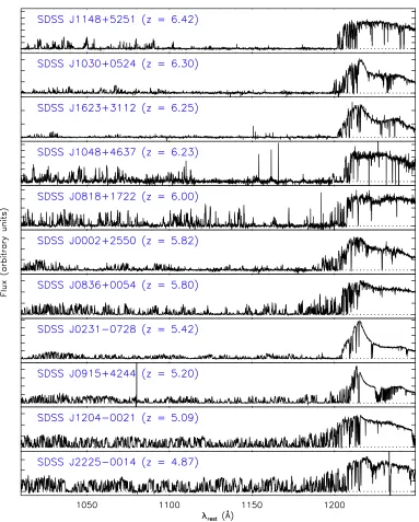
Much of this work utilizes a new set of HIRES spectra of 11 quasars at 4.9 _≤z _≤6.4 (Figure 1.1). These are the first high-resolution spectra of any quasars atz >4.8, giving us an unprecedented view of the Lyαforest and metal absorption lines at these redshifts. The

observations were made possible due largely to the recently upgraded detector on HIRES. Even so, many of these objects are at the sensitivity limits of current instruments, and the

total sample represents over 100 hours of integration.

In Chapter 3, we use the HIRES high-z sample to search for Oi absorption as a probe

of neutral gas at z > 5. We uncover six systems, four of which lie towards our highest-redshift objects, SDSS J1148+5251 (z= 6.42). We demonstrate that this is a statistically

significant excess, but that it is unlikely to indicate a highly-neutral IGM since this sightline also shows Lyα and Lyβ transmission over the same redshift interval as the O i. We use

the lack of Oi detected towards SDSS J1030+0524 (z= 6.30) to argue that that sightline

must be highly ionized, despite the presence of an extended Gunn-Peterson trough, or else

chemically pristine. We further show that the relative metal abundances in the six O i

systems are consistent with enrichment from Type II supernovae, rather than hypothetical

supermassive stars.

In Chapter 4, we combine our high-z sample with HIRES data for a large number of quasars at 2.0 _≤ z _≤ 4.7 to study the evolution of Lyα optical depth from z _∼ 2 to the proposed epoch of reionization. We compare the observed flux probability distribution function (PDF) to predictions from an IGM model that has been used to infer a drop in

the Hi ionization rate atz∼6. We find that the agreement is generally poor unless large

corrections to the quasar continua are made. In constant, we show that a simple lognormal

optical depth distribution provides a good fit to the observed flux PDF at all redshifts. We further show that a steady evolution in the lognormal τ distribution reproduces the

evolution in the mean transmitted flux over 1.6< z < 6.2. We use this fact to argue that if the evolution of transmitted flux at z <5 reflects slowly-varying conditions in the IGM,

(22)

[image:22.612.134.517.127.604.2]

Figure 1.1 The HIRES high-zsample. Spectra are plotted as a function of rest wavelength.

(23)

In Chapter 5, we use the quasar proximity effect to measure the UV background at 4.z.5. These are the first proximity effect measurements atz >4 using a large number of quasars. We measure accurate systemic redshifts using infrared spectra of Mgiiemission

lines. In order to deal with line blending in the Lyα forest at z > 4, we present a new

method for determining the size of a quasar’s proximity region based on the distribution of transmitted fluxes near the quasar redshift. We also test the photoionization model

of the proximity effect by comparing the proximity regions sizes of quasars with different luminosities. We find that proximity region size has roughly the correct dependence on

quasar luminosity, but with a large scatter. We further show that our value for the H i

ionization rate is consistent with no evolution in the UV background over 2. z. 5, and that proximity effect measurements at high redshift are consistent with the opacity of the Lyα forest and the combined ionizing output of star forming galaxies and quasars.

(24)

Chapter 2 Large-Scale Correlations in the Ly

α

Forest at

z

= 3

₋

4

1

Abstract

We present a study of the spatial coherence of the intergalactic medium toward two pairs of

high-redshift quasars with moderate angular separations observed with Keck/ESI, Q1422 +2309A & Q1424+2255 (zem ≈3.63, ∆θ= 39′′) and Q1439−0034A & B (zem ≈4.25, ∆θ

= 33′′). The cross-correlation of transmitted flux in the Lyα forest shows a 5−7σ peak at zero velocity lag for both pairs. This strongly suggests that at least some of the absorbing

structures span the 230−300h−₇₀1 proper kpc transverse separation between sightlines. We also statistically examine the similarity between paired spectra as a function of transmitted

flux, a measure which may be useful for comparison with numerical simulations. In investi-gating the dependence of the correlation functions on spectral characteristics, we find that

photon noise has little effect for S/N & 10 per resolution element. However, the agree-ment between the autocorrelation along the line sight and the cross-correlation between sightlines, a potential test of cosmological geometry, depends significantly on instrumental

resolution. Finally, we present an inventory of metal lines. These include a a pair of strong Civsystems atz≈3.4 appearing only toward Q1439B, and a Mgii+ Feiisystem present

toward Q1439 A and B atz_≈1.68.

1_{Originally published in} _{The Astrophysical Journal}_{, v. 613, p. 61; written with W. L. W. Sargent and}

(25)

2.1 Introduction

Multiply-imaged lensed quasars and close quasar pairs provide valuable probes of structure in the intergalactic medium. By comparing the absorption patterns in the spectra of ad-jacent quasar images one can gauge the similarity in the underlying matter distributions

along the lines of sight and hence constrain the sizes of absorbing structures. Previous studies at small separations (∆θ.10′′) have typically provided lower limits to the scale of Lyα absorbers over a wide range in redshift, with weak upper constraints of∼400 comov-ing kpc derived by assumcomov-ing spherical clouds (Weymann & Foltz 1983; Foltz et al. 1984;

McGill 1990; Smette et al. 1992; Dinshaw et al. 1994; Bechtold et al. 1994; Bechtold & Yee 1995; Smette et al. 1995; Fang et al. 1996). Observations of pairs at wider separations

(∆θ ≈ 0.5′ −3′) have shown evidence that some Lyα absorbers span & 1 comoving Mpc (Petitjean et al. 1998; Crotts & Fang 1998; D’Odorico et al. 1998, 2002; Young et al. 2001;

Aracil et al. 2002) and possibly up to 30 comoving Mpc (Williger et al. 2000).

The majority of studies on lensed quasars and quasar pairs have relied on matching

individual absorption lines between spectra. High-resolution spectra (FWHM.20 km s−1) are required to completely resolve these features, however. In addition, the crowding of lines

in the high-redshift Lyα forest often prevents the identification of single absorbers. Liske et al. (2000) instead used transmitted flux statistics as a function of smoothing length to

identify significantly underdense or overdense regions. Their analysis of paired sightlines at z_∼2₋3 suggests that absorbing structures may span&3 comoving Mpc. An alternate ap-proach reflecting the continuity of the underlying density field is to compute the correlation of transmitted flux along parallel lines of sight. This robust statistic is quickly computed

and can be easily compared to numerical simulations of large-scale structure (e.g., Viel et al. 2002).

As an extension to studying the matter distribution, correlations in the Lyαforest have been proposed as a tool for constraining the cosmological constant through a variant of

the Alcock-Paczy´nski test (Alcock & Paczynski 1979). The Alcock-Paczy´nski test takes advantage of the fact that, for a homogeneous sample of objects, the characteristic radial

and transverse sizes should be equal. In the case of the Lyα forest, one can compare the correlation length of absorbing structures along the line of sight to the correlation length

(26)

sight is simply given by their redshifts,

∆vk = ∆z

1 +zc . (2.1)

In contrast, the transverse velocity separation, ∆v⊥, between objects at redshift z with

angular separation ∆θdepends on the cosmological parameters implicit in the Hubble con-stant,H(z), and angular diameter distance,DA(z), as

∆v⊥=H(z)∆l=H(z)DA(z)∆θ , (2.2)

where ∆lis the proper linear separation. One approach to exploiting the difference between

∆vkand ∆v⊥is to directly compare the autocorrelation of transmitted flux along single lines of sight to the cross-correlation between spectra of sources at a variety of angular separations

(Hui et al. 1999; Lidz et al. 2003). An alternate method compares observed cross-correlations to those determined from linear theory (McDonald & Miralda-Escud´e 1999) or from artificial

spectra drawn from numerical simulations (Lin & Norman 2002). Recently, Rollinde et al. (2003) found agreement between the cross-correlations and autocorrelations among spectra

of severalz ∼2 quasar pairs over a wide range in separation (although see the discussion on spectral resolution below). In the future, large surveys such as the Sloan Digital Sky

Survey (York et al. 2000) should greatly increase the number of quasar pairs available for such studies.

We present results for two pairs of quasars at a novel combination of high redshift and moderate separation. The closely separated A and C images (∆θ = 1.′′3) of the bright

z = 3.63 lensed system Q1422+2309 (Patnaik et al. 1992) have been previously exam-ined by Rauch et al. (1999, 2001a) and Rauch et al. (2001b). Adelberger et al. (2003)

recently discovered an additional faint source, Q1424+2255 (z = 3.62) (therein referred to as Q1422b), at a separation ∆θ= 38.′′5 from the lensed system. In this study, we compare

the sightlines toward Q1422+2309A (herein referred to as Q1422) and Q1424+2255 (herein referred to as Q1424 to avoid confusion with the B image of Q1422). We additionally

(27)

us to study the transverse properties of the Lyα forest and intervening metal systems over a large pathlength. Our results should provide a valuable resource for comparison with

numerical simulations of large-scale structure.

The remainder of the paper is organized as follows: In_§2.2 we present our observations together with a general overview of the data. We compute the flux correlation functions in the Lyαforest in_§2.3 and statistically examine the similarity between sightlines as a function of flux. In §2.4 we analyze the effects of photon noise and instrumental resolution on the correlation functions. Finally, we present an inventory of unpublished metal absorption

systems presented in§2.5. Our results are summarized in §2.6.

Throughout this paper we adopt Ωm= 0.3, ΩΛ= 0.7, andH0 = 70 km s−1 Mpc−1.

2.2 The Data

Our observations are summarized in Table 2.1. We observed all four quasars under good to excellent seeing conditions over the period 2000 March to 2002 June using the Keck

Echel-lette Spectrograph and Imager (ESI) (Sheinis et al. 2002) in echelEchel-lette mode. Additional observations of Q1424 were provided by C. Steidel while additional observations of Q1439A

were provided by L. Hillenbrand. All exposures were taken at the parallactic angle except for one exposure of Q1439B at an airmass near 1.0, where chromatic atmospheric dispersion

is only a minor concern.

The raw CCD frames for Q1422, Q1439A, and Q1439B were processed and the 2-D

echelle spectra extracted using the MAKEE software package. Reduction of Q1424 data was performed using a suite of IRAF scripts, as described in Adelberger et al. (2003). For each

night we used the extracted orders from at least one standard star (Feige 34, BD+284211, and/or HZ 44) to determine an instrumental response function with which to derive relative

flux calibrations. The calibrated orders of all exposures from all nights were then converted to vacuum heliocentric wavelengths and combined to produce a single continuous spectrum

per object (Figures 2.1 and 2.2). We use a binned pixel size of 20 km s−1. Normalized spectra were produced by fitting continua to the final reduced versions.

The majority of observations were made using a 0.′′75 slit. However, inspection of the spectra extracted from exposures taken with different slits widths revealed very little

(28)

Table 2.1. Summary of QSO Pairs Observations

Object Datea _{Exp. time} _FWHMb

(s) (km s−1₎

Keck/ESI

Q1422+2309A 2000 Mar 03-04 1200c _∼₅₅

Q1424+2255 2000 Mar 03 – 2001 Apr 21 44900d _∼₅₅

Q1439−0034A 2001 Jan 26 – 2002 Jun 10 8000e _∼₅₅

Q1439−0034B 2001 Apr 19 – 2002 Jun 10 42400f _∼₅₅

Keck/HIRES

Q1422+2309A 1998 Jan 30 – 1998 Apr 15 31600g _4.4

a_{Interval over which observations were made.} b_{Spectral resolution.}

c_{600 s with 0.}′′_{75 slit, 600 s with 1.}′′_{0 slit.}

d_{43100 s with 0.}′′_{75 slit (including 20900 s by C. Steidel), 1800 s with}

1.′′_{0 slit.}

e_{5000 s with 0.}′′_{75 slit, 3000 s with 0.}′′_{5 slit (L. Hillenbrand).}

f_0.′′_{75 slit.}

(29)

[image:29.612.131.519.100.321.2]

Figure 2.1 Keck/ESI spectra covering the rest wavelength region from Lyβ to Civin Q1422

(top) and Q1424 (bottom). Spectra have been binned in wavelength using 40 km s−1 pixels for display. Contamination from the [O i] λ5577 skyline can be seen in the spectrum of

[image:29.612.129.521.455.675.2]

Q1424.

(30)

a measured spectral resolution FWHM = 55 km s−1. The final ESI spectra for Q1424, Q1439A, and Q1439B have typicalS/N _≈13₋30 per resolution element in the Lyα forest, while Q1422 has S/N ≈150.

We restrict our analysis of the Lyα forest to the the wavelength region between each

quasar’s Lyα and O vi emission lines. To avoid a proximity effect from the quasar, we

include only those pixels at least 10,000 km s−1 _{blueward of the quasar’s Lyα}_{emission. We}

further include only pixels at least 1,000 km s−1 redward of Lyβ and Oviemission to avoid

any confusion with the Lyβ forest or intrinsic O vi absorption. For Q1422 and Q1424 this

yields a redshift interval ∆z = 0.50 with mean redshift hzi = 3.22. For Q1439 A and B, ∆z= 0.58 and _hz_i= 3.79. Due to the high redshift of Q1439 A and B, the Lyα forest in the spectra of these sources extends over the strong night sky lines [O i] λ5577 and Na i

λ5890,5896. In our analysis, we exclude the narrow (2₋3 ˚A) regions around these lines.

A visual comparison of the Lyα forest in the paired spectra suggests that the most striking similarity occurs among the strongest absorption features (see Figures 2.3 and

2.4). These regions often appear to be similar along adjacent lines of sight, as do regions where the absorption is nearly zero (possible “voids” relatively free of absorbing material).

Matches among intermediate strength features are less obvious, which suggests that the structures giving rise to those lines may not be as coherent over the separation between

sightlines. Many strong lines and regions of nearly zero absorption that do not coincide between spectra, however, can also be identified. The alignment of a subset of features may occur purely by chance.

Our spectral coverage also allows us to investigate the extent to which metal systems span parallel lines of sight. Two strong C iv systems appear toward Q1439B at z ≈ 3.4,

separated by 1700 km s−1. Each system has a large rest equivalent width,Wrest(1548)∼1.5

˚

A. No Civappears at this redshift toward Q1439A, however. In contrast, a low-ionization

system containing Mgii and Feii does appear along both sightlines atz≈1.68, separated

by only _∼ 400 km s−1_{. A single, extended absorber responsible for the low-ionization}

features would have a linear size&280h−₇₀1 proper kpc. These lines may alternatively arise from the chance intersection of separate, clustered absorbers. Weaker C ivsystems appear

(31)

[image:31.612.133.521.120.321.2]

Figure 2.3 A representative section of the Lyα forest in the normalized spectra of Q1422 (grey line) and Q1424 (black line).

(32)

systems in the appendix.

In order to assess the effect of spectral characteristics on our Lyα forest results, we

additionally employed a deep, high-resolution spectrum of Q1422+2309A. Observations were made with the Keck High Resolution Echelle Spectrometer (HIRES) (Vogt et al. 1994)

using a 0.′′574 slit. This yields a spectral resolution FWHM = 4.4 km s−1. Reductions were performed as described Rauch et al. (2001a). In addition to the data from that work,

which used the red cross-disperser only, we include subsequent exposures taken with the UV-blazed cross-disperser installed to provide additional coverage of the Lyα forest. The

final spectrum was binned to give a constant velocity width for each pixel of 2.1 km s−1, with a typical S/N per resolution element of 50₋90.

2.3 Comparison of Sightlines

2.3.1 Correlation Functions

The correlation of transmitted flux in the spectra of closely separated quasars provides a simple means of quantifying the degree of similarity in the matter distribution along

adjacent sightlines. We define the un-normalized correlation,ξ, of the spectra of two sources separated on the sky by an angle ∆θas

ξ(∆θ,∆v_k) = 1

N

X h

F(∆θ, v_k+ ∆v_k)₋F¯(∆θ)i hF(0, v_k)₋F¯(0)i, (2.3)

whereF is the continuum-normalized flux, ¯F(∆θ) and ¯F(0) are the mean fluxes along the two sightlines, vk is the line-of-sight velocity, ∆vk is the longitudinal velocity lag, and N

is the total number of pixels in each spectrum within the region of interest. The sum is performed over all available pixels at a given velocity lag, of which there will be

npix(∆vk) =N −

∆vk δvpix

(2.4)

for a pixel sizeδvpix. The normalized correlation value can be computed by dividing

equa-tion (2.3) by the standard deviaequa-tion in each input spectrum.

We have chosen a pixel size for the combined spectra to give roughly 3 pixels/resolution

(33)

the correlation will be insensitive to pixel size so long as the spectrum is well sampled. The increase in the sum created by using a larger number of smaller pixels will be offset by the

increase in N so long as there are &2 pixels/resolution element. Using pixels larger than the spectral resolution will introduce smoothing effects (see_§2.4).

In order to assess the coherence of absorbing structures across adjacent sightlines, we compute the cross-correlation of transmitted flux in the Lyα forest in the spectra of our

quasar pairs. As a reference, we also determine the autocorrelation, ξ(0,∆vk), along lines of sight toward individual objects. At these high redshifts, HiLyα absorption will strongly

dominate over contaminating absorption from lower-redshift metals such as Civand Mgii.

The correlation functions should therefore accurately reflect the distribution of neutral

hy-drogen to within the present measurement errors. All correlations are computed in single-pixel steps, which are 20 km s−1 _{for the ESI data. Figure 2.5 displays the autocorrelation}

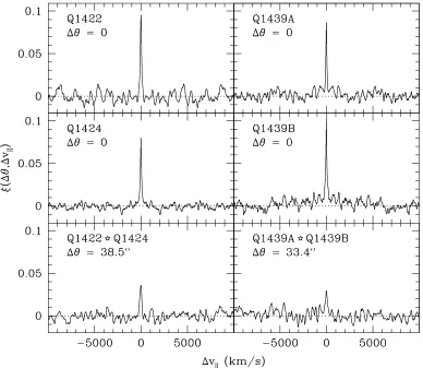
function for each quasar along with the cross-correlation functions between adjacent sight-lines. Both in the case of Q1422/Q1424 and Q1439A/B, a clear peak in the cross-correlation

at zero lag indicates a genuine similarity between sightlines.

Undulations in the correlation functions arising from the chance superposition of

unre-lated lines constitute the dominant source of uncertainty in the peak values (see discussion on photon noise below). Pixel-to-pixel variations in the correlations are themselves clearly

correlated. We find, however, that the overall distributions of values away from the central peaks are very nearly Gaussian. We therefore take the standard deviation of pixels in the “noise” region, which we define to be where 2000 km s−1 _{≤ |}_∆v

k| ≤ 18000 km s−1, as the 1σ error in a correlation peak value. In this region we expect no underlying signal, however the correlation is still computed from at least half of the available pixels. Since the

sum in equation (2.3) is computed over fewer pixels as the velocity lag increases, yet the factor 1/N remains constant, the amplitude of the noise features will tend to diminish as

q

npix(∆vk), wherenpix(∆vk) is the number of pixels included in the sum in equation (2.3) at lag ∆v_k. Therefore, in order to match the amplitude of the noise at ∆v_k = 0, we

multi-ply the correlation at each lag by a scale factorsbefore computing the standard deviation, where

s=

s

npix(0)

npix(∆vk) =

s

N

N₋∆vk/δvpix

. (2.5)

(34)

[image:34.612.132.520.176.513.2]

Figure 2.5 Flux correlation functions computed from the Lyαforest plotted vs. longitudinal velocity lag. Top four panels: Autocorrelation functions for Q1422 (top left), Q1424 (middle

left), Q1439A (top right), and Q1439B (middle right). Negative velocity lags have been

included for consistency. Bottom panels: Cross-Correlation functions for Q1422/Q1424

(35)

Table 2.2. Lyα Forest Cross-Correlation Values

QSO Pair ∆θa _z Lyα

b _∆lc _∆v

⊥d ξ(∆θ,0)

h−701 proper kpc km s−1 Un-normalizede Normalizedf

Q1422/Q1424 38.′′₅ _2.965₋_3.466 ₂₈₃₋₂₉₈ _97.8 _0.0358_±_0.0049 _0.412_±_0.057

Q1439A/B 33.′′₄ _3.496₋_4.075 ₂₃₀₋₂₄₅ _96.3 _0.0296_±_0.0057 _0.319_±_0.062

a_{Angular separation of the QSO pair.}

b_{Redshift interval used in computing the correlation values for the Lyα}_forest.

c_{Linear separation between the lines of sight for the given redshift interval, computed for Ω}

m = 0.3,

ΩΛ= 0.7, andH0= 70 km s−1Mpc−1.

d_{Transverse velocity separation between the lines of sight for our adopted cosmology at the mean redshift}

in the given interval.

e_{Cross-Correlation at zero lag computed from equation (2.3).}

f_{Cross-Correlation at zero lag computed from equation (2.3) divided by the standard deviation of the Lyα}

forest flux in each input spectrum.

where at least half of the ∼1800 Lyα pixels in each spectrum overlap limits sto at most

√

2. For the range in velocity lag shown in Figure 2.5,s <1.2.

Our results for the cross-correlations are summarized in Table 2.2. Using the above estimate for the error, the peak in the cross-correlation for Q1422/Q1424 (Q1439A/B) is

significant at the 7σ(5σ) level. This strongly suggests coherence in the absorbing structures on the scale of the 230₋300 h−₇₀1 proper kpc transverse separation between sightlines. The marginal consistency of the peak values with one another likely reflects the similarity in sightline separation and redshift for the two quasar pairs. The zero-lag values of the

autocorrelations, which give the variance in the flux for these sections of the Lyα forest, are 0.0950 for Q1422, 0.0796 for Q1424, 0.0862 for Q1439A, and 0.1000 for Q1439B. Thus,

the normalized cross-correlation peaks are 41.2±5.7% for Q1422/Q1424 and 31.9±6.2% for Q1439A/B.

2.3.2 Flux Distributions

The flux cross-correlations demonstrate that at least some Lyα absorbers span the separa-tion between our paired lines of sight. It does not, however, indicate whether the similarity

(36)

Lyα forest at z∼4, together with the present spectral resolution, greatly inhibits a study of individual lines. We are, however, able to look at the agreement between absorption

features on a pixel-by-pixel basis.

Our goal is to determine whether the similarity in flux between paired spectra depends

on the amount of absorption for an individual pixel. First, we first select those Lyα forest pixels in one spectrum (Q1422 or Q1439A) whose flux falls within a specified range. We

then identify the pixels in the companion spectrum with matching wavelengths and compute their flux distribution. Comparing the distribution in this subsample to that in all Lyα

forest pixels in the companion spectrum allows us to evaluate whether there exists an overabundance of pixels in the specified flux range relative to that expected on random

chance.

The results for Q1422/Q1424 and Q1439A/B are shown in Figures 2.6 and 2.7,

respec-tively. Each panel shows the normalized distribution of Q1424 or Q1439B pixels in the indi-cated subsample along with the distribution of all Lyα forest pixels in that spectrum. The

range of flux in Q1422 or Q1439A for each subsample is chosen to be significantly larger than the typical flux uncertainty. In each case, we compute the two-sided Kolmogorov-Smirnov

statistic, which is the maximum difference between the cumulative fractions of pixels in the subsample and of all pixels in the forest, along with the associated likelihood of randomly

obtaining a smaller statistic than the one observed. The number of pixels in each subsample is also shown.

The clearest results occur at extreme levels of absorption. Pixels in Q1422 (Q1439A)

either near saturation,F <0.2, or near the continuum,F >0.8, tend to strongly coincide with pixels of similar flux in Q1424 (Q1439B). Intermediate flux pixels appear to be less

strictly matched, with the exception of pixels in Q1422 with 0.4 < F < 0.6. For certain subsamples, namely 0.6< F <0.8 in Q1422 and 0.4< F <0.6 in Q1439A, the distribution

of fluxes in the companion spectrum is consistent with a random selection. This seems to confirm the visual appraisal that strong absorbers and regions relatively free of absorbing

material tend to span adjacent lines of sight more readily than do absorbers of intermediate strength.

(37)

Figure 2.6 Distributions of continuum-normalized pixel fluxes in the Lyαregion of Q1424 as a function of the flux in Q1422. Unshaded histograms show the flux probability distribution

for the subsample of pixels in Q1424 corresponding in wavelength to those pixels in Q1422 that have fluxes in the indicated range. Shaded histograms show the probability distribution

for all Q1424 pixels in the Lyα region. For each range of flux in Q1422, the two-sided Kolmogorov-Smirnov statistic for the subsample and full sample of Q1424 flux values is

presented along with the associated likelihood, expressed as a percent, of obtaining a higher value if the the two samples were drawn from the same distribution. The number of pixels

(38)

(39)

create clusters of pixels with low absorption near the same wavelength in pairs of spectra. Similarly, errors in sky-subtraction that are repeated between spectra might create false

coincidences of pixels near zero flux. Multiple independent continuum fits resulted in typ-ical differences of _∼ 10% in flux on scales of _∼ 100 ˚A. We likewise find no evidence for large systematic errors in the sky subtraction. Given that the resulting uncertainties are significantly smaller than the range in flux used to define a subsample in Figures 2.6 & 2.7,

these effects should only be a minor concern.

We stress that comparing transmitted fluxes does not strictly yield a clear physical

interpretation. Pixels of intermediate flux commonly occur along the wings of strong fea-tures. They will therefore tend to cluster less readily than pixels near the continuum or

near saturation, especially if the strong lines shift in velocity between spectra. Moreover, agreement in flux does not necessarily indicate agreement in optical depth. Since

trans-mitted flux decreases exponentially with optical depth, τ, the difference in flux for a given fractional change inτ will depend on the value ofτ itself. For a small characteristic change

between sightlines, ∆τ /τ ≪ 1, the greatest scatter in flux is expected for τ ∼ 1, with the scatter decreasing as τ _→ 0 or as τ _{→ ∞}. It is, therefore, unclear whether the enhanced agreement in flux among pixels with flux near the continuum or near saturation indicates that the corresponding gas is more homogeneous on these scales than the gas giving rise to

intermediate absorption features. More specific insights may be drawn by comparing our measured flux distributions to those derived from numerical simulations.

2.4 Effects of Photon Noise and Instrumental Resolution

Comparing the longitudinal and transverse flux correlation functions (or power spectra, equivalently) in the Lyα forest has been been explored by several authors as a means

of measuring the cosmological geometry via the Alcock-Paczy´nski test. This application primarily requires a sample of sightlines large enough to overcome cosmic variance. Some

question remains, however, regarding the dependence of the correlation functions on data characteristics such as signal-to-noise ratio and resolution. It is particularly important to

know to what extent the autocorrelation measures the physical correlation length along the line of sight rather than the instrumental resolution. For additional discussion on the effects

(40)

In the preceding analysis we assumed that the chance alignment of unrelated absorption features dominated over photon noise in producing uncertainty in the flux correlations.

To justify this, we recomputed the autocorrelation for the ESI spectrum of Q1422 after adding increasing levels of Gaussian random noise. The results appear nearly identical

for S/N & 10 per resolution element (Figure 2.8). A spike at ∆vk = 0 appears in the autocorrelation function as the S/N decreases because the variance in the noise becomes

comparable to the intrinsic variance in the absorption features. No such jump is expected to occur, however, in the cross-correlation since the photon noise in the two spectra should

be uncorrelated. Large sets of moderate S/N spectra may therefore be more useful than smaller sets of highS/N for this type of work.

To address the effects of spectral resolution on the autocorrelation we have synthesized moderate- and low-resolution spectra from a high-quality Keck HIRES spectrum of Q1422

(resolution FWHM = 4.4 km s−1). In each test case we first tune the spectral resolution by convolving the HIRES data with a Gaussian kernel and then compute the resulting

auto-correlation function. The results for spectra with resolution FWHM = 4.4 (unsmoothed), 15, 55, and 200 km s−1 are plotted in Figure 2.9. Very little difference exists between the autocorrelation functions computed from the unsmoothed HIRES data and from the data smoothed to FWHM = 15 km s−1. Thus, we may conclude that the correlation in the unsmoothed HIRES data is an accurate measure of the intrinsic correlation in the Lyα for-est (subject to cosmic variance and redshift-space distortions). The Lyα lines are already smoothed by their thermal width and easily resolved with HIRES. However, when the

spec-trum is degraded to FWHM = 55 km s−1, similar to ESI data, the autocorrelation is clearly broadened and diminished in amplitude. (We note that the autocorrelation measured from

this “synthetic” ESI spectrum is nearly identical to that computed from the real ESI data.) At even lower resolution, comparable to Keck/LRIS or VLT/FORS2, the spectral resolution

dominates over the intrinsic correlation length.

As the spectral resolution decreases, the peak of the autocorrelation also incorporates

more of the outlying noise (random undulations in the correlation function at ∆v _≫ 0). At large velocity lags (∆v_k _≫ 200 km s−1_{), disagreement between the high-resolution and}

(41)

Figure 2.8 The effects of photon noise on the shape of the autocorrelation function. The solid line shows the autocorrelation computed from our original ESI spectrum of Q1422

(FWHM = 55 km s−1, S/N = 150 per resolution element). Additional lines show the autocorrelation recomputed after adding random Gaussian noise to the original spectrum

such that the resulting S/N per resolution element is 20 (dash-dotted line), 10 (dashed line), and 5 (dotted line). Autocorrelation functions were computed in longitudinal velocity

(42)

Figure 2.9 The effects of spectral resolution on the shape of the autocorrelation function. The solid line shows the autocorrelation computed from our original HIRES spectrum of

(43)

A more subtle issue is how spectral resolution affects the agreement between autocor-relation and cross-corautocor-relation functions. To address this, we degraded the resolution of our

ESI data to mimic observations using a lower resolution instrument (FWHM = 200 km s−1) and then recomputed the correlations. Figure 2.10 contrasts the results from the original

spectra with those from the smoothed versions. In each case we plot the autocorrelation functions computed from single sightlines and overplot the peak of the corresponding

cross-correlation at a velocity lag equal to the transverse velocity separation between the lines of sight (∆v⊥= 98 km s−1 for Q1422/Q1424, ∆v⊥= 96 km s−1 for Q1439A/B for the case of Ωm= 0.3, ΩΛ= 0.7, and H0 = 70 km s−1 Mpc−1).

The differences shown in Figure 2.10 between the ESI and low-resolution cases suggest

a significant dependence on spectral resolution. At ESI resolution the concordance between auto- and cross-correlations appears to be very good for both pairs of sightlines. At low

res-olution, however, the peaks of the cross-correlation functions fall well below the values of the autocorrelation functions at the same total velocity separation. While part of this effect may

be due to noise in the correlations, the general dependence on resolution can be understood in regions where the intrinsic correlation function is non-linear on scales smaller than the

width of the smoothing kernel. (This includes the region around the peak at zero lag, since the correlation is expected to be symmetric about ∆vk = 0.) Convolving the input spectra

with a smoothing kernel produces a correlation function that has been convolved twice with the same kernel, once for each spectrum. The resulting un-normalized autocorrelation func-tion may therefore be higher or lower at a particular velocity lag, depending on the shape

of the correlation function at that point. Since the peak of the cross-correlation function is already a maximum, however, it can only decrease as a result of smoothing (apart from the

effects of noise). Thus, if we adjust our cosmology such that, at high spectral resolution, the composite cross-correlation function built up from pairs at many different separations

agrees with the mean autocorrelation function (ignoring redshift-space distortions), this agreement may not hold with low-resolution data. Spectral resolution must therefore be

(44)

Figure 2.10 The relative effects of spectral resolution on auto- and cross-correlations. Top

panels: Autocorrelation functions computed from the Lyα regions in the indicated

un-smoothed ESI spectra (FWHM = 55 km s−1) (solid and dotted lines) overlaid with the peak value of the cross-correlation computed between those spectra (filled circles). The peak of

the cross-correlation is plotted at a velocity lag equal to the transverse separation between the two lines of sight for the case of Ωm = 0.3, ΩΛ = 0.7, and H0 = 70 km s−1 Mpc−1.

Bottom panels: Same as the top panels, here after smoothing the ESI spectra to a resolution

(45)

2.5 Metal Systems

Previous studies using quasar pairs and multiply-imaged lensed quasars have demonstrated spatial coherence in metal systems over a variety of length scales. Differences between metal systems in narrowly-separated lines of sight suggest that the absorbers giving rise

to individual lines seen in high-resolution spectra span at most a few kiloparsecs, both for high-ionization systems seen in C iv and for low-ionization systems seen in Mg ii(Lopez

et al. 1999; Petitjean et al. 2000; Rauch et al. 2001a, 2002; Churchill et al. 2003; Tzanavaris & Carswell 2003; Ellison et al. 2004). However, these absorbers may be part of larger

structures extending &20 h−₇₀1 kpc (Smette et al. 1995) and even&100h−₇₀1 kpc for highly ionized material (Petitjean et al. 1998; Lopez et al. 1999, 2000).

The present data afford us a unique opportunity to probe the coherence of metal systems on scales of _∼ 300 h−₇₀1 proper kpc. Unfortunately, modest signal-to-noise and significant contamination from skylines in the red part of our spectra greatly limit our sensitivity and hinder completeness estimates. Our detections are limited to relatively strong lines and

lines that fall in regions of unusually highS/N.

Line lists for Q1424, Q1439A, and Q1439B are presented in Tables 2.3, 2.4, and 2.5,

respectively. In the following sections we briefly comment on some of the more interesting systems. Results for Q1422 are presented in detail elsewhere (Rauch et al. 2001a; Bechtold

& Yee 1995; Petry et al. 1998). For each line we measure the wavelength centroid and equivalent width. Weighted mean redshifts are given where multiple lines are measured for

a single ion. In the case of blended lines we attempt to alleviate the overlap by fitting Voigt profiles to any unblended transitions of the same ions using VPFIT and then dividing by the

inferred model profiles. This typically allows us to obtain values for at least the strongest blended components.

2.5.1 Q1424+2255

Strong associated broad absorption lines (BALs) atz= 3.62 are seen in Civand Nvalong

with weaker associated absorption in Si iv (although the Si ivappears affected by skyline

contamination). Isolated components of Civand Nv appear up to 1000 km s−1 blueward

(46)

Table 2.3. Q1424+2255 Metal Systems

λobs Line ID zobsa Wrest

(˚A) (˚A)

Intervening

5692.34±0.12 Siivλ1394 3.08417±0.00009 0.29±0.02

6323.34±0.14 Civλ1548 3.08433±0.00007 0.50±0.03

6333.93±0.17 Civ_λ1550 _3.08433±_0.00007 _0.37±_0.03

Associated

5704.76±0.08 Nvλ1239 3.60499±0.00007 0.34±0.01

5709.70±0.11 Nvλ1239 3.60898±0.00009 0.11±0.01

5724.81±0.08 Nv_λ1239 _3.62118±_0.00005 _0.96±_0.02

5743.22±0.09 Nvλ1243 3.62118±0.00005 0.75±0.02

6437.34±0.17 Siivλ1394 3.61865±0.00009 0.24±0.03

6478.79±0.21 Siivλ1403 3.61865±0.00009 0.16±0.02

7129.64±0.08 Civλ1548 3.60511±0.00005b 0.36±0.01

7135.69±0.16 Civλ1548 3.60902±0.00010 0.10±0.01

7141.28±0.08 Civλ1550 3.60511±0.00005b .0.37c

7144.70±0.13 Civ_λ1548 _3.61484±_0.00008 _0.08±_0.01

7153.99±0.07 Civλ1548 3.62085±0.00004 1.82±0.03

7165.96±0.11 Civλ1550 3.62085±0.00004 1.44±0.06

a_{Weighted mean redshift from all available transitions.} b_Civ_{doublet redshift computed from the}_{λ1548 line only.}

c_3σ_{upper limit (possible blend).}

z= 3.62 toward Q1422A. (Rauch et al. 2001a). Since the absorption is associated with the quasar in both cases, however, these features are unlikely to be related.

An intervening C ivsystem appears at z= 3.084. We additionally identify the line at

5692.3 ˚A to be Si iv λ1394 at the same redshift, where Si iv λ1403 is blended with N v

λ1239 at z = 3.621. A C iv complex with possible Si iv appears at z = 3.090 toward

both the A and C images of Q1422 (Rauch et al. 2001a; Boksenberg et al. 2003), implying a transverse size & 290 h−₇₀1 proper kpc for a single structure spanning all three lines of sight. Figure 2.11 shows the C iv absorption at this redshift in Q1424 and Q1422. The