arXiv:1809.10655v1 [cs.LO] 27 Sep 2018
(will be inserted by the editor)
Multi-Scale Verification of Distributed Synchronisation
Paul Gainer · Sven Linker · Clare Dixon · Ullrich Hustadt · Michael Fisher
the date of receipt and acceptance should be inserted later
Abstract Algorithms for the synchronisation of clocks across networks are both common and important within distributed systems. We here address not only the formal modelling of these algorithms, but also the formal verification of their be-haviour. Of particular importance is the strong link between the very different levels of abstraction at which the algorithms may be verified. Our contribution is primarily the formalisation of this connection between individual models and population-based models, and the subsequent verification that is then possible. While the technique is applicable across a range of synchronisation algorithms, we particularly focus on the synchronisation of (biologically-inspired) pulse-coupled oscillators, a widely used approach in practical distributed systems. For this ap-plication domain, different levels of abstraction are crucial: models based on the behaviour of an individual process are able to capture the details of distinguished nodes in possibly heterogenous networks, where each node may exhibit different behaviour. On the other hand, collective models assume homogeneous sets of pro-cesses, and allow the behaviour of the network to be analysed at the global level. System-wide parameters may be easily adjusted, for example environmental fac-tors inhibiting the reliability of the shared communication medium. This work provides a formal bridge across the “abstraction gap” separating the individual models and the population-based models for this important class of synchronisa-tion algorithms.
1 Introduction
Small computing devices comprising networks, be it commercial wireless sensor networks, or communicating devices in the Internet of Things, become increasingly common. However, to enable these devices to communicate efficiently, they have
This work was supported by the Sir Joseph Rotblat Alumni Scholarship at Liverpool and the Engineering and Physical Sciences Research Council, under grants EP/N007565/1 (S4: Science of Sensor Systems Software), EP/L024845/1 (Verifiable Autonomy), and the FAIR-SPACE (EP/R026092/1), RAIN (EP/R026084/1). and ORCA (EP/R026173/1) RAI Hubs.
to employ methods to use the shared communication medium without too many conflicts, e.g., in the form of collisions. Several protocols to organise shared medium access have been developed and analysed [1, 35]. These protocols typically identify a common time frame and divide this frame into slots associated to each node. Thus every node has an allocated time slot that it may use to communicate its messages onto the shared medium.
Such an approach introduces the need for a common clock between the nodes, i.e., they need to synchronise. A valuable approach to achieve synchrony of nodes is the implementation of biologically-inspiredpulse-coupled oscillators (PCOs) [25]. A network of PCOs synchronises in the following way: all oscillators have a similar
clock cycleat the end of which theyfire. That is, they transmit a broadcast message which is received by all oscillators in their communication range. These oscillators then adjust their own position within their clock cycle according to aphase response function. Depending on the concrete implementation, they may move their current position within the clock cycle closer to its end, or closer to its start.
Most analyses of the synchronisation behaviour of PCOs are concerned with continouous clock cycles, i.e., where clocks take real values from the interval [0,1]. However, the smaller devices get, the more important it is to save memory and computing time for such a low-level functionality. Even a floating point number may need too much memory, compared to an implementation with, for example, a four-bit vector. Hence, in previous work, we chose to analyse the behaviour of
discrete time PCOs[16].
In contrast to continuous time PCOs, networks of discrete time PCOs are not always guaranteed to synchronise. Instead, whether they synchronise or not depends on the type of coupling between the oscillators and their common phase-response function. We analysed the behaviour of such networks for different pa-rameters via model-checking, to check both qualitatively for which papa-rameters the networks synchronise, as well as quantitatively for how long they need to achieve a synchronised state and how much energy is used to achieve this [17]. In the context of large numbers of single oscillators, for example in the context of wireless sen-sor networks, the well-known state-space explosion problem of the model-checking approach is extremely important [9]. We formalised a network of oscillators as
population models [13] which exploit the behavioural homogeneity of the nodes to encode the global state efficiently. This allows the network size to be increased above what would be feasible when distinguishing each node. But the construction of a population model from a given oscillator specification is not straightforward, and in particular, it is not obvious whether the constructed population model cor-rectly reflects the behaviour of the oscillators. This results in an ‘abstraction gap’: after abstracting into populations, how can we be sure that the abstraction process was correct and that the results of verification of population models actually hold for the concrete models on which they are based?
concrete model implicitly includes the possibility of identifying individual oscil-lators, which is exactly what the population model abstracts from. However, by providing a formal notion of abstraction, we prove that population models are a truthful abstraction of concrete models.
The paper is structured as follows. In Sect. 2, we review a selection of related work, both for models of pulse-coupled oscillators, as well as approaches for their verification. After an introduction of preliminary notions in Sect. 3, we present the concrete model of single oscillators, both as an algorithm and as a discrete-time Markov chain derived from this algorithm, in Sect. 4. The abstract model in terms of population models and proofs about their properties are contained in Sect. 5. In Sect. 6, we prove the correspondence between these two types of models, and conclude in Sect. 7.
2 Related Work
The canonical model of pulse-coupled oscillators, and their synchronisation, was formulated by Mirollo and Strogatz [25], and based on Peskin’s model of a cardiac pacemaker [29]. Here the progression of an oscillator through its oscillation cycle is given by a real value in the interval [0,1]. Mirollo and Strogatz proved that with a convex phase response function, a network of mutually coupled oscillators always converges, i.e., their position within the oscillation cycle eventually coincides. Such a model has been shown to be applicable to the clock synchronisation of wireless sensor nodes [31] and swarms of robots [27].
Synchronisation algorithms based on pulse-coupled oscillators are often benefi-tial in unreliable, decentralised networks, where other synchronisation algorithms are not appropriate. For example, the Flooding Time Synchronisation Protocol (FTSP) [23] requires the use of an arbitrary root node. In situations where the root becomes unavailable due to communication failure or power outage, FTSP will have to assign another root node. When implemented on unreliable, decen-tralised networks, FTSP may spend considerable resources on repeatedly assigning root nodes, which may slow down or prevent synchronisation [8]. Other algorithms such as the Berkeley algorithm [18] and Cristian’s algorithm [11] require the use of centralised time servers, which is problematic for unreliable, decentralised net-works.
Several decentralised network algorithms for synchronisation are based on pulse-coupled oscillators [31, 34]. For example, the Gradient Time Synchronisa-tion Protocol (GTSP) by Sommer and Wattenhofer [30] achieves synchronisaSynchronisa-tion by having nodes send their current clock value to their neighbours. Each node then calculates the average of the clock values received and its own clock value. This process is then repeated to maintain synchronisation. Another approach to syn-chronisation, the Pulse-Coupled Oscillator Protocol [26], makes use of refractory periods after sending messages containing time information. During the refractory period, no more messages are sent, which reduces network bandwidth and energy usage. A similar approach is used in the FiGo protocol [8], which combines bio-logically inspired synchronisation with information distribution via gossiping. All of these approaches use different phase response functions.
only partial network connectivity [8]. They are particularly useful for battery-powered nodes in wireless networks, as the node can be placed in a low-power node during the refractory period, thus reducing energy usage. (The clock keeps ticking even in low-power mode, thanks to the design of microcontrollers such as the ‘Atmel ATmega128L’ [4].)
Synchronisation of clocks for networks of nodes has been investigated from different perspectives. Heidarian et al. [20] analysed the behaviour of a synchro-nisation protocol based on time allocation slots for up to four nodes and different topologies, from fully connected networks to line topologies. They modelled the protocol as timed automata [2], and used the model-checker UPPAAL [7] to ex-amine its worst-case behaviour. Their model is based on continuous time, and in particular, they did not model pulse-coupled oscillators.
Bartocci et al. [5] described pulse-coupled oscillators as extended timed au-tomata with suitable semantics to model their peculiarities. They defined a dedi-cated logic to analyse the behaviour of a network of such automata along traces, and used a pacemaker as a case study to verify the eventual synchronisation and the time needed to achieve this.
Our models and methods are slightly different to all of these approaches. This is, of course, evident for all the mentioned work that is not concerned with pulse-coupled oscillators. However, we also define the oscillation cycle to consist of dis-crete steps. To the best of our knowledge, with the exception the paper by Webster et al. [33] and our previous work [16, 17], there is no other work concerned with PCOs with discrete oscillation cycles. Furthermore, all of these approaches dis-tinguish between single oscillators in the network, while the properties of interest relate to global behaviour. This discrepancy between local modelling and global analysis restricts the size of networks that can be analysed, due to the state-space explosion. To extend the size of analysable networks, we employpopulation models, a counting-abstraction of such networks [12]. Instead of identifying each oscillator on its own, we record how many oscillators are in each step of the oscillation cycle. This reduces the state-space quite tremendously by exploiting the symmetries in the model [13], and we are hence able to extend the size of networks.
The notion of population models should not be confused withpopulation pro-tocols [3], a formalism to express distributed algorithms. In contrast to our set-ting, communication in population protocols is always between two agents, where one agent initiates the communication and the other responds. Furthermore, even though the agents cannot identify the other agents in the network, within the global model each agent is uniquely associated with a state. In our model, we cannot distinguish between two different agents sharing the same state, even at the global level. Finally, our oscillators may change their state without interacting with other oscillators, while the agents in a population protocol must communicate with another agent to change their internal state.
We will present a relation between the concrete models, where each oscillator can be identified, and corresponding population models, and show that these two models are in asimulation relation [24]. More precisely, the concrete modelweakly
simulates its abstraction, since the oscillators have to take transitions indepen-dently, while in the population model, all oscillators evolve in a single step.
we are not interested in an order of oscillators, which would be artificial anyway. However, in contrast to these approaches, we do not include means to introduce new entities into a model. That is, the values within our population models are naturally bounded by the number of oscillators within the network.
3 Preliminaries
In this section we definediscrete-time Markov chains(DTMCs), stochastic processes with discrete state space and discrete time, and introduce Probabilistic Compu-tation Tree Logic (PCTL), a logic that can be used to reason about probabilistic reachability and rewards in these processes.
Throughout this paper, we use the notationf⊕[x7→y], wheref is a function, to expressupdatingfatxbyy. That is, the function that coincides withf, except forx, where it takes the valuey.
3.1 Discrete-Time Markov Chains
DTMCs can be used to model systems where the evolution of the system at any moment in time can be represented by a discrete probabilistic choice over several outcomes.
Definition 1 A discrete-time Markov chainDis a tuple (Q, σ0,P, L) whereQis a
finite set of states.σ0 is the initial state, andL:Q→P(V) is a labelling function
that assigns properties of interest from a set of labelsVto states.P:Q×Q→[0,1] is thetransition probability matrixsubject toP
σ′
∈QP(σ, σ′) = 1 for allσ∈Q, where
P(σ, σ′) gives the probability of transitioning fromσ toσ′. We say that there is a transition between two statesσ, σ′∈QifP(σ, σ′)>0.
Intuitively, a DTMC is a state transition system where transitions between states are labelled with probabilities greater than 0 and where states are labelled with properties of interest. An executionpathωof a DTMCD= (Q, σ0,P, L) is a
non-empty finite, or infinite, sequenceσ0σ1σ2· · · whereσi∈QandP(σi, σi+1)>0 for
i> 0. We denote the set of all paths starting in stateσ by PathsD(σ), and the set of all finite paths starting inσ by PathsDf(σ). For paths where the first state along that path is the initial stateσ0we will simply usePathsDandPathsDf, and
we will simply use Paths andPathsf ifD is clear from the context. For a finite
path ωf ∈ Pathsf the cylinder set of ωf is the set of all infinite paths in Paths
that share prefixωf. The probability of taking a finite pathσ0σ1· · ·σn ∈Pathsf
is given by Qn
i=1P(σi−1, σi). This measure over finite paths can be extended to
a probability measurePr over the set of infinite pathsPaths, where the smallest σ-algebra over Paths is the smallest set containing all cylinder sets for paths in
Pathsf. For a detailed description of the construction of the probability measure
3.2 Probabilistic Computation Tree Logic
Probabilistic Computation Tree Logic [19](PCTL) is a probabilistic extension of the temporal logic CTL. Properties for DTMCs can be formulated in PCTL and then checked against the DTMCs usingmodel checking.
Definition 2 The syntax of PCTL is given by: Φ=p| ¬Φ|Φ∧Φ|P⊲⊳λ[Ψ]
Ψ = XΦ|Φ U6k Φ
wherepis an atomic proposition,⊲⊳∈ {<,6,>, >},λ∈[0,1], andk∈N∪ {∞}. Formulas denoted by Φ are state formulas and formulas denoted by Ψ are path formulas. A PCTL formula is always a state formula, and a path formula can only occur inside the P operator. We now give the semantics of PCTL over a DTMC. Definition 3 Given a DTMC D = (Q, σ0,P, L), we inductively define the
satis-faction relation|= for any stateσ∈Qas follows:
σ|=p ⇔ p∈L(σ)
σ|=¬Φ ⇔ σ6|=Φ
σ|=Φ∧Φ′ ⇔ σ|=Φandσ|=Φ′
σ|= P⊲⊳λ[Ψ] ⇔ Pr{ω∈Paths(σ)|ω|=Ψ}⊲⊳ λ
wherev∈ V, and for any pathω=σ0σ1σ2· · · ofDas follows:
ω|= XΦ ⇔ σ1|=Φ
ω|=ΦU6k Φ′ ⇔ ∃i∈N(i6kandσi|=Φ′ and∀j < i.σj|=Φ).
Disjunction,true,false, and implication are derived as usual, and we define even-tuality as F6k Φ≡true U6k Φ. We simply use FΦandΦUΦ′ when k=∞.
4 Concrete Model of a Network of Pulse-Coupled Oscillators
In this section we give a brief introduction to the formal model of a single pulse-coupled oscillator, as originally presented in previous work [16]. Subsequently, we encode fully-coupled networks of such oscillators as discrete time Markov chains.
4.1 Pulse-Coupled Oscillator Model
We consider a fully-coupled network of pulse-coupled oscillators with identical dynamics over discrete time. The phase of an oscillator u at time t is denoted by φu(t). The phase of an oscillator progresses through a sequence of discrete
next moment in time and the phase will reset to one. The phase progression of an uncoupled oscillator is therefore cyclic with periodT, and we refer to one cycle as anoscillation cycle.
When an oscillator fires, it may happen that its firing is not perceived by any of the other oscillators coupled to it. We call this a broadcast failure and denote its probability by µ∈[0,1]. Note thatµ is a global parameter, hence the chance of broadcast failure is identical for all oscillators. When an oscillator fires, and a broadcast failure does not occur, it perturbs the phase of all oscillators to which it is coupled; we use αu(t) to denote the number of all other oscillators that are
coupled touand will fire at timet.
Definition 4 The phase response function is a positive increasing function ∆ :
{1, . . . , T} ×N×R+ →N that maps the phase of an oscillatoru, the number of other oscillators perceived to be firing byu, and a real value defining the strength of the coupling between oscillators, to an integer value corresponding to the per-turbation to phase induced by the firing of oscillators where broadcast failures did not occur. We require∆(Φ,0, ǫ) = 0 for all possible phase response functions, that is, oscillators are only perturbed if they perceive at least one firing oscillator.
We can introduce arefractory periodinto the oscillation cycle of each oscillator. A refractory period is an interval of discrete values [1, R]⊆[1, T] whereR6T is the size of the refractory period, such that ifφu(t) is inside the interval, for some
oscillatoruat time t, thenucannot be perturbed by other oscillators to which it is coupled. IfR= 0 then we set [1, R] =∅, and there is no refractory period at all.
Definition 5 Therefractory functionref :{1, . . . , T}×N→Nis defined as ref(Φ, δ) = ΦifΦ∈[1, R], or ref(Φ, δ) =Φ+δotherwise, and takes as parametersδ, the degree of perturbance to the phase of an oscillator, andΦ, the phase, and returnsΦif it is in the refractory period, orΦ+δ otherwise.
The phase evolution of an oscillatoruover time is then defined as follows, where the update function andfiring predicate, respectively denote the updated phase of oscillatoruat timetin the next moment in time, and the firing of oscillatoruat timet,
updateu(t) = 1 + ref(φu(t), ∆(φu(t), αu(t), ǫ)), fireu(t) =updateu(t)> T,
φu(t+ 1) = (
1 iffireu(t)
updateu(t) otherwise.
4.2 Modelling the Network Using a DTMC
We model the whole network of oscillators as a single DTMC D = (Q, s0,P, L),
We model each transition of an oscillator as a single transition within the DTMC. However, since the oscillators may influence each other within a single time step (that is, when they are firing), we cannot simply allow for arbitrary sequences of transitions. For instance, to model that all the oscillators progress on a similar time-scale, we need to prevent a single oscillator from taking a transition and thus progressing its phase without giving the other oscillators a chance to do the same. We achieve this by the following means:
– we divide the internal computation of each oscillator into two modes:start and
update, and
– we add a counter to the model, containing the number of oscillators that fire. The counter also possesses both modes, and resets at the start of each “round” of computation. First, in thestart mode, each oscillator checks whether it would fire, according to its phase response function and the current number of oscillators that already fired, as given by the counter. If it does, it increases the counter and updates its mode toupdate, otherwise it just updates its mode. If all oscillators are in the update mode, they compute their new phases in a single step, according to the phase response function and the current state of the environment counter. Furthermore, we impose an order on the evaluation on the oscillators in the start mode if at least one oscillator fires, starting from the highest phase to the lowest. This ensures that firing oscillators are perceived by the other nodes, and thus may lead to the firing of the latter. This way of modelling the nodes implies the assumption that the time window during which each oscillator listens on the shared medium is long enough to perceive the firing of any other oscillator.
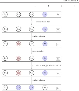
The general idea of the progress of the network of oscillators is visualised in Fig. 1. In the figure, each rounded rectangle shows a state of a network of four oscillators. The circles represents the nodes, where we inscribe its current phase and an abbreviation of its mode. A node that is about to fire is indicated by a starred circle, while a shaded circle indicates a node that is within the refractory period. The rectangle denotes the environment counter, with its corresponding value and mode. The phase response function is arbitrarily chosen, and of minor importance for the example.
In the first state, all outgoing transitions only check whether to increase the counter. Since no oscillator is in the firing phase, all oscillators just update their mode (observe that the single arrow actually denotes four transitions). In the next step, all oscillators increase their phase by one, and reset their mode tostart. In the next four transitions, oscillator 2 fires and increases the counter, which in turn is sufficient for oscillator 3 to fire as well. Hence they both increased the counter by one, while oscillators 1 and 4 did not. During the last transition of the example, oscillator 2 and 3 reset their phase to one, while oscillator 1 is perturbed and increases its phase by two steps at once. Oscillator 4 is within its refractory period, which means that it is not perturbed, and simply increments its phase. In addition to these transitions, we also need some bookkeeping transitions, to ensure that the counter is reset before the oscillators check their phase response. Furthermore, observe that in the example, it is crucial that oscillator 3 checks its response after oscillator 2 increased the counter, since otherwise 3 would not have been perturbed to fire.
of the current phase Φ of the oscillator and the mode θ within this phase. The phase ranges from 1 toT, while the mode takes values from{start,update}. Fur-thermore, we use a single counter to keep track of the number of oscillators that fired successfully within a single phase computation.
For a fixed sequence ofN oscillators, a state of the concrete model consists of a functionν that associates a phase and mode with each oscillator,
ν:{1, . . . , N} →({1, . . . , T} × {start,update}),
and the state of the environmentηthat counts the number of oscillators that fired, η∈ {start,update} × {0, . . . , N}.
A state is therefore a tuples= (η, ν), whereηis the state of the environment, and ν is the state of the network. We denote the set of all concrete system states by Qc. For simplicity, we use the notationpφ (pθ, respectively) for the corresponding
projection function of the network states, i.e., ifν(u) = (Φu, θu), thenpφ(ν(u)) =
Φu andpθ(ν(u)) =θu. Similarly, for an environment stateη= (θ, c), we will refer
to θ by pθ(η) and to cby pc(η). We use the notationinitΦ(s) = {u|pθ(ν(u)) = start∧pφ(ν(u)) =Φ}for the set of all oscillators sharing phaseΦ and modestart
in the state s = (η, ν). Furthermore, we simply use the notation init(s) = {u |
pθ(ν(u)) =start}.
We now define the transition probabilities between states. To do this we first distinguish the following cases:
1. the environment resets its counter; 2. no oscillator has a clock value ofT;
3. an oscillator is in the modestart, has a clock value lower thanT, is perturbed, but not enough to fire;
4. an oscillator is in the modestart, has a clock value lower than T and is per-turbed enough to fire;
5. an oscillator is in the modestart, has a clock value of T, and broadcasts its pulse;
6. an oscillator is in the modestart, has a clock value ofT, and fails to broadcast its pulse;
7. all oscillators are in the modeupdate, update their clock and reset their state tostart.
We will impose an order on certain transitions for two reasons. Firstly, we will restrict transitions that are only used for bookkeeping purposes. For example, we will require that the reset transition of the environment is taken before any of the transitions for the oscillators within a phase are activated. In particular, this means that each computation starts with a transition of the type 1. Secondly, we need to ensure that, if at least one oscillator fires, the phase response of all oscillators is evaluated starting with oscillators in the highest phase, down to the lowest phase, as described above. The cases stated above are reflected in the following definitions for the transition probability between two statess= (η, ν) ands′= (η′, ν′).
3,s 8,s 5,s 1,s 0,u
1 2 3 4
3,u 8,u 5,u 1,u 0,u
4,s 9,s 6,s 2,s 0,s
4,s 9,s 6,s 2,s 0,u
4,u 9,u 6,u 2,u 2,u
6,s 1,s 1,s 3,s 2,s
. . . check if osc. fire
. . . osc. 2 fires, perturbs 3 to fire update phases
reset counter
[image:10.595.80.418.70.460.2]update phases
Fig. 1: Transitions in the Concrete Oscillator Model (N= 4, T = 9, R= 2)
changes toupdateins′, and its value is set to 0. Since this transition is mandatory at the beginning of each round, its probability is 1.
Ifpθ(η) =start∧pθ(η′) =update∧pc(η′) = 0∧ ∀u:ν(u) =ν′(u), (1)
thenP(s, s′) = 1.
T at states. Hence we have to normalise the tranistion probability accordingly. Similarly, the probability of failing to fire is |initTµ(s)|.
Ifpθ(η) =updateand there is aws.t. (2)
pθ(ν(w)) =start∧pφ(ν(w)) =T∧pθ(ν′(w)) =update ∧pφ(ν(w)) =pφ(ν′(w))∧ ∀u:u6=w→ν(u) =ν′(u) ∧pc(η′) =pc(η) + 1
thenP(s, s′) = 1−µ
|initT(s)|
.
Ifpθ(η) =updateand there is aws.t. (3)
pθ(ν(w)) =start∧pφ(ν(w)) =T∧pθ(ν′(w)) =update ∧pφ(ν(w)) =pφ(ν′(w))∧ ∀u:u6=w→ν(u) =ν′(u) ∧pc(η′) =pc(η)
thenP(s, s′) = µ
|initT(s)|
.
If no oscillator is at the end of its cycle, that is, in case 2, we define the probability of one oscillator updating its mode as follows. Observe that we have to normalise the transition probability by the number of all oscillators that have not transitioned to their update mode yet. This is correct, since no oscillator fires, which also means that no oscillator can be activated beyond the maximum phase. This implies in particular that the order of oscillator transitions does not matter in this round.
Ifpθ(η) =update and there is aws.t. (4)
pθ(ν(w)) =start∧pθ(ν′(w)) =update∧pφ(ν(w)) =pφ(ν′(w)) ∧ ∀u:pφ(ν(u))< T∧ ∀u:u6=w→ν(u) =ν′(u)∧η=η′
then P(s, s′) = 1
|init(s)|.
Now we will consider the cases 3 and 4, where some oscillator already fired (i.e.,pc(η)>0), and other oscillators are perturbed. We distinguish between two
Ifpθ(η) =update and there is aws.t. (5)
pθ(ν(w)) =start∧pθ(ν′(w)) =update∧pφ(ν(w)) =pφ(ν′(w)) ∧pφ(ν(w))< T∧ ∃u:pφ(ν(u)) =T
∧ ∀u:u6=w→(pθ(ν(u)) =update∨pφ(ν(u))6pφ(ν(w))) ∧pφ(ν(w)) +∆(pφ(ν(w)), pc(η), ǫ) + 16T
∧ ∀u:u6=w→ν(u) =ν′(u)
∧η′=η
then P(s, s′) = 1
|initpφ(s(w))(s)|
.
The cases where a perturbed oscillator fires are analogous to oscillators with a maximal phase, except for the addititional conditions that some other oscillator fired, and that all oscillators with higher phases have already been considered.
Ifpθ(η) =update and there is aws.t. (6)
pθ(ν(w)) =start∧pθ(ν′(w)) =update∧pφ(ν(w)) =pφ(ν′(w)) ∧pφ(ν(w))< T∧ ∃u:pφ(ν(u)) =T
∧ ∀u:u6=w→(pθ(ν(u)) =update∨pφ(ν(u))6pφ(ν(w))) ∧pφ(ν(w)) +∆(pφ(ν(w)), pc(η), ǫ) + 1> T
∧ ∀u:u6=w→ν(u) =ν′(u)
∧η′=η
then P(s, s′) = µ
|initpφ(s(w))(s)|
Ifpθ(η) =update and there is aws.t. (7)
pθ(ν(w)) =start∧pθ(ν′(w)) =update∧pφ(ν(w)) =pφ(ν′(w)) ∧pφ(ν(w))< T∧ ∃u:pφ(ν(u)) =T
∧ ∀u:u6=w→(pθ(ν(u)) =update∨pφ(ν(u))6pφ(ν(w))) ∧pφ(ν(w)) +∆(pφ(ν(w)), pc(η), ǫ) + 1> T
∧ ∀u:u6=w→ν(u) =ν′(u)
∧pc(η′) =pc(η) + 1 ∧pθ(η′) =pθ(η)
then P(s, s′) = 1−µ
|initpφ(s(w))(s)|.
their mode tostart after the transition.
Ifpθ(η) =updateandpθ(η′) =start and (8)
for alluwe havepθ(ν(u)) =update∧pθ(ν′(u)) =start∧Fupdate
thenP(s, s′) = 1.
The formulaFupdate is an abbreviation for the conjunction of the following four
conditions, which model the update of the phases of the oscillators, according to the phase response function. Observe that the phases of the oscillators had not been updated by the previously defined transitions. Hence, we now update the phases of all oscillators at once.
∀u:pφ(ν(u)) =T → (8a)
pφ(ν′(u)) = 1
∀u:pφ(ν(u))< T∧pφ(ν(u))6R→ (8b)
pφ(ν′(u)) =pφ(ν(u)) + 1
∀u:pφ(ν(u))< T∧pφ(ν(u))> R∧ (8c)
pφ(ν(u)) +∆(pφ(ν(u)), pc(η), ǫ) + 16T →
pφ(ν′(u)) =pφ(ν(u)) +∆(pφ(ν(u)), pc(η), ǫ) + 1
∀u:pφ(ν(u))< T∧pφ(ν(u))> R∧ (8d)
pφ(ν(u)) +∆(pφ(ν(u)), pc(η), ǫ) + 1> T→
pφ(ν′(u)) = 1.
In this formula, (8a) handles the simple case of firing oscillators, while (8b) defines the behaviour of oscillators within their refractory period. The formulas (8c) and (8d) reflect the two cases where oscillators are perturbed, either not exceeding their oscillation cycle, or firing, respectively.
With this model, we could begin to analyse the synchronisation behaviour with respect to different phase response functions or broadcast failure probabilities. However, the state space of the model increases exponentially with the number of oscillators, which makes an analysis beyond small numbers of infeasible. To overcome this restriction, we increase the level of abstraction as presented in the next section.
5 Population Model
In this section, we define apopulation model of a network of pulse-coupled oscil-lators for parameters as defined in Sect. 4.1 asS = (∆, N, T, R, ǫ, µ). Oscillators in our model have identical dynamics, and two oscillators are indistinguishable if they share the same phase. That is, we can reason about groups of oscillators, instead of individuals. We therefore encode the global state of the model as a tu-plehk1, . . . , kTi where eachkΦ is the number of oscillators sharing a phase value
σ0 kk11 σ0 k2 σ0 2 σ0 1 σ0 σ0 σ0 5 σ0 σ0
σ0 σσ11 kk11
k2 σ1 σ1 2 σ1 1 σ1 σ1 σ1 5 σ1
σ1 σσ22 kk11
k2 σ2 σ2 σ2 2 σ2 1 σσσ222
5
σ2 σσ33 kk11
k2
σ3
σ3
σ3
σ3
2 σ3
1
σ3
σ3
σ3
[image:14.595.71.421.73.163.2]5
Fig. 2: Evolution of the global state over four discrete time steps.
Definition 6 A global state of a population model S = (∆, N, T, R, ǫ, µ) is a T -tupleσ ∈ {0, . . . , N}T, where σ= hk1, . . . , kTi andPTΦ=1kΦ = N. The set of all
global states ofS isΓ(S), or simplyΓ whenS is clear from the context.
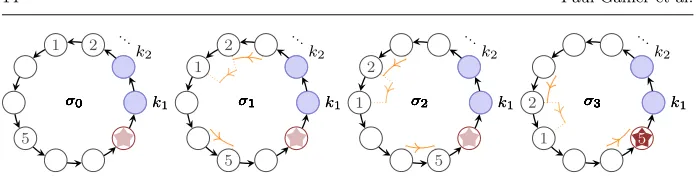
Example 1 Figure 2 shows four global states for an instantiated population model ofN = 8 oscillators with T = 10 discrete values for their phase and a refractory period of length R = 2. We assume that the phase response function is linear, that is, ∆(Φ, α, ǫ) = [Φ·α·ǫ], where [·] denotes rounding to the closest integer. Furthermore, letǫ= 0.115. For exampleσ0=h0,0,2,1,0,0,5,0,0,0iis the global
state where two oscillators have a phase of three, one oscillator has a phase of four, and five oscillators have a phase of seven. The starred node indicates the number of oscillators with phase ten that will fire in the next moment in time, while the shaded nodes indicate oscillators with phases that lie within the refractory period (one and two). If no oscillators have some phaseΦ then we omit the 0 in the corresponding node. Observe that, while going from σi−1 to σi (1 6i63),
the oscillator phases increase by one. In the next section, we will explain how transitions between these global states are made. Note that directional arrows indicate cyclic direction, and do not represent transitions.
With every stateσ∈Γ we associate a non-empty set offailure vectors, where each failure vector is a tuple of broadcast failures that could occur inσ.
Definition 7 Afailure vector is a T-tupleF =hf1, . . . , fTi ∈({0, . . . , N} ∪ {⋆})T,
where fi = ⋆ implies fj = ⋆ for all 16j 6 i. We denote the set of all possible
failure vectors byF.
Given a failure vector F =hf1, . . . , fTi, fΦ ∈ {0, . . . , N} indicates the number of
broadcast failures that occur for all oscillators with a phase of Φ. If fΦ =⋆then
no oscillators with a phase ofΦfire. Semantically,fΦ= 0 andfΦ=⋆differ in that
the former indicates that all (if any) oscillators with phaseΦfire and no broadcast failures occur, while the latter indicates that all (if any) oscillators with a phase ofΦdo not fire. If no oscillators fire at all in a global state then we have only one possible failure vector, namely{⋆}T.
5.1 Transitions
Absorptions. For real deployments of synchronisation protocols it is often the case that the duration of a single oscillation cycle will be at least several seconds [10, 28]. The perturbation induced by the firing of a group of oscillators may lead to groups of other oscillators to which they are coupled firing in turn. The firing of these other oscillators may then cause further oscillators to fire, and so forth, leading to a “chain reaction”, where each group of oscillators triggered to fire isabsorbed by the initial group of firing oscillators. Since the whole chain reaction of absorptions may occur within just a few milliseconds, and in our model the oscillation cycle is a sequence of discrete states, when a chain reaction occurs the phases of all perturbed oscillators are updated at one single time step.
Since we are considering a fully connected network of oscillators, two oscillators sharing the same phase will have their phase updated to the same value in the next time step. They will always perceive the same number of other oscillators firing. Therefore, for each phaseΦwe define the functionαΦ:Γ× F → {0, . . . , N}, where αΦ(σ, F) is the number of oscillators with a phase greater thanΦperceived to be firing by oscillators with phaseΦ, in some global state, incorporating the broadcast failures defined in the failure vectorF. This allows us to encode the aforementioned chain reactions of firing oscillators. Note that our encoding of chain reactions results in a global semantics that differs from typical parallelisation operations, for example, the construction of the cross product of the individual oscillators. Observe that, in the concrete model of Sect. 4.2, we modelled such a behaviour by case 4.
Given a global state σ = hk1, . . . , kTi and a failure vector F = hf1, . . . , fTi,
the following mutually recursive definitions show how we calculate the values α1(σ, F), . . . , αT(σ, F), and how functions introduced in Sect. 4.1 are modified to
indicate the update in phase, and firing, ofall oscillators sharing the same phase Φ. Observe that to calculate any αΦ(σ, F) we only refer to definitions for phases greater thanΦ and the base case is Φ=T, that is, values are computed from T down to 1. The function ref is the refractory function as defined in Sect. 4.1.
updateΦ(σ, F) = 1 + ref(Φ, ∆(Φ, αΦ(σ, F), ǫ)) (9)
fireΦ(σ, F) =updateΦ(σ, F)> T (10)
αΦ(σ, F) =
0 ifΦ=T
αΦ+1(σ,F)+kΦ+1−fΦ+1 ifΦ<T, fΦ+16=⋆ andfireΦ+1(σ,F)
αΦ+1(σ, F) otherwise
(11)
Transition Function. We now define the transition function that maps phase val-ues to their updated valval-ues in the next time step. Note that since we no longer distinguish different oscillators with the same phase we only need to calculate a single value for their evolution and perturbation.
Definition 8 The phase transition function τ : Γ × {1, . . . , T} × F → N maps a global stateσ, a phaseΦ, and some possible failure vectorF forσ, to the updated phase in the next discrete time step, with respect to the broadcast failures defined inF, and is defined as
τ(σ, Φ, F) =
(
1 iffireΦ(σ, F)
LetUΦ(σ, F) be the set of phase valuesΨ where all oscillators with phaseΨ in
σ will have their phase updated toΦ in the next time step, with respect to the broadcast failures defined inF. Formally,
UΦ(σ, F) ={Ψ |Ψ∈ {1, . . . , T} ∧τ(σ, Ψ, F) =Φ}. (13)
We can now calculate the successor state of a global stateσ and define how the model evolves over time.
Definition 9 Thesuccessor functionsucc :→ Γ× F →Γ maps a global stateσand a failure vectorF to a stateσ′, and is defined assucc(→ hk1, . . . , kTi, F) =hk′1, . . . , k′Ti,
wherekΦ′=P
Ψ∈UΦ(σ,F)kΨ for 16Φ6T.
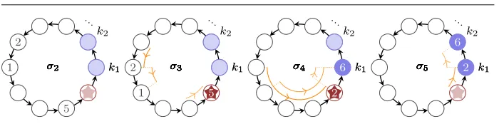
Example 2 Recall that the perturbation function of our example was given as ∆(Φ, α, ǫ) = [Φ·α·ǫ], where [·] denotes rounding and ǫ = 0.115. Consider the global stateσ2 of Fig 3 where no oscillators will fire sincek10 = 0. We therefore
have one possible failure vector forσ0, namelyF={⋆}10. Since no oscillators fire
the dynamics of the oscillators are determined solely by their standalone evolu-tion, and all oscillators simply increase their phase by 1 in the next time step. Now consider the global stateσ3andF=h⋆, ⋆, ⋆, ⋆, ⋆, ⋆,1,0,0,0i, a possible failure
vector for σ3, indicating that oscillators with phases of 7 to 10 will fire and one
broadcast failure will occur for the single oscillator that will fire with phase 7. Here a chain reaction occurs as the perturbation induced by the firing of the 5 oscillators causes the single oscillator with a phase of 7 to also fire. A broadcast failure occurs when this single oscillator fires, and the perturbation of the 5 firing oscillators is insufficient to cause the 2 oscillators with a phase of 6 to also fire. In the next state the oscillator with phase 7 has been absorbed by the group of the 5 oscillators that had phase 10.
More explicitly, sincefire10(σ3, F) holds we have thatα9(σ3, F) =α10(σ3, F) +
k10−f10= 0+5−0 = 5. Now, since∆(9,5,0.14) = [9·5·0.115] = [5.175] = 5, we have update9(σ3, F) = 15>10, and thus,fire9 holds. Hence, we have thatα8(σ3, F) =
α9(σ3, F) +k9−f9 = 0 + 5−0 = 5, and similarly, due to∆(8,5,0.115) = 5,fire8
holds. That is, we have thatα7(σ3, F) =α8(σ3, F) +k8−f8= 0 + 5−0 = 5. We
then continue calculatingαΦ(σ3, F) for 6>Φ>1, and noting that∆(6,5,0.115) =
[3.45] = 3. Hencefire6(σ3, F) does not hold, and we obtainα1(σ3, F) =α2(σ3, F) =
α3(σ3, F) =α4(σ3, F) =α5(σ3, F) =α6(σ3, F) =α7(σ3, F) = 5. We conclude that U1(σ3, F) ={10,9,8,7},U10(σ3, F) ={6,5},U9(σ3, F) ={4,3}, andUΦ(σ3, F) =∅
for 9> Φ >3. SinceR= 2 we have thatU3(σ3, F) ={2}andU2(σ3, F) ={1}. We
calculate the successor ofσ3 asσ4=
→
succ(h⋆, ⋆, ⋆, ⋆, ⋆, ⋆,1,0,0,0i, F) =hk10+k9+
k8+k7, k1, k2,0,0,0,0,0, k4+k3, k6+k5i=h6,0,0,0,0,0,0,0,0,2i.
Lemma 1 The number of oscillators is invariant during transitions, i.e., the succes-sor function only creates tuples that are states of the given model. Formally, let σ=
hk1, . . . , kTiandσ′=hk1′, . . . , k′Tibe two states of a modelSsuch thatσ′ =
→ succ(σ, F), whereF is some possible failure vector forσ. ThenPT
σ2 kk11 σ2 k2 σ2 σ2 σ2 2 σ2 1 σσσ222
5
σ2 σσ33 kk11
k2
σ3
σ3
σ3
σ3
2 σ3
1
σ3
σ3
σ3
5
σ4 6 kk11
σ4 k2 σ4 σ4 σ4 σ4 σ4 σ4 σ4 σ4 2
σ5 2 kk11
[image:17.595.71.421.77.164.2]σ5 6 k2 σ5 σ5 σ5 σ5 σ5 σ5 σ5 σ5
Fig. 3: Evolution of the global state over four discrete time steps.
Φ∈ {1, . . . , T}, we have that 16τ(σ, Φ, F)6T. Hence for all Ψ with 16Ψ 6T, there is a Φ such that Ψ ∈ UΦ(σ, F). This implies STΦ=1UΦ(σ, F) = {1, . . . , T}.
Furthermore, there cannot be more than oneΦsuch thatΨ ∈ UΦ(σ, F), sinceτ is
functional. Now we havePT Φ=1k
′
Φ= PT
Φ=1
P
Ψ∈UΦ(σ,F)kΨ = PT
Φ=1kΦ=N. ⊓⊔
5.2 Failure Vector Calculation
We construct all possible failure vectors for a global state by considering every group of oscillators in decreasing order of phase. At each stage we determine if the oscillators would fire. If they fire then we consider each outcome where any, all, or none of the firings result in a broadcast failure. We then add a corresponding value to a partially calculated failure vector and consider the next group of oscillators with a lower phase. If the oscillators do not fire then there is nothing left to do, since by Def. 4 we know that∆is increasing, therefore all oscillators with a lower phase will also not fire. We can then pad the partial failure vector with ⋆ appropriately to indicate that no failure could happen since no oscillator fired.
Table 1 illustrates how a possible failure vector for global stateσ3 in Fig. 3 is
iteratively constructed. The first three columns respectively indicate the current iterationi, the global stateσ3with the currently considered oscillators underlined,
and the elements of the failure vectorFcomputed so far. The fourth column istrue
if the oscillators with phaseT+1−iwould fire given the broadcast failures in the partial failure vector. We must consider all outcomes of any or all firings resulting in broadcast failure. The final column therefore indicates whether the value added to the partial failure vector in the current iteration is the only possible value (false), or a choice from one of several possible values (true).
[image:17.595.84.403.584.652.2]Initially we have an empty partial failure vector. At the first iteration there are 5 oscillators with a phase of 10. These oscillators will fire so we must consider each
Table 1: Construction of a possible failure vector for a global state σ3 = h0,0,0,0,0,2,1,0,0,5i.
case where 0,1,2,3,4 or 5 broadcast failures occur. Here we choose 0 broadcast failures, which is then added to the partial failure vector. At iterations 2 and 3 the oscillators would have fired, but since there are no oscillators with a phase of 9 or 8 we only have one possible value to add to the partial failure vector, namely 0. At iteration 4 a single oscillator with a phase of 7 fires, and we choose the case where the firing resulted in a broadcast failure. In the final iteration oscillators with a phase of 6 do not fire, hence we can conclude that oscillators with phases less than 6 also do not fire, and can fill the partial failure vector appropriately with⋆.
Formally, we define a family of functionsfail indexed by Φ, where eachfailΦ
takes as parameters some global state σ, and V, a vector of length T −Φ. V represents all broadcast failures for all oscillators with a phase greater than Φ. The functionfailΦ then computes the set of all possible failure vectors forσwith suffixV. Here we use the notationv⌢v′ to indicate vector concatenation. Definition 10 We definefailΦ :Γ × {0, . . . , N}T−Φ →P(({0, . . . , N} ∪ {⋆})T), for 16Φ6T, as the family of functions indexed byΦ, where σ=hk1, . . . , kTiand
failΦ(σ, V) =
SkΦ
k=0failΦ−1(σ,hki⌢V) if 1< Φ6T andfireΦ(σ,{⋆}Φ⌢V)
Sk1 k=0{hki
⌢V} ifΦ= 1 andfire1(σ,h⋆i⌢V) n
{⋆}Φ⌢Vo otherwise
Observe that the result offailT is always a set of well defined failure vectors, since whenever⋆is introduced into a failure vector at indexΦ, all preceding indices are also filled with⋆, as required by Definition 7.
Definition 11 Given a global state σ ∈ Γ, we define Fσ, the set of all possible
failure vectors for that state, asFσ=failT(σ,hi), and definenext(σ), the set of all
successor states ofσ, asnext(σ) ={succ(σ, F)→ |F ∈ Fσ}.
Note that for some global states|next(σ)|<|Fσ|, since we may have that
→
succ(σ, F) = →
succ(σ, F′) for someF, F′∈ Fσ withF6=F′.
Given a global stateσ and a failure vectorF ∈ Fσ, we will now compute the
probability of a transition being made to state succ(σ, F→ ) in the next time step. Recall thatµ is the probability with which a broadcast failure occurs. Firstly we define the probability mass functionPMF:{1, . . . , N}2 →[0,1], wherePMF(k, f) gives the probability off broadcast failures occurring given thatkoscillators fire, as PMF(k, f) =µf(1−µ)k−f(k
f). We then denote by PFV : Γ × Fσ →[0,1] the
function mapping a possible broadcast failure vectorF forσ, to the probability of the failures inF occurring. That is,
PFV(hk1, . . . , kTi,hf1, . . . , fTi) = T Y
Φ=1
(
PMF(kΦ, fΦ) iffΦ6=⋆
1 otherwise (14)
Lemma 2 For any global state σ, PFVis a discrete probability distribution overFσ. Formally,P
Proof Given a global state σ = hk1, . . . , kTi we can construct a tree of depth T
where each leaf node is labelled with a possible failure vector forσ, and each node Λ at depth Φ is labelled with a vector of length Φ corresponding to the last Φ elements of a possible failure vector for σ. We denote the label of a nodeΛ by V(Λ). We label each nodeΛω withhωi⌢V(Λ). We iteratively construct the tree,
starting with the root node,root, at depth 0, which we label with the empty tuple
hi. For each nodeΛat depth 06Φ < T we construct the children ofΛas follows: 1. If oscillators with phaseΦfire we define the sample space Ω={0, . . . , nΦ} to
be a set of disjoint events, where eachω∈Ω is the event whereω broadcast failures occur, given thatkΦoscillators fired. For eachω∈Ωthere is a childΛω
ofΛwith labelhωi⌢V(Λ), and we label the edge fromΛtoΛ
ωwithPMF(kΦ, ω).
2. If oscillators with phaseΦdo not fire thenΛhas a single childΛ⋆labelled with h⋆i⌢V(Λ), and we label the edge fromΛtoΛ⋆with 1.
We denote the label of an edge from a node Λ to its child Λ′ by L(Λ, Λ′). For case 2 we can observe that if oscillators with phase Φ do not fire then we know that oscillators with any phaseΨ < Φwill also not fire, since from Def. 4 we know that∆is an increasing function. Hence, all descendants ofΛwill also have a single child, with an edge labelled with 1, and each node is labelled with the label of its parent, prefixed withh⋆i.
After constructing the tree we have a vector of lengthT associated with each leaf node, corresponding to a failure vector forσ. The setFσof all possible failure
vectors for σis therefore the set of all vectors labelling leaf nodes. We denote by
P↓(Λ) the product of all labels on edges along the path fromΛback to the root. Given a global state σ= hk1, . . . , kTi and a failure vectorF = hf1, . . . , fTi ∈ Fσ
labelling some leaf nodeΛat depthT, we can see that
P↓(Λ) = 1· T Y
Φ=1
(
PMF(kΦ, fΦ) iffφ6=⋆
1 otherwise =PFV(σ, F).
LetDΦ denote the set of all nodes at depthΦ. We showP
d∈DΦP↓(d) = 1 by
induction onΦ. ForΦ= 0, i.e.,DΦ={root}, the property holds by definition. Now assume thatP
d∈DΦP↓(d) = 1 holds for some 06Φ < T. Let Λbe some node in
DΦ, and letCΛbe the set of all children ofΛ. Consider the following two cases: If oscillators with phaseΦdo not fire then|CΛ|= 1, and for the onlyc∈CΛwe have thatL(Λ, c) = 1. If oscillators with phaseΦfire observe thatPMFis a probability mass function for a random variable defined on the sample spaceΩ={0, . . . , kΦ}.
In either case we can see thatP
c∈CΛL(Λ, c) = 1. Note thatDΦ+1 = S
d∈DΦCd,
and recall thatL(d, c)·P↓(d) =P↓(c). Therefore,
X
d∈DΦ+1
P↓(d) = X
d∈DΦ X
c∈Cd
L(d, c)·P↓(d) = X
d∈DΦ
P↓(d) X
c∈Cd
L(d, c)
.
Since P
c∈CdL(d, c) = 1 for eachd∈DΦ, and from the induction hypothesis, we
then have that
X
d∈DΦ
P
↓(d) X c∈Cd
L(d, c)
=
X
d∈DΦ
We have already shown thatP↓(Λ) =PFV(σ, F) for any leaf nodeΛlabelled with a failure vectorF, and since the set of all labels for leaf nodes isFσ we can conclude
that
X
F∈Fσ
PFV(σ, F) = X
d∈DT
P↓(d) = 1.
This proves the lemma. ⊓⊔
Example 3 We consider again the global states σ3 = h0,0,0,0,0,2,1,0,0,5i and
σ4=h6,0,0,0,0,0,0,0,0,2i, given in Fig. 3, of the population model instantiated
in Example 1, and the failure vectorF=h⋆, ⋆, ⋆, ⋆, ⋆, ⋆,1,0,0,0igiven in Example 2, noting thatF ∈ Fσ3,
→
succ(σ3, F) =σ4, andµ= 0.1. We calculate the probability
of a transition being made fromσ3 toσ4 as
PFV(h0,0,0,0,0,2,1,0,0,5i,h⋆, ⋆, ⋆, ⋆, ⋆, ⋆,1,0,0,0i)
= 1·1·1·1·1·1·PMF(1,1)·PMF(0,0)·PMF(0,0)·PMF(5,0) = (0.11·0.90·1)·(1)·(1)·(0.10·0.95·1) = 0.059049
We now have everything we need to fully describe the evolution of the global state of a population model over time. An execution path of a population model
S is an infinite sequence of global statesω=σ0σ1σ2σ3· · ·, whereσ0 is called the initial state, andσk+1 ∈next(σ) for allk>0.
5.3 Synchronisation
When all oscillators in a population model have the same phase in a global state we say that the state is synchronised. Formally, a global stateσ=hk1, . . . , kTi is synchronised if, and only if, there is some Φ∈ {1, . . . , T} such thatkΦ = N, and
hencekΦ′ = 0 for all Φ′ 6=Φ. We will often want to reason about whether some particular run ωof a model leads to a global state that is synchronised. We say that a pathω=σ0σ1· · · synchronises if, and only if, there exists somek>0 such
thatσk is synchronised. Once a synchronised global state is reached any successor
states will also be synchronised. Finally we can say that a model synchronises if, and only if, all runs of the model synchronise.
5.4 Model Construction
Given a population model S = (∆, N, T, R, ǫ, µ) we construct a DTMC D(S) = (Q, σ0,P, L) whereLranges over the singleton{synch}. We define the set of states
Q to be Γ(S)∪ {σ0}, where σ0 is the initial state of the DTMC. For each σ = hk1, . . . , kTi ∈Γ(S), we setL(σ) ={synch}ifkT =N.
In the initial state all oscillators areunconfigured. That is, oscillators have not yet been assigned a value for their phase. For eachσ=hk1, . . . , kTi ∈Q\ {σ0}we
define
P(σ0, σ) = 1
TN
N k1, . . . , kT
to be the probability of moving fromσ0to a state wherekiarbitrary oscillators are
configured with the phase valueifor 16i6T. The multinomial coefficient defines the number of possible assignments of phases to distinct oscillators that result in the global stateσ. The fractional coefficient normalises the multinomial coefficient with respect to the total number of possible assignments of phases to all oscillators. In general, given an arbitrary set of initial configurations (global states) for the oscillators, the total number of possible phase assignments can be calculated by computing the sum of the multinomial coefficients for each configuration (global state) in that set. SinceΓ is the set of all possible global states, we have that
X
hk1,...,kTi∈Γ
N k1, . . . , kT
!
=TN.
We assign probabilities to the transitions as follows: for everyσ∈Q\ {σ0}, we consider eachF∈ Fσ, and setP(σ,succ(σ, F→ )) =PFV(σ, F). For every combination
ofσandσ′ whereσ′6∈next(σ) we setP(σ, σ′) = 0.
5.5 Model Reduction
We now describe a reduction of the population model that results in a significant decrease in the size of the model, but is equivalent to the original model with re-spect to the reachability of synchronised states. We first distinguish between states where one or more oscillators are about to fire, and states where no oscillators will fire at all. We refer to these states asfiring statesandnon-firingstates respectively.
Definition 12 Given a population modelS, a global state hk1, . . . , kTi ∈ Γ is a firing state if, and only if, kT >0. We denote byΓF the set of all firing states of S, and denote byΓNF=Γ \ΓFthe set of all non-firing states of S. We will again omitS if it is clear from the context
Given a DTMCD= (Q, σ0,P, L) let|P|=|{(t, t′)|t, t′∈Q2andP(t, t′)>0}|
be the number of non-zero transitions in P, and |D| =|Q|+|P| to be the total number of states and non-zero transitions inD.
Theorem 1 For every population model S and its corresponding DTMC D(S) = (Q, σ0,P, L), there is a reduced modelD′(S) = (Q′, σ0,P′, L′)where|D′(S)|<|D(S)| and unbounded-time reachability properties with respect to synchronised firing states in
D(S) are preserved in D′(S). In particular, the states and transitions in D(S) are reduced inD′(S)such that Q′=Q\ΓNF and
|Q′|= 1 + T
(N−1)
(N−1)!,
|P′|6|P| −2|ΓNF| wherex(n)is the rising factorial.
Lemma 3 Every non-firing stateσ∈ΓNFhas exactly one successor state, and in that state all oscillator phases have increased by1.
Proof Given a non-firing state σ = hk1, . . . , kTi observe that as kT = 0 there is
only one possible failure vector forσ, namely{⋆}T. The set of all successor states ofσ is then the singleton {succ(σ,→ {⋆}T)}. By construction we can then see that updateΦ(σ,{⋆}T) = 1 andUΦ(σ,{⋆}T) ={Φ−1}for 16Φ6T. The single successor
state is then given bysucc(σ,→ {⋆}T) =h0, k
1, . . . , kT−1i. ⊓⊔
Corollary 1 An immediate corollary of Lemma 3 is that a transition from any non-firing state is taken deterministically, since for anyσ∈ΓNFwe havePFV(σ,{⋆}T) = 1. Reachable State Reduction. Given a path ω = σ0· · ·σn−1σn where σi ∈ ΓNF for
0 < i < n and σ0, σn ∈ ΓF, we omit transitions (σi, σi+1) for 0 6 i < n, and
instead introduce a direct transition fromσ0, the first firing state, toσn, the next
firing state in the sequence. For anyσ=hk1, . . . , kTi ∈Γ let δσ = max{Φ|kΦ >
0 and 16Φ6T}be the highest phase of any oscillator inσ. The successor state of a non-firing state is then the state where all phases have increased by T−δσ.
Observe thatT−δσ= 0 for any σ∈ΓF.
Definition 13 Thedeterministic successor functionsucc :։ Γ →ΓF, given by
։
succ(hk1, . . . , kTi) ={0}T−δσ ⌢
hk1, . . . , kδσi,
maps a stateσ∈Γ to the next firing state reachable by takingT−δσdeterministic
transitions. Observe that for any firing stateσ we have δσ =T, and hence that
։
succ(σ) =σ.
We now update the definition for the set of all successor states for some global stateσ∈Γ to incorporate the deterministic successor function.
Definition 14 Given a global stateσ ∈Γ, we define next։ (σ) to be the set of all successor states ofσ, where
։
next(σ) ={succ(։ succ(σ, F))→ |F ∈ Fσ}.
Definition 15 Given a firing stateσ∈ΓFlet pred(σ) be the set of all non-firing predecessors ofσ, whereσis reachable from the predecessor by taking some positive number of transitions deterministically. Formally,
pred(σ) ={σ′|σ′∈ΓNFandsucc(σ։ ′) =σ}. We refer to all statesσ′∈pred(σ) as deterministic predecessors ofσ.
Then givenD= (Q, σ0,P, L) withQ={σ0} ∪Γ, we defineQ′=Q\Sσ∈ΓFpred(σ) to be the reduction ofQwhere all non-firing states from which a firing state can be reached deterministically are removed.
σ0
σi =h1,1,0,0,0,0i
σi+1=h0,1,1,0,0,0i
σi+2=h0,0,1,1,0,0i
σi+3=h0,0,0,1,1,0i
σi+4=h0,0,0,0,1,1i P(σ0, σi)
P(σ0, σi+1)
P(σ0, σi+2)
P(σ0, σi+3)
P(σ0, σi+4)
P(σi, σi+1) = 1
P(σi+1, σi+2) = 1
P(σi+2, σi+3) = 1
[image:23.595.74.408.80.217.2]P(σi+3, σi+4) = 1
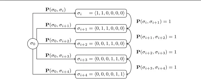
Fig. 4: Five possible initial configurations inQforN = 2,T = 6.
Proof Let P =S
σ∈ΓFpred(σ) be the set of all predecessors of firing states in ΓF. SinceQ=Γ∪ {σ0}andQ′=Q\P we can see thatQ′=ΓF∪ {σ0}if, and only if, P =ΓNF. From Definition 15 it follows thatP ⊆ΓNF. In addition, for anyσ∈ΓNF there is some stateσ′ such thatσ∈pred(σ′) andσ′=succ(σ)։ ∈ΓF, henceΓNF⊆P and the lemma is proved. ⊓⊔
Lemma 5 For a population modelS= (∆, N, T, R, ǫ, µ)and its corresponding DTMC
D = (Q, σ0,P, L) withQ= Γ ∪ {σ0}, the number of states in the reduction of Q is given by|Q′|= 1 +T(N−1)
(N−1)!,wherex
(n) is the rising factorial.
Proof Observe that there are (N+NT−1) ways to assignTdistinguishable phases toN indistinguishable oscillators [15]. SinceQ=Γ∪ {σ0}andΓ is the set of all possible configurations for oscillators we can see that|Q|= (N+NT−1) + 1. For any non-firing stateσ=hk1, . . . kTi ∈ΓNFwe know from Definition 6 that
PT
Φ=1kΦ=N and from
Definition 12 thatkT = 0, so it must be the case thatPTΦ−=11kΦ=N. That is, there
must be (N+NT−2) ways to assignT−1 distinguishable phases toNindistinguishable oscillators, and so|ΓNF|= (N+T−2
N ). From Lemma 4 we know thatQ
′=Q\ΓNFso it must be the case that|Q′|=|Q| − |ΓNF|= 1 + (N+T−1
N )−(N+T
−2
N ) = 1 +T (N−1)
(N−1)!. ⊓
⊔
Transition Matrix Reduction. Here we describe the reduction in the number of non-zero transitions in the model. We ilustrate how initial transitions to non-firing states are removed by using a simple example, and then describe how we remove transitions from firing states to any successor non-firing states..
Figure 4 shows five possible initial configurations σi, . . . , σi+4 ∈Q forN = 2
oscillators with T = 6 values for phase, where a transition is taken from σ0 to
each σk with probability P(σ0, σk). Any infinite run of D where a transition is
taken fromσ0 to one of the configured statesσi, . . . , σi+3 will pass throughσi+4,
since all transitions (σi+k, σi+k+1) for 06k63 are taken deterministically. Also,
observe that statesσi, . . . , σi+3are not inQ′, sinceσi+4is reachable from each by
σ0toσi+4 and each of its predecessors inP. Generally, given a stateσ∈Q′where
σ6=σ0, we setP′(σ0, σ) =P(σ0, σ) +Pσ′∈pred
(σ)P(σ0, σ
′).
We now define how we calculate the probability with which a transition is taken from a firing state to each of its possible successors. For each firing state σ∈Q′ we consider each possible successorσ′∈next։ (σ) of σand defineFσ→σ′ to be the set of all possible failure vectors for σ for which the successor ofσ is σ′, given by Fσ→σ′ = {F ∈ Fσ |
։
succ(succ(σ, F)) =→ σ′}. We then set the probability with which a transition fromσtoσ′ is taken toP′(σ, σ′) =P
F∈Fσ→σ′PFV(σ, F). Lemma 6 For a population model S = (∆, N, T, R, ǫ, µ), the corresponding DTMC
D= (Q, σ0,P, L)withQ={σ0} ∪Γ, and its reduction D′(S) = (Q′, σ0,P′, L′), the transitions inPare reduced inP′ such that|P′|6|P| −2|ΓNF|
Proof From Lemma 4 we know that|Q′|=|Q\ΓNF|, and hence that|ΓNF|transitions fromσ0 to non-firing states are not inP′, and from Lemma 3 we also know that
there is one transition from each non-firing state to its unique successor state that is not inP′. Since no additional transitions are introduced in the reduction it is clear that|P′|6|P| −2|ΓNF|. ⊓⊔
Lemma 7 For every population model DTMC D = (Q, σ0,P, L), unbounded-time reachability properties with respect to synchronised firing states in D are preserved in its reductionD′.
Proof We want to show that for every ⊲⊳ ∈ {<,6,>, >} and every λ ∈ [0,1], if σ0 |= P⊲⊳λ[Fsynch] holds in D then it also holds in D′. From the semantics of
PCTL over a DTMC we have
σ0|= P⊲⊳λ[Fsynch] ⇔ Pr{ω∈PathsD|ω|= Fsynch}⊲⊳ λ.
Therefore we need to show that
PrD{ω∈PathsD|ω|= Fsynch}=σPrD
′
{ω′∈PathsD
′
|ω′|= Fsynch}, wherePrD andPrD′ denote the probability measures with respect to the sets of infinite paths fromσ0inD andD′ respectively.
Given a firing stateσF∈Qwe denote byPathsD
σFthe set of all infinite paths ofD starting inσ0where the first firing state reached along that path isσF. All such sets
for all firing states inQform a partition, such thatS
σF∈ΓFPathsDσF=PathsD. That is, for all firing statesσF, σF′∈QwhereσF6=σF′we have thatPathsD
σF∩PathsDσF′=∅. Now observe that any infinite pathω of D can be written in the form ω = σ0ω1NFσF1ω2NFσ2F· · · where σiF is the ith firing state in the path and each ωNFi =
σ1iσi2· · ·σiki is a possibly empty sequence of ki non-firing states. Then for every
such path in D there is a corresponding pathω′ ofD′ without non-firing states, and of the form ω′ = σ0σF1σ2Fσ3F· · ·, as for any i we have σji ∈ pred(σiF) for all
16j6ki. As only deterministic transitions have been removed in D′ we can see thatPrD{σF
1ω2NFσ2F· · · } =PrD
′
{σF
1σ2FσF3· · · }. Hence, we only have to consider the
finite paths fromσ0 toσF1. To that end, observe that there are
pred(σF1)
possible
prefixes for each path fromσ0toσF1where the initial transition is taken fromσ0to
some non-firing predecessor ofσF
1, plus the single prefix where the initial transition
is taken toσF
1itself. Overall there are exactly
pred(σF1)
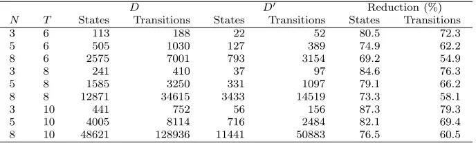
Table 2: Reduction in state space and transitions for different model instances.
D D′ Reduction (%)
N T States Transitions States Transitions States Transitions
3 6 113 188 22 52 80.5 72.3
5 6 505 1030 127 389 74.9 62.2
8 6 2575 7001 793 3154 69.2 54.9
3 8 241 410 37 97 84.6 76.3
5 8 1585 3250 331 1097 79.1 66.2
8 8 12871 34615 3433 14519 73.3 58.1
3 10 441 752 56 156 87.3 79.3
5 10 4005 8114 716 2484 82.1 69.4
8 10 48621 128936 11441 50883 76.5 60.5
that haveω′as their corresponding path inD′. We denote the set of these prefixes for a pathω′ inD′ byPref(ω′). Since the measure of each finite prefix extends to a measure over the set of infinite paths sharing that prefix, it is sufficient to show that the sum of the probabilities for these finite prefixes is equal to the probability of the unique prefixσ0, σF1ofω′, that isPrDPref(ω′) =PrD
′
{σ0, σ1}F . We can then
write
PrDPref(ω′) =P(σ0, σ1F) +
X
σ′∈pred
(σF
1)
P(σ0, σ′)·1kσ′
=P(σ0, σ1F) +
X
σ′∈pred
(σF
1)
P(σ0, σ′),
wherekσ′ is the number of deterministic transitions that lead fromσ′ toσF
1 inD.
Now recall that for anyσ∈Q′\ {σ0}we have P′(σ0, σ) =P(σ0, σ) +
X
σ′∈pred(σ)
P(σ0, σ).
So we have shown thatPrDPref(ω′) =PrD′{σ0, σF1}and the lemma is proved. ⊓⊔ Proof (of Theorem 1) Follows from Lemmas 5 and 6 for the reduction of states and transitions respectively, and from Lemma 7 for the preservation of unbounded time reachability properties.
5.6 Empirical Analysis
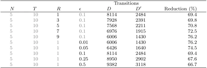
[image:25.595.137.355.321.376.2]Table 3: Reduction in transitions for different population model instances.
Transitions
N T R ǫ D D′ Reduction (%)
5 10 1 0.1 8114 2484 69.4
5 10 3 0.1 7928 2391 69.8
5 10 5 0.1 7568 2211 70.8
5 10 7 0.1 6976 1915 72.5
5 10 9 0.1 6006 1430 76.2
5 10 1 0.01 6006 1430 76.2
5 10 1 0.05 6426 1640 74.5
5 10 1 0.1 8114 2484 69.4
5 10 1 0.25 8950 2902 67.6
5 10 1 0.5 9382 3118 66.7
Table 3 shows the number of transitions of the DTMC, and corresponding re-duction, for various population model instances, and again uses the Mirollo and Strogatz model of synchronisation. Increasing the length of the refractory period (R) results in an increase in the reduction of transitions in the model. A longer re-fractory period leads to more firing states where the firing of a group of oscillators is ignored. This results in successor states having oscillators with lower values for phase, and hence a longer sequence of deterministic transitions (later removed in the reduction) leading to the next firing state. Conversely, increasing the strength of the coupling between oscillators (ǫ) results in a decrease in the reduction of transitions in the model. For the Mirollo and Strogatz model of synchronisation used here, increasing the coupling strength results in a linear increase in the per-tubation to phase induced by the firing of an oscillator. This results in successor states of firing states having oscillators with higher values for phase, and hence a shorter sequence of deterministic transitions leading to the next firing state.
5.7 Reward Structures for Reductions
While probabilistic reachability properties allow us to quantitatively analyse mod-els with respect to the likelihood of reaching a synchronised state, they do not allow us to reason about other properties of interest, for instance the expected time taken for the network to synchronise [16], or the expected energy consumption of the net-work [17]. Therefore, we will often want to augment the DTMC corresponding to a population model with rewards. We do this by annotating states and transitions with real-valued rewards (respectively costs, should values be negative) that are awarded when states are visited, or transitions taken.
For any finite pathω=σ0· · ·σk ofD we define the total reward accumulated
along that path up to, but not including,σk as
totR(σ0· · ·σk) = k−1
X
i=0
(Rs(σi) +Rt(σi, σi+1)). (15)
Given a DTMCD= (Q, σ0,P, L) augmented with a reward structureR, and
some stateσ∈Q, we will often want to reason about the reward that is accumu-lated along a pathω=σ0σ1σ2· · · ∈Pathsthat eventually passes through some set
of target statesΩ⊂Q. We first define a random variable over the set of infinite pathsVΩ :Paths→R∪ {∞}. Given the setωΩ={j|σj ∈Ω}of indices of states
inωthat are inΩwe define the random variable
VΩ(ω) = (
∞ ifωΩ=∅
totR(σ0· · ·σk) otherwise, wherek= minωΩ,
and define the expectation ofVΩ with respect toPrσ by
E[VΩ] = Z
ω∈Paths
VΩ(ω)dPr = X
ω∈Paths
VΩ(ω)Pr{ω}.
The logic of PCTL can be extended to include reward properties by introducing the state formula R⊲⊳r[FΨ], where⊲⊳∈ {<,6,>, >}andr∈R[22]. Given a state
σ∈Q, a real valuer, and a PCTL path formulaΨ, the semantics of this formula is given by
σ|= R⊲⊳r[FΨ]⇔E[VSat(Ψ)]⊲⊳ r,
whereSat(Φ) denotes the set of states inQthat satisfyΦ.
Theorem 2 For every population modelSwith corresponding DTMCD= (Q, σ0,P, L) and a reductionD′= (Q′, σ0,P′, L′)ofD, and for every reward structureR= (Rs, Rt) forD, there is a reward structureR′= (Rs′, Rt′)forD′such that unbounded-time reach-ability reward properties with respect to synchronised firing states in D are preserved inD′.
Given a reward structureR= (Rs, Rt) forD we construct the corresponding
reward structureR′= (R′s, R′t) as follows:
– There is no reward for the initial state and we setRs(σ0) = 0.
– For every firing stateσFinQwithR
s(σF) =rwe setR′s(σF) =r.
– For every pair of distinct firing statesσF
1, σ2F ∈ Q′, where there is a non-zero
transition fromσF
1toσ2FinD′, there is a (possibly empty) sequenceσNF1 · · ·σNFk of
k deterministic predecessors ofσF
2 inQsuch thatk >0 impliesP(σF1, σNF1)>0,
P(σNF
k, σ2F) = 1, andP(σiNF, σNFi+1) = 1 for 16i < k. We set the reward for taking
the transition fromσF
1toσF2inD′ to be the sum of the rewards that would be