Data Structure For Game Programers Ron Penton pdf

(1)

(2)

(3)

Data

Structures

for Game

(4)

(5)

Data

Structures

Ron Penton

TM

for Game

(6)

© 2003 by Premier Press, a division of Course Technology. All rights reserved. No part of this book may be reproduced or transmitted in any form or by any means, electronic or mechanical, including photocopying, recording, or by any information storage or retrieval system without written permission from Premier Press, except for the inclusion of brief quotations in a review.

The Premier Press logo and related trade dress are trademarks of Premier Press and may not be used without written permission.

TM

Publisher: Stacy L. Hiquet

Marketing Manager: Heather Hurley

Acquisitions Editor: Emi Smith

Project Editor: Karen A. Gill

Technical Reviewer: André LaMothe

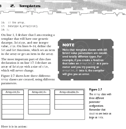
Copyeditor: Stephanie Koutek

Interior Layout: LJ Graphics, Susan Honeywell

Cover Design: Mike Tanamachi

Indexer: Kelly Talbot

Proofreader: Jenny Davidson

Microsoft, Windows, and Visual C++ are trademarks of Microsoft Corporation.Wolfenstein, Doom, and Quake are trademarks of Id Software, Inc. Warcraft and Starcraft are trademarks of Blizzard

Entertainment.

The artwork used in this book is copyrighted by its respective owners, and you may not use it in your own commercial works.

All other trademarks are the property of their respective owners.

Important: Premier Press cannot provide software support. Please contact the appropriate software manufacturer’s technical support line or Web site for assistance.

Premier Press and the author have attempted throughout this book to distinguish proprietary trade-marks from descriptive terms by following the capitalization style used by the manufacturer. Information contained in this book has been obtained by Premier Press from sources believed to be reliable. However, because of the possibility of human or mechanical error by our sources, Premier Press, or others, the Publisher does not guarantee the accuracy, adequacy, or completeness of any information and is not responsible for any errors or omissions or the results obtained from use of such information. Readers should be particularly aware of the fact that the Internet is an ever-chang-ing entity. Some facts may have changed since this book went to press.

ISBN: 1-931841-94-2

Library of Congress Catalog Card Number: 2002111226 Printed in the United States of America

03 04 05 06 07 BH 10 9 8 7 6 5 4 3 2 1

Premier Press, a division of Course Technology 2645 Erie Avenue, Suite 41

(7)

(8)

Acknowledgments

I

would first like to thank my family for putting up with me for the past nine months. Yes, yes, I’ll start cleaning the house now.

I would like to thank all of my friends at school: Jim, James, Dan, Scott, Kevin, and Kelvin, for helping me get through all of those boring classes without falling asleep. I would like to thank everyone at work for supporting me through this endeavor. I especially want to thank Ernest Pazera, André LaMothe, and everyone else at Premier Press for giving me this tremendous opportunity and believing in me. I would like to thank Bruno Sousa for opening the door to writing for me. I want to thank the pioneers of Gamedev.net, Kevin Hawkins and Dave Astle, for paving the road for me and making a book such as this possible.

I would like to thank all of you in the #gamedev crew, specifically (in no particular order) Trent Polack, Evan Pipho, April Gould, Joseph Fernald, Andrew Vehlies, Andrew Nguyen, John Hattan, Ken Kinnison, Seth Robinson, Denis Lukianov, Sean Kent, Nicholas Cooper, Ian Overgard, Greg Rosenblatt, Yannick Loitière, Henrik Stuart, Chris Hargrove, Richard Benson, Mat Noguchi, and everyone else! I would like to thank my artists, Steven Seator and Ari Feldman, who made this book’s demos look so much better than they would have been.

(9)

About the Author

Ron Penton’s lifelong dream has always been to be a game programmer. From the age of 11, when his parents bought him his first game programming book on how to make adventure games, he has always striven to learn the most about how games work and how to create them.

(10)

Contents at a Glance

Introduction

. . . xxxii

Part One

Concepts. . . 1

Chapter 1 Basic Algorithm Analysis

. . . 3

Chapter 2 Templates . . . 13

Part Two

The Basics. . . 37

Chapter 3 Arrays . . . 39

Chapter 4 Bitvectors. . . 83

Chapter 5 Multi-Dimensional Arrays . . . 107

Chapter 6 Linked Lists . . . 147

Chapter 7 Stacks and Queues . . . 189

Chapter 8 Hash Tables . . . 217

Chapter 9 Tying It Together: The Basics. . . 241

Part Three

Recursion and Trees . . . 315

Chapter 10 Recursion

. . . 317

Chapter 11 Trees . . . 329

Chapter 12 Binary Trees . . . 359

Chapter 13 Binary Search Trees. . . 389

(11)

ix

Contents at a Glance

Chapter 15 Game Trees and Minimax Trees

. . . 431

Chapter 16 Tying It Together: Trees . . . 463

Part Four

Graphs . . . 477

Chapter 17 Graphs . . . 479

Chapter 18 Using Graphs for AI: Finite State

Machines. . . 529

Chapter 19 Tying It Together: Graphs . . . 563

Part Five

Algorithms . . . 597

Chapter 20 Sorting Data . . . 599

Chapter 21 Data Compression

. . . 645

Chapter 22 Random Numbers . . . 697

Chapter 23 Pathfinding . . . 715

Chapter 24 Tying It Together: Algorithms . . . 769

Conclusion

. . . 793

Part Six

Appendixes . . . 799

Appendix A

A C++ Primer . . . 801

Appendix B

The Memory Layout of a Computer

Program . . . 835

Appendix C

Introduction to SDL. . . 847

Appendix D

Introduction to the Standard Template

Library . . . 879

(12)

Letter from the Series Editor . . . xxx

Introduction . . . xxxii

Part One

Concepts. . . 1

Chapter 1 Basic Algorithm Analysis . . . 3

A Quick Lesson on Algorithm Analysis . . . 4

Big-O Notation . . . 4

Comparing the Various Complexities. . . 9

Graphical Demonstration: Algorithm Complexity . . . 10

Conclusion . . . 11

Chapter 2 Templates . . . 13

What Are Templates?. . . 14

Template Functions . . . 15

Doing It the Old Way . . . 15

Doing It with Templates . . . 17

Template Classes . . . 19

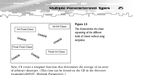
Multiple Parameterized Types . . . 24

Using Values as Template Parameters . . . 27

Using Values of a Specific Datatype . . . 27

(13)

xi

Part Two

The Basics. . . 37

Chapter 3 Arrays . . . 39

What Is an Array? . . . 40

Graphical Demonstration: Arrays . . . 41

Increasing or Decreasing Array Size . . . 43

Inserting or Removing an Item . . . 43

Native C Arrays and Pointers . . . 43

Static Arrays . . . 43

Dynamic Arrays . . . 49

An Array Class and Useful Algorithms . . . 59

The Data . . . 59

The Constructor . . . 59

The Destructor . . . 60

The Resize Algorithm . . . 60

The Access Operator . . . 62

The Conversion Operator. . . 63

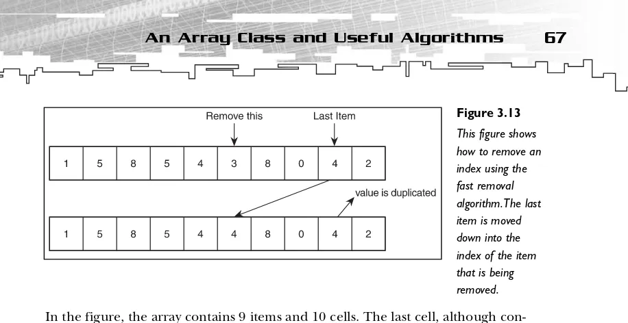
Inserting an Item Between Two Existing Items . . . 64

Removing an Item from the Array . . . 65

A Faster Removal Method . . . 66

Retrieving the Size of an Array . . . 67

Example 3-3. . . 67

Storing/Loading Arrays on Disk . . . 68

Writing an Array to Disk . . . 69

Reading an Array from Disk. . . 70

(14)

Application: Using Arrays to Store Game Data . . . 71

The Monster Class . . . 72

Declaring a Monster Array. . . 72

Adding a Monster to the Game. . . 72

Making a Better Insertion Algorithm . . . 73

Removing a Monster from the Game . . . 74

Checking for Monster Removal . . . 75

Playing the Game . . . 76

Analysis of Arrays in Games . . . 77

Cache Issues . . . 77

Resizing Arrays . . . 80

Inserting/Removing Cells . . . 80

Chapter 4 Bitvectors . . . 83

What Is a Bitvector? . . . 84

Graphical Demonstration: Bitvectors . . . 85

The Main Screen . . . 86

Using the Buttons . . . 86

Creating a Bitvector Class. . . 86

The Data . . . 87

The Resize Algorithm . . . 88

The Access Operator . . . 89

The Set Function . . . 91

The ClearAll Function . . . 93

The SetAll Function . . . 93

The WriteFile Function . . . 94

The ReadFile Function . . . 94

(15)

xiii

Chapter 5 Multi-Dimensional Arrays

. . . 107

What Is a Multi-Dimensional Array? . . . 108

Graphical Demonstration . . . 111

Native Multi-Dimensional Arrays. . . 112

Declaring a Multi-Dimensional Array . . . 112

Accessing a Multi-Dimensional Array . . . 115

Inside a Multi-Dimensional Array . . . 116

Dynamic Multi-Dimensional Arrays . . . 121

The Array2D Class . . . 121

The Array3D Class . . . 127

Application: Using 2D Arrays as Tilemaps . . . 131

Storing the Tilemap . . . 133

Generating the Tilemap . . . 134

Drawing the Tilemap . . . 135

Application: Layered Tilemaps. . . 136

Redefining the Tilemap. . . 138

Reinitializing the Tilemap . . . 139

(16)

Comparing Performance . . . 142

Comparing Size . . . 144

Analysis of Multi-Dimensional Arrays in Games. . . 144

Chapter 6 Linked Lists . . . 147

What Is a Linked List? . . . 148

Singly Linked Lists . . . 149

Graphical Demonstration: Singly Linked Lists. . . 149

Structure . . . 150

Example 6-4. . . 168

Final Thoughts on Singly Linked Lists . . . 169

Doubly Linked Lists . . . 169

Graphical Demonstration: Doubly Linked Lists . . . 170

Creating a Doubly Linked List . . . 171

Doubly Linked List Algorithms . . . 172

Reading and Writing Lists to Disk . . . 174

Writing a Linked List . . . 174

Reading a Linked List . . . 175

Application: Game Inventories . . . 176

The Player Class . . . 177

The Item Class . . . 177

Adding an Item to the Inventory . . . 178

Removing an Item from the Inventory . . . 178

Playing the Demo . . . 179

Application: Layered Tilemaps Revisited . . . 180

Declaring the Tilemap . . . 181

Creating the Tilemap . . . 182

Drawing the Tilemap . . . 182

Analysis and Comparison of Linked Lists . . . 184

(17)

xv

Chapter 7 Stacks and Queues . . . 189

Stacks . . . 190

What Is a Stack? . . . 190

Graphical Demonstration: Stacks . . . 192

The Stack Functions . . . 193

Implementing a Stack . . . 193

Application: Game Menus . . . 199

Queues . . . 204

Graphical Demonstration: Queues. . . 204

The Queue Functions . . . 206

Implementing a Queue . . . 206

Application: Command Queues . . . 212

Chapter 8 Hash Tables

. . . 217

What Is Sparse Data? . . . 218

The Basic Hash Table . . . 219

Collisions. . . 221

Hashing Functions . . . 221

Enhancing the Hash Table Structure . . . 224

Linear Overflow . . . 224

Quadratic Overflow . . . 225

Linked Overflow . . . 225

Graphical Demonstration: Hash Tables . . . 226

(18)

The HashEntry Class . . . 228

The HashTable Class . . . 229

Example 8-1: Using the Hash Table. . . 233

Application: Using Hash Tables to Store Resources . . . 235

The String Class . . . 236

Using the Table . . . 237

How the Demo Loads Resources . . . 237

Chapter 9 Tying It Together: The Basics . . . 241

Why Classes Are Good . . . 242

Storing Data in a Class . . . 243

Hiding Data . . . 245

Inheritance. . . 248

Using the Classes in a Game . . . 260

Making a Game . . . 265

Adventure:Version One . . . 266

Game 2—The Map Editor . . . 310

Part Three

Recursion and Trees . . . 315

Chapter 10 Recursion . . . 317

What Is Recursion? . . . 318

A Simple Example: Powers . . . 319

The Towers of Hanoi . . . 320

The Rules . . . 321

(19)

xvii

Chapter 11 Trees

. . . 329

What Is a Tree? . . . 330

The Recursive Nature of Trees . . . 332

Common Structure of Trees . . . 332

Graphical Demonstration:Trees . . . 333

Tutorial . . . 336

Building the Tree Class. . . 338

The Structure . . . 339

The Destroy Function . . . 341

The Count Function . . . 342

The Tree Iterator . . . 342

The Basic Iterator Functions . . . 343

The Vertical Iterator Functions . . . 345

The Horizontal Iterator Functions . . . .346

The Other Functions . . . 346

Building a Tree . . . 347

Top Down . . . 347

Bottom Up . . . 347

Traversing a Tree . . . 347

The Preorder Traversal . . . 348

The Postorder Traversal. . . 350

(20)

Game Demo 11-1: Plotlines . . . 352

Using Trees to Store Plotlines . . . 354

Chapter 12 Binary Trees

. . . 359

What Is a Binary Tree?. . . 360

Fullness . . . 361

Denseness . . . 361

Balance . . . 362

Structure of Binary Trees. . . 362

Linked Binary Trees . . . 362

Arrayed Binary Trees . . . 363

Graphical Demonstration: Binary Trees . . . 366

Coding a Binary Tree . . . 368

The Destructor and the Destroy Function . . . 369

The Count Function . . . 370

Using the BinaryTree Class . . . 370

Traversing the Binary Tree. . . 371

The Preorder Traversal . . . 372

The Postorder Traversal. . . 372

The Inorder Traversal. . . 372

Graphical Demonstration: Binary Tree Traversals . . . 373

Application: Parsing . . . 374

Arithmetic Expressions . . . 376

Parsing an Arithmetic Expression . . . 376

Recursive Descent Parsing. . . 377

(21)

xix

Chapter 13 Binary Search Trees . . . 389

What Is a BST? . . . 390

Inserting Data into a BST . . . 391

Finding Data in a BST . . . 394

Removing Data from a BST . . . 394

The BST Rules . . . 394

Sub-Optimal Trees . . . 395

Graphical Demonstration: BSTs . . . 395

Coding a BST . . . 397

Comparison Functions. . . 397

The Insert Function . . . 399

The Find Function . . . 400

Example 13-1: Using the BST Class . . . 401

Application: Storing Resources, Revisited . . . 402

The Resource Class. . . 402

The Comparison Function . . . 403

Inserting Resources . . . 403

Finding Resources . . . 403

Chapter 14 Priority Queues and Heaps . . . 407

What Is a Priority Queue? . . . 408

What Is a Heap?. . . 410

Why Can a Heap Be a Priority Queue? . . . 411

Graphical Demonstration: Heaps . . . 417

(22)

The Structure . . . 419 The Constructor . . . 419 The Enqueue Function . . . 420 The WalkUp Function . . . 420 The Dequeue Function . . . 422 The WalkDown Function . . . 422

Application: Building Queues. . . 424

The Units . . . 426 Creating a Factory . . . 426 The Heap . . . 427 Enqueuing a Unit . . . 427 Starting Construction . . . 428 Completing Construction . . . 428 Playing the Demo . . . 429

Chapter 15 Game Trees and Minimax Trees . . . 431

What Is a Game Tree? . . . 432 What Is a Minimax Tree? . . . 434 Graphical Demonstration: Minimax Trees . . . 437 Game States. . . 439 More Complex Games. . . 442 Application: Rock Piles. . . 442

The Game State . . . 443 The Global Variables . . . 445 Generating the Game Tree . . . 446 Simulating Play . . . 452 Playing the Game . . . 454

More Complex Games. . . 456

(23)

xxi

Chapter 16 Tying It Together: Trees . . . 463

Expanding the Game . . . 464

Altering the Map Format . . . 465 Game Demo 16-1: Altering the Game . . . 466 The Map Editor . . . 473

Further Enhancements . . . 475 Conclusion . . . 475

Part Four

Graphs . . . 477

Chapter 17 Graphs . . . 479

What Is a Graph? . . . 480

Linked Lists and Trees . . . 480 Graphs. . . 482 Parts of a Graph . . . 482

Types of Graphs . . . 482

Bi-Directional Graphs . . . 483 Uni-Directional Graphs . . . 483 Weighted Graphs. . . 484 Tilemaps . . . 485

Implementing a Graph. . . 486

Adjacency Tables . . . 486 Direction Tables . . . 488 General-Purpose Linked Graphs . . . 489

(24)

The Depth-First Search . . . 493 The Breadth-First Search . . . 495 A Final Word on Graph Traversals . . . 499 Graphical Demonstration: Graph Traversals . . . 500

The Graph Class . . . 501

The GraphArc Class . . . 501 The GraphNode Classes . . . 502 The Graph Class . . . 504

Application: Making a Direction-Table Dungeon . . . 512

The Map . . . 512 Creating the Map. . . 513 Drawing the Map . . . 514 Moving Around the Map . . . 516 Playing the Demo . . . 517

Application: Portal Engines . . . 518

Sectors . . . 519 Determining Sector Visibility . . . 521 Coding the Demo . . . 522 Playing the Demo . . . 527

Chapter 18 Using Graphs for AI: Finite State

Machines . . . 529

What Is a Finite State Machine? . . . 530 Complex Finite State Machines. . . 533 Implementing a Finite State Machine . . . 535 Graphical Demonstration: Finite State Machines . . . 537 Even More Complex Finite State Machines . . . 538

(25)

xxiii

Chapter 19 Tying It Together: Graphs . . . 563

The New Map Format . . . 564

The New Room Entry Structure . . . 565 The File Format . . . 566

Game Demonstration 19-1: Adding the New Map Format . . . 567

The DirectionMap . . . 568 Changes to the Game Logic . . . 580 Playing the Game . . . 582

Converting Old Maps . . . 583 The Directionmap Map Editor. . . 584

The Initial Map. . . 585 Setting and Clearing Tiles. . . 586 Loading a Map . . . 588 Saving a Map . . . 590 Using the Editor . . . 593

Upgrading the Tilemap Editor . . . 594

The Save Function . . . 594 The Load Function . . . 595

(26)

Part Five

Algorithms . . . 597

Chapter 20 Sorting Data . . . 599

The Simplest Sort: Bubble Sort. . . 600

Worst-Case Bubble Sort . . . 601 Graphical Demonstration: Bubble Sort . . . 602 Coding the Bubble Sort . . . 604

The Hacked Sort: Heap Sort . . . 609

Graphical Demonstration: Heap Sort. . . 611 Coding the Heap Sort . . . 613

The Fastest Sort: Quicksort . . . 616

Picking the Pivot . . . 616 Performing the Quicksort . . . 618 Graphical Demonstration: Quicksort . . . 621 Coding the Quicksort . . . 623

Graphical Demonstration: Race. . . 627 The Clever Sort: Radix Sort . . . 630

Graphical Demonstration: Radix Sorts. . . 631 Coding the Radix Sort . . . 633

Other Sorts . . . 637 Application: Depth-Based Games . . . 638

The Player Class . . . 639 The Globals . . . 640 The Player Comparison Function. . . 640 Initializing the Players. . . 640 Sorting the Players. . . 641 Drawing the Players. . . 641 Playing the Game . . . 642

(27)

xxv

Chapter 21 Data Compression. . . 645

Why Compress Data? . . . 646

Data Busses . . . 647 The Internet . . . 649

Run Length Encoding . . . 649

What Kinds of Data Can Be Used for RLE?. . . 650 Graphical Demonstration: RLEs . . . 651 Coding an RLE Compressor and Decompressor . . . 656

Huffman Trees . . . 665

Huffman Decoding. . . 665 Creating a Huffman Tree . . . 667 Coding a Huffman Tree Class. . . 676 Example 21-3. . . 691 Test Files . . . 692 Example 21-4. . . 693

Data Encryption . . . 693 Further Topics in Compression . . . 694 Conclusion . . . 694

Chapter 22 Random Numbers . . . 697

Generating Random Integers . . . 698

Generating Random Numbers in a Program . . . 699 Using rand and srand. . . 700 Using a Non-Constant Seed Value . . . 702 Generating a Random Number Within a Range . . . 702

Generating Random Percents . . . 705 Generating Random Floats . . . 706 Generating Non-Linear Random Numbers. . . 707

(28)

Adding Three Random Numbers . . . 711 Graphical Demonstration: Random Distribution Graphs . . . 712

Chapter 23 Pathfinding. . . 715

Basic Pathfinding . . . 716

Random Bouncing . . . 718 Object Tracing . . . 719

Robust Pathfinding . . . 721

The Breadth-First Search . . . 721 Making a Smarter Pathfinder . . . 739 Making a Better Heuristic . . . 746 The A* Pathfinder . . . 750 Graphical Demonstration: Path Comparisons . . . 753

Weighted Maps . . . 754

Application: Stealth . . . 756

Thinking Beyond Tile-Based Pathfinding . . . 762

Line-Based Pathfinding . . . 762 Quadtrees . . . 764 Waypoints . . . 765

Chapter 24 Tying It Together: Algorithms

. . . 769

Making the Enemies Smarter with Pathfinding . . . 770

(29)

xxvii

Conclusion

. . . 793

Extra Topics . . . 794 Further Reading and References . . . 795

Data Structure Books . . . 795 C++ Books . . . 796 Game Programming Books . . . 797 Web Sites . . . 798

Part Six

Appendixes . . . 799

Appendix A

A C++ Primer . . . 801

Basic Bit Math . . . 802

Binary Numbers . . . 802 Computer Storage. . . 805 Bitwise Math . . . 807 Bitwise Math in C++ . . . 807 Bitshifting. . . 809

Standard C/C++ Functions Used in This Book . . . 811

Basic Input/Output . . . 811 File I/O . . . 814 Math Functions . . . 817 The Time Function. . . 818 The Random Functions . . . 819

Exceptions and Error Handling . . . 820

Assertions . . . 820 Return Codes . . . 820 Exceptions . . . 821

(30)

Class Topics. . . 824

Constructors . . . 824 Destructors . . . 826 Operator Overloads . . . 827 Conversion Operators . . . 829 The This Pointer . . . 830 Inline Functions . . . 830 Function Pointers . . . 832

Appendix B

The Memory Layout of a

Computer Program . . . 835

The Memory Sections . . . 836 The Code Memory. . . 837 The Global Memory. . . 838

Global Variables . . . 838 Static Variables . . . 839

The Stack . . . 840

Local Variables . . . 840 Parameters . . . 842 Return Values. . . 843

The Free Store. . . 844 Conclusion . . . 845

Appendix C

Introduction to SDL . . . 847

The Licensing . . . 848 Setting Up SDL . . . 849

(31)

xxix

Appendix D

Introduction to the Standard

Template Library . . . 879

STLPort . . . 880 STL Versus This Book. . . 882 Namespaces . . . 883 The Organization of STL . . . 885 Containers . . . 889

Sequence Containers . . . 890 Associative Containers . . . 896 Container Adaptors . . . 896 The Miscellaneous Containers . . . 898

(32)

Letter from the

Series Editor

Dear reader,

I’ve always wanted to write a book on data structures. However, there is simply no way to do the job right unless you use graphics and animation, and that means a lot of work. I personally think that all computer books will be animated, annotated, and interactive within 10 years—they have to be. There is simply too much information these days to convey with text alone; we need to use graphics, color, sound, animation—anything and everything to try to make the complex computer science subjects under-standable these days.

With that in mind, I wanted a data structures book that was like no

other—a book using today’s technology that could live up to my high stan-dards. So I set out to find the perfect author and finally Ron Penton came along to take on the challenge. Ron, too, had my same vision for a data structures book. We couldn’t do something that had been done—there are a zillion boring data structure books—but if we could apply gaming tech-nology and graphics to teach the subject, we would have something unique. Moreover, this book is for anyone who wants to learn data struc-tures and related important algorithms. Sure, if you’re a game program-mer then you will feel at home, but if you’re not, then believe me, put down that hardbound college text and pick this book up because not only will you absolutely know this stuff inside and out by the time you’re done, but you will have an image in your mind like you have never had before. All right, now I want to talk about what you’re going to find inside.

(33)

xxxi

Letter from the Series Editor

pull this off. On the other hand, if you are a game programmer, then you will greatly appreciate Ron’s insight into applications of various data struc-tures and algorithms for game-related programs. In fact, he came up with some pretty cool applications I hadn’t thought of!

So what’s inside? Well, the book starts off with an introduction, gets you warmed up with arrays, bit vectors, and simple stuff like that, and talks about the use of SDL (the simple direct media layer) used for the demos. Then the book drives a steak through the heart of the data structure drag-on and covers asymptotic analysis, linked lists, queues, heaps, binary trees, graphs, hash tables, and the list goes on and on. After Ron has made you a believer that hash tables are the key to the universe, he switches gears to algorithms and covers many of the classic algorithms in computer science, such as sorting, searching, compression, and more. Of course, no book like this would be complete without coverage of recursion, and that’s in here, too—but you will love it because for once, you will be able to see the recursion! Finally, the book ends with primers on C++, SDL, and the stan-dard template library, so basically you will be a data structure god when you’re done!

In conclusion, this book is for the person who is looking for both a practi-cal and a theoretipracti-cal base in data structures and algorithms. I guarantee that it will get you farther from ground zero than anything else.

(34)

Introduction

What is a computer program? When you get down to the lowest level, you can sepa-rate a program into two main sections: the data and the instructions that opesepa-rate on the data. These two sections of a program are commonly called the data struc-tures and the algorithms.

This book will teach you how to create many data structures, ranging from the very simple to the moderately complex.

Understanding data structures and algorithms is an essential part of game pro-gramming. Knowing the most efficient way to store data and work with the data is an important part of game programming; you want your games to run as quickly as possible so you can pack as many cool features into them as you can.

I have a few goals with this book:

■ _{Teach you how the most popular data structures and algorithms work} ■ _{Teach you how to make the structures and algorithms}

■ _{Teach you how to use the data structures in computer games}

Mark Twain once said this:

It is a good thing, perhaps, to write for the amusement of the public. But it is a far higher and nobler thing to write for their instruction.

(35)

xxxiii

Introduction

Who Is This Book For?

If you’re standing in the bookstore reading this Introduction and wondering, “Is this book good for me?”, then read this section. If you’ve already bought the book, thank you! I am going to assume that you’re reading this book because you want to learn more (unless some diabolical person is forcing you to read this as an arcane form of torture...).

This is a somewhat complex book because it deals with lots of concepts. However, I feel that I have included ample introductory material as well. Therefore, this book is for the game programmer who is just starting out at an intermediate level. So what do I expect you to know?

I expect you to know basic C++, but don’t feel confused if you don’t feel like an expert. Pretty much every complex topic I use in C++ is covered in Appendix A, so if you’re unfamiliar with a concept or just forget how something works, take a few minutes to read that appendix.

The most complex feature of C++ that I use is templates, but you don’t need to know about them before you read this book. Chapter 2 is an extensive introduction to templates, so don’t worry if you don’t know what they are just yet.

One advanced concept I use often in the later parts of the book is recursion, but you don’t have to know about that, either. Chapter 10 is a small introduction to recursion.

This book is for anyone who wants to learn more about how a computer works, how to store data, and how to efficiently work on that data. All of this material is essential to game programming, so take a glance at the Table of Contents. If there is anything there that you don’t already know about, this book is for you. Even if you know a little about the topics, this book is still good for you because every chapter goes in depth about these subjects.

Topics Covered in This Book

In this book, I cover many data structures and how to use them in games, ranging from the simple (arrays) to the complex (graphs and trees).

(36)

understand how it works. These demonstrations all use the Simple DirectMedia Layer (SDL) multimedia library, which I go more into depth on in just a little bit. All of these demonstrations are located in the \demonstrations\ directory on the CD. After that, I show you how to actually code the structure or algorithm in C++. The code for these sections is mostly platform free, so it will usually compile on any compiler. I mention any sections that are platform-specific in the book. All of the code for the data structures and algorithms can be found on the CD in the directory \structures\ for your convenience. Copies of the files have also been placed in the directories of every demo that uses them. Whenever necessary, I have included console mode Examples on how these structures work in the \examples\ directory on the CD. All of the examples use pure C/C++, with no extra SDKs or APIs needed, so they use input and output to the text console window on your computer.

CAUTION

You are free to use any of the data structures included on the CD in any projects you use. However, be warned; they were designed to demonstrate the structures and are not super-optimized. Many functions can be made faster, particularly the small functions that can be inlined (see Appendix A).You cannot copy any of the structures because none of them implements proper copy constructors.

Whenever you pass a structure into a function as a parameter, make absolutely certain that you pass-by-reference or use a pointer; otherwise, it will mess up your structure. If you don’t know what this means just yet, look at the functions that use the data structures; they demonstrate how to use them correctly.

Finally, I show you an interactive Game Demonstration, which highlights the usage of the structure or algorithm in a game-like atmosphere. Most of these games are sim-ple, but they prove a point. These demonstrations also use the SDL multimedia library and are located on the CD in the directory \demonstrations\ .

Some chapters might deviate from the format to show you different versions of the structures.

(37)

xxxv

Introduction

■ _Concepts ■ _{The Basics}

■ _{Recursion and Trees} ■ _Graphs

■ _Algorithms ■ _Appendixes

Concepts

In this part, I introduce you to some of the concepts used when dealing with data structures and algorithms. You might know some of them, or you might not.

■ _{Basic Algorithm Analysis—This chapter is a little on the theoretical side, and}

it deals with topics that are usually taught in school. This chapter shows you how algorithms are rated for speed so that you can see how to choose the best algorithm for your needs.

■ _{Templates—This is a somewhat advanced C++ concept. Some C++ books}

don’t cover templates well, and because this book uses them extensively, I feel that it is a good idea to include a chapter on how to use them. You can safely skip this section if you already know the material.

The Basics

In this part, I show you many of the basic data structures used within games and how to use them. These include

■ _{Arrays—This chapter teaches you everything you ever needed to know about}

arrays. You might not think arrays need this much explaining, but they are an important structure in computing.

■ _{Bitvectors—Bitvectors are an important part of space optimization. This}

chapter shows you how to store data in as small of a place as possible.

■ _{Multi-Dimensional Arrays—This chapter expands on the array chapter and}

shows you how to use arrays with more than one dimension.

■ _{Linked Lists—This chapter introduces you to the concept of linked data,}

(38)

■ _{Stacks and Queues—This is the first chapter that doesn’t introduce you to a}

new structure. Instead, it shows you how to access data in certain ways.

■ _{Hash Tables—This chapter shows you an advanced method of storing data by}

using both arrays and linked lists. It is the last structure covered in this part of the book.

In addition to those, the last chapter in this part (Chapter 9) is the first of the “Tying It Together” chapters. There are four of these chapters throughout the book, one at the end of Parts Two, Three, Four, and Five. In Chapter 9, I introduce you to the ideas of learning how to store custom game data and designing your own classes. After that, I show you how to design a basic game using many of the structures from this part of the book.

Recursion and Trees

In this Part, I introduce you to the ideas of recursion, recursive algorithms, and recursive data structures, namely trees. This Part includes the following chapters:

■ _{Recursion—This is a small chapter introducing you to the idea of recursion}

and how it works. Recursion is a tough subject and isn’t covered well in most C++ books, so I felt that I needed to include an introduction to the concept.

■ _{Trees—This chapter introduces you to the idea of a linked tree data}

struc-ture and how it is used.

■ _{Binary Trees—This chapter shows you a specific subset of trees. Binary trees}

are the most frequently used tree structures in computing.

■ _{Binary Search Trees—This chapter shows you how to store data in a recursive}

manner so that you can access it quickly later.

■ _{Priority Queues and Heaps—Heaps are another variation of the binary tree.}

This chapter shows you how to use a binary tree to implement an efficient queue variation called the priority queue.

■ _{Game Trees and Minimax Trees—Game Trees are a different kind of tree}

used to store state information about turn-based games.

(39)

xxxvii

Introduction

Graphs

In this part, I introduce you to the graph data structure, which is another linked data structure that is somewhat like trees. This part of the book is broken down into the following chapters:

■ _{Graphs—This chapter introduces you to the idea of the graph structure and}

its many derivatives. Graphs are used all over in game programming.

■ _{Using Graphs for AI: Finite State Machines—This is an application of the}

graph data structure to the field of artificial intelligence—a way to make your games smarter.

Chapter 19 applies some concepts from the graph chapter and adds them to the game from Chapter 16.

Algorithms

Originally, I had planned to include these topics in the previous three parts, but they really fit better in a section of their own. Some of the topics use concepts from all three of the previous parts, and others don’t. This part is composed of the fol-lowing chapters:

■ _{Sorting Data—This chapter covers four different sorting algorithms.} ■ _{Data Compression—This chapter shows you two ways to compress data.} ■ _{Random Numbers—This chapter shows you how to use the random number}

generator built into the C standard library and how to use some algorithms to get impressive results from generating random numbers.

■ _{Pathfinding—This chapter shows you four different pathfinding algorithms}

to use on the maps you create in your games.

The final chapter, Chapter 24, expands on the game from Chapters 9, 16, and 19 by adding pathfinding support to the AIs in the game.

Appendixes

Finally, there are four appendixes in the book that cover a variety of topics:

■ _{A C++ Primer—This appendix attempts to cover the features of C++ that are}

(40)

■ _{The Memory Layout of a Computer Program—To understand how to use a}

computer to its fullest extent, you must know about how it structures its memory. This appendix tells you this information.

■ _{Introduction to SDL—This is a basic introduction to the Simple DirectMedia}

Layer library, which the book uses for all of the demonstrations. It also goes over the two SDL libraries I’ve developed to make the demonstrations in the book.

■ _{Introduction to the Standard Template Library—This appendix introduces}

you to the C++ Standard Template Library, which is a built-in structure and algorithm library that should come with every compiler.

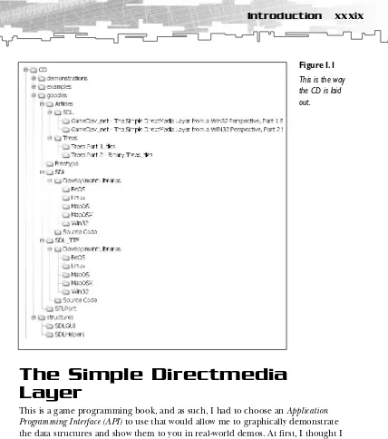
What’s on the CD?

The CD for this book contains every Example, Game Demonstration, and Graphical Demonstration for the book. There are 33 Examples, 26 Game Demonstrations, and 34 Graphical Demonstrations. That is 93 examples and demonstrations! That should be enough to keep you busy for a while.

Just in case you end up wanting more, however, there’s even more stuff on the CD. There are 19 code files full of the data structures and algorithms in this book, con-veniently located in the directory \structures\, as well as the two SDL libraries I’ve developed for the book (see Appendix C).

In the \goodies\ directory, there are four articles—two dealing with trees and two dealing with SDL. They expand on the topics covered in this book.

In addition, the SDL, SDL_TTF, STLPort, and FreeType libraries (see Appendixes C and D for more information) are in that directory.

(41)

xxxix

Introduction

[image:41.513.29.457.20.504.2]

the CD is laid out.

Figure I.1

This is the way

The Simple Directmedia

Layer

(42)

A friend of mine recently introduced me to a very simple API called SDL: The Simple Directmedia Layer. I think that the S part of the title should be emphasized because the API is simple. I was able to make a working SDL program (no, it wasn’t “Hello World”. It’s the Array Demonstration from Chapter 3) in less than an hour after first looking at the header files. It truly is that simple.

Therefore, I decided that SDL was the API I wanted to use to demonstrate the con-cepts in this book. It’s simple enough so that it will not get in the way of the theory, and I am confident that you will be able to pick it up in almost no time at all. I’ve provided a simple primer for SDL in Appendix C to get you started with it. So if you get confused by the graphics code, just take a peek at Appendix C. I promise, the book won’t go anywhere until you return.

Coding Conventions Used in

This Book

Although the point of this book is to demonstrate how to effectively organize your data, organizing your code is still somewhat important. Because of this, I will be adopting a simple coding standard.

In an effort to emphasize the scope of the different variables within the book, I have used a simple mutation of the popular Hungarian Notation:

■ _{Global variables will be prefixed with}g_.

Examples: g_name, g_state

■ _{Class/Structure member variables will be prefixed with}m_.

Examples: m_name, m_state

■ _{Parameter variables will be prefixed with}p_.

Examples: p_name, p_state

■ _{Local function variables have no prefix.}

Examples: name, state

Besides the prefix, all variables will be lowercase.

Class and function names will be title-cased, with each major word in the name

capitalized.

(43)

xli

Introduction

Artwork

Two people provided the artwork used for the demos in this book. First and fore-most, I would like to thank Steve Seator for making all of the person sprites and weapon icons in the game demos. He has an excellent Web site at http://www.spritedomain.net. If you’re interested in his artwork, I urge you to visit the site.

The other artist is Ari Feldman, who provided most of the other sprites in the demos. His Web site is http://www.arifeldman.com.

I would like to thank both of them, because without them, my game demos would be even cheesier than they already are.

All of the artwork is copyrighted by them, so you cannot use it in your own game projects.

Are You Ready?

(44)

(45)

PART ONE

(46)

1 Basic Algorithm Analysis

(47)

CHAPTER 1

Basic

Algorithm

(48)

A

lmost any computer science teacher would probably kill me for including this topic as such a small chapter. After all, entire books are dedicated to this subject. But we’re not computer science professors—we’re game programmers! We don’t care about all of this highly mathematical stuff, right? Well, that’s only half right. We should at least pay some attention to the algorithms we write. In this chapter, you will learn

■ _{How algorithms are rated for growth} ■ _{The most common complexity classes}

■ _{How each of the complexity classes compares to the others}

A Quick Lesson on

Algorithm Analysis

Some people spend their careers studying algorithms and data structures, and you should be thankful for them. These are the people who invented some of the nifty things you’ll be using in this book. These things are used because people have proven that they work. For those of us who don’t want to spend years proving that the efficiency of algorithm 1 is better than algorithm 2, this is a godsend.

However, I still think that at least some knowledge of how algorithms are analyzed is required. This section is meant to introduce you to the very basics of these con-cepts so that you can understand why some of the data structures and algorithms we use are better than others. Throughout the book, I refer to some of the termi-nology I’ve introduced here, so unless you already know a little about algorithm analysis, I beg you to please read this section.

Big-O Notation

Big-O notation is a helpful tool that computer scientists often use to help define the complexity of a function. Simply put, the Big-O of an algorithm is a function that roughly estimates how the algorithm scales when it is used on different sized datasets. Big-O notation is shown like this:

(49)

5 A Quick Lesson on Algorithm Analysis

The function is usually a mathematical formula based on the letters n and c, where

n represents the number of data elements in the algorithm and c represents a con-stant number.

Imagine having a huge collection of action figures—at least 1,000 of them. But you’re a very sloppy person, and you don’t have them organized in any manner at all. (Okay, maybe you’re not so sloppy, but just pretend.) Now, one of your friends comes over and wants to look at your exclusive Boba Fett action figure—the really rare one. In the worst-case scenario, you need to search through every single one of your figures because Boba Fett might be the 1000th figure in your collection. In this example, the Big-O of the search would be O(n), because the number of items to search is 1,000, and in the worst-case scenario, you have to search through every figure in the collection. (Technically, the worst case would be not finding him at all because your mom sold him for grocery money.) Of course, Boba Fett might be the first figure you look at or he might be the 500th, but when analyzing an algorithm, you don’t (usually) care about the best case because the best case only occurs in optimal conditions, which almost never occur.

A number of different functions are typically used to examine the complexity of an algorithm, and these are (listed in order from the lowest complexity to the highest complexity) constant, log2n, n, nlog2n, n2, n3, and 2

n

. It’s okay if you don’t know exactly what these functions do. Just look at the graphs that follow; they will show you visually how the function looks as the number of data items increases.

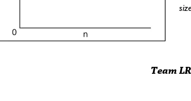
O(

c

)

[image:49.513.55.248.527.629.2]

As I stated before, the C in a Big-O expression is a constant. Figure 1.1 illustrates the constant function. The graphs produced by the constant function are all hori-zontal, meaning that no matter how large the dataset is, the algorithm will take the same amount of time to complete. These functions are usually considered the fastest. Some of the structures in this book have algorithms associated with them that approach O(c) as a best-case scenario.

Figure 1.1

(50)

O(Log

2

n

)

Figure 1.2 shows the logarithm base 2 function. In case you don’t know, a loga-rithm function is the inverse of an exponential function. The best way to describe it is this: In a base 2 logarithm, the vertical component is increased by 1 whenever the dataset size is doubled. The log of 1 is 0, the log of 2 is 1, the log of 4 is 3, the log of 8 is 4, and so on. Logarithm-based algorithms are generally considered the most efficient algorithms in existence that depend on the size of the data.

(Remember: O(c) algorithms don’t depend on the size of the data.)

Figure 1.2

The Log2n function varies with the size of

the data, but becomes more efficient as more data is added.

O(

n

)

O(n) is called the linear function. Figure 1.3 illustrates what this function looks like. Basically, an O(n) algorithm grows at a constant rate with the data size. This growth rate means that if an O(n) algorithm takes 20 seconds to operate on 1,000 data items, it would take roughly 40 seconds to operate on 2,000 data items. The scenario of trying to find the Boba Fett action figure is an example of an O(n) algorithm.

Figure 1.3

The linear function varies directly with the size of the data.Twice as much data will take twice as long to compute.

O(

n

log

2

n

)

(51)

7 A Quick Lesson on Algorithm Analysis

previous graphs, but compared to some of the more complex functions I discuss next, it is also considered a fairly efficient algorithm class.

Figure 1.4

The n log2n function varies with

the size of the data, but has a relatively shallow curve, which makes functions that fall into this category seem efficient.

O(

n

2

₎

This is where the more complex functions begin. An n2 _{function (shown in Figure}

1.5) is typically considered inefficient for most tasks because the function grows at an enormously high rate. For example, if it took 20 seconds to perform an algo-rithm on 1,000 data items, it would take 80 seconds for 2,000 items—4 times as long! In general, you should stay away from O(n2_{) algorithms unless you have no}

other choice. An example of an O(n2_{) function would be a for-loop with another}

for-loop nested inside.

Figure 1.5

The n2 _{function has a steep incline,}

(52)

O(

n

3

)

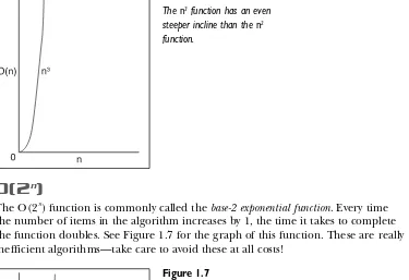
If you thought O(n2_{) was bad, O(}_n3_{) is even worse! Even though the graph looks}

almost identical to O(n2_{) (see Figures 1.5 and 1.6), it shoots up at a much higher}

[image:52.513.56.431.183.440.2]

rate. If it took 20 seconds to perform an algorithm on 1,000 items, it would take 160 seconds for 2,000 items! That’s 8 times longer!

Figure 1.6

The n3 _{function has an even}

steeper incline than the n2

function.

O(2

n

)

The O(2n

) function is commonly called the base-2 exponential function. Every time the number of items in the algorithm increases by 1, the time it takes to complete the function doubles. See Figure 1.7 for the graph of this function. These are really inefficient algorithms—take care to avoid these at all costs!

Figure 1.7

[image:52.513.55.206.459.635.2]

(53)

9 A Quick Lesson on Algorithm Analysis

O(2n

n3

n

) is faster than O(n3_).

NOTE

) algorithms are actually faster than O( ) algorithms for very small

datasets.This has to do with the way an O(2 ) algorithm slopes: It starts out slow, but shoots up quicker than all the other algorithms. For values of that are less than 10, O(2

Comparing the Various

Complexities

The following table is a comparison of the various functions that gives you a better understanding of how the complexity functions affect the running time of an algo-rithm. (This is a generic algorithm prediction that assumes it takes exactly 1 second to process each item.)

T

ABLE

16 Items 32 Items 64 Items 128 Items

O(log2n) 4 seconds 5 seconds 6 seconds 7 seconds

O(n) 16 seconds 32 seconds 64 seconds 128 seconds

O(nlog2n) 64 seconds 160 seconds 384 seconds 896 seconds

O(n2₎ _{256 seconds}

O(n3₎ _{73 hours}

O(2n

) 18 hours 500,000 millennia —————-*

1.1 Running Time Comparisons

Complexity

17 minutes 68 minutes 273 minutes

68 minutes 546 minutes 24 days

136 years

* My calculator doesn’t go this high.

As you can see, this table puts things in a better perspective. Even if you were to speed up a 2n

algorithm so that it spends a millisecond per item, it would still take millions of years to complete for 128 items. Isn’t that insane? I hope you under-stand now why algorithms should be analyzed carefully for their complexity. You could accidentally create an algorithm that takes too much time to complete—and not even realize it!

(54)

single loop on the same number of items. What would the complexity of this algo-rithm be? It is natural to assume that it would be O(n2₊_n_{), but that is incorrect.}

Remember, when you measure the complexity of an algorithm, you really care only about how it grows as the data size increases. Eventually, the single n term will be overpowered by the much larger n2 _{term and become insignificant. So the correct}

complexity of the algorithm is actually O(n2_).

Also, keep in mind that dividing or multiplying by a constant has no effect on the complexity of an algorithm. If you had an algorithm consisting of a single for-loop and it only processed half of the items, the algorithm would not be O(n/2). It would still be O(n) because the growth of the algorithm is still linear; doubling the number of items that the algorithm works on still doubles the amount of time taken to complete the algorithm.

I’m sorry to lay down so much mathematical buzz-speak so early in the book, but I feel that it’s important. If you walk away from this chapter having learned one thing, it should be the knowledge of which algorithm classes are generally faster than others.

Graphical Demonstration:

Algorithm Complexity

I’ve included a demonstration of the different complexity graphs on the CD-ROM that comes with this book. It’s a really simple program, and I encourage you to play around with it to gain an understanding of how the graphs of the functions look. The program is quite simple to understand, and you can find it in the \demonstra-tions\ch01\Demo01 - Algorithm Complexity\ directory on the CD.

Compiling the Demo

This demonstration uses the SDLGUI library that I have developed for the book. For more information about this library, see Appendix B, “The Memory Layout of a Computer Program.”

(55)

11 Conclusion

When you start the program, as shown in Figure 1.8, you see a graph, six check boxes, and four arrows.

Figure 1.8

This is a screenshot of the demonstration in action.

You can click on any of the check boxes to make a graph appear. You can click any combination at the same time, which enables you to compare the different graphs. The arrows adjust the graph axes. The up and down arrows increase and decrease the Y axis within a range of 10–5,000. The left and right arrows decrease and increase the X axis, also within a range of 10–5,000.

Conclusion

(56)

(57)

CHAPTER 2

(58)

I

n this chapter, you learn about templates. Templates are a fairly important con-cept in computer programming when you are dealing with data structures because they allow you to easily maintain your code. If you already know about templates, you can safely skip this chapter, but if you are not very good at them (or have never even heard of them), I’d advise you to read on. In this chapter, you will learn

■ _{What a template is}

■ _{How to create template functions} ■ _{How to create template classes}

■ _{How to use multiple template parameters} ■ _{How to use values as a template parameter} ■ _{The limitations and problems of templates} ■ _{How templates work under the hood}

What Are Templates?

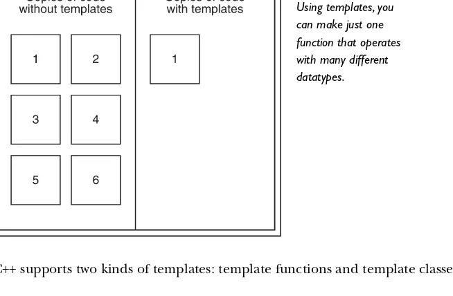
Templates are a relatively new concept in computer languages. A template is a soft-ware engineering tool that enables a programmer to reuse code on many different datatypes.

The best way to describe a template is as a pattern, or a mold, which will be reused over and over again. A real-world example would be the procedures of a company that manufactures figurines. First, the company produces a mold of the figure they want to produce. After that, they choose which material they want the figures made of, and then they use the mold to create the figure. With the same mold, they can make a figure out of plastic, pewter, iron, or even gold and silver.

(59)

15 Template Functions

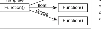
[image:59.513.55.382.186.400.2]

Say you want a specific algorithm to work on six different types of datatypes. Without templates, you would have to copy and paste the algorithm six times and manually change the datatypes in each copy! With templates, it is possible to make only one copy of the code and use that one copy over and over again. The algo-rithm on the right-hand side of Figure 2.1 is your mold, which allows you to make figurines of any type you want.

Figure 2.1

Using templates, you can make just one function that operates with many different datatypes.

C++ supports two kinds of templates: template functions and template classes.

Template Functions

A template function is a function that can operate on a generic datatype, which will allow you to use the same function on many different types of data.

Doing It the Old Way

(60)

NOTE

Although Chapter 3, “Arrays,” discusses arrays, I am introducing them a little bit earlier here. If you’re reading this book, you should probably know a little bit about arrays already. However, if you don’t know about them, you may want to skip ahead and read the first part of Chapter 3 and then come back here.

1: int SumIntegers( int* p_array, int p_count ) 2: {

3: int index; 4: int sum = 0;

5: for( index = 0; index < p_count; index++ ) 6: sum += p_array[index];

7: return sum; 8: }

Line 3 defines the index variable, which will be used to access each item in p_array. On line 4, I define the sum variable, which is initially empty, and on lines 5 and 6, we loop through the array, adding each index to the sum. Lastly, on line 7, the sum is returned.

A little further down the line, you might want to do the same thing, but with floats. Without templates, you would probably just copy the code and replace the ints with floats, like this:

1: float SumFloats( float* p_array, int p_count ) 2: {

3: int index; 4: float sum = 0;

7: return sum; 8: }

(61)

17 Template Functions

Doing It with Templates

C++ comes to the rescue by allowing us to create template functions, which use the same algorithm but operate on different datatypes. The syntax for a template func-tion is such:

template< class T >

returntype functionname( parameter list )

You first declare that you are creating a template by putting in the template key-word. You then put the class keyword and the name of the generic datatype after that, contained within the <> brackets. In the preceding example, T (which stands for “Template”) is the name of the generic datatype, and whenever I want to use the class in the function, I refer to it as T. After that, you write the function declara-tion the same way you normally would. In my examples, I separate the template declaration and the function

declara-tion into two lines, but you aren’t required to do that. Technically, they can be on the same line, but I prefer separating them because it makes the code more readable.

Let’s look at an example of a template

function by condensing the two sum functions into one template function called

sum:

T is called a in the

NOTE

parameterized type

world of software engineering.

1: template< class T >

2: T Sum( T* p_array, int p_count ) 3: {

4: int index; 5: T sum = 0;

8: return sum; 9: }

On line 1, I use the template keyword to tell the compiler that I am creating a tem-plate function that will have one generic datatype as a parameter, henceforth

(62)

a template function that calls its

foo foo

CAUTION

It is essential, upon choosing a name for your generic datatype within the template, that you choose one that does not conflict with an existing class name. For example, if you have generic class , but you also have a regular class named , the compil-er won’t like this and will barf compil-error messages all over you.

On line 2, I declare the function signa-ture. It will return an instance of type T, and it takes a pointer of type T as a para-meter, which will be the array. Note how the count variable is an integer; there is no need to use a generic counting type because arrays are always indexed on discrete integer boundaries.

On line 4, I declare an integer index

variable, which will be used to access the appropriate items in the array. On line 5, I declare the sum variable to be of type T, meaning that the sum will be the same datatype as the items in the array. I also initialize it to the value ‘0’, which is important because the datatype T must have an overloaded assignment operator that takes a parameter of type int

(because the compiler treats the constant ‘0’ as an integer). If you are unfamiliar with operator overloads, please read about them in Appendix A, “A C++ Primer.” On line 6 and 7, I loop through the array and add every item in the array to the sum variable. Please note, however, that in order for line 7 to operate correctly, type T must have a working += operator. I go over the limitations of parameterized types in more detail in a later section.

On line 8, I simply return the sum variable.

Let’s see this new function in action! Let’s test it out on two different types of arrays!

1: void main() 2: {

3: int intarray[10] = { 1, 2, 3, 4, 5, 6, 7, 8, 9, 10 }; 4: float floatarray[9] = { 1.1f, 2.2f, 3.3f, 4.4f, 5.5f,

5: 6.6f, 7.7f, 8.8f, 9.9f };

6:

7: // first sum the two arrays using the non-templated functions. 8: cout << “Using SumIntegers, the sum of intarray is: “;

9: cout << SumIntegers( intarray, 10 ) << endl;

10: cout << “Using SumFloats, the sum of floatarray is: “; 11: cout << SumFloats( floatarray, 9 ) << endl;

(63)

19 Template Classes

13: // now sum the two arrays using the templated function. 14: cout << “Using Sum, the sum of intarray is: “;

15: cout << Sum( intarray, 10 ) << endl;

16: cout << “Using Sum, the sum of floatarray is: “; 17: cout << Sum( floatarray, 9 ) << endl;

18: }

On lines 3 and 4, I declare the two arrays, one of type int and one of type float. On lines 8 through 11, I call the two non-templated sum functions SumIntegers and

SumFloats and output the results to the console.

Lastly, on lines 13 through 17, instead of using the two separate sum functions, I use the templated Sum function on each array, even though they are of two totally differ-ent datatypes! Magic? Nope, it’s one of C++’s niftier features.

Figure 2.2 shows Example 2-1 in action.

Figure 2.2

Screenshot for Example 2-1.The

Sum function was used on two different arrays with no problems.