Feasibility of DOL VRS Service for Establishing Survey Control Using Post Processing Method

Article

Feasibility of DOL-VRS Service for Establishing

Survey Control Using Post-Processing Method

Kitsanut Chanutboonsin

_{, Constantin-Octavian Andrei}

_*

_{, Kanok Weerawong}

_,

and Teetat Charoenkalunyuta

1 Department of Survey Engineering, Faculty of Engineering, Chulalongkorn University, Phayathai Road,

Bangkok 10330, Thailand

2 Department of Civil Engineering, Faculty of Engineering, Kasetsart University, Ngamwongwan Road,

Bangkok, 10900, Thailand

E-mail: a_{[email protected],} b_{[email protected] (Corresponding author),}

c_{[email protected],} d_{[email protected]}

Abstract. The Department of Lands Virtual Reference Station (DOL-VRS) reduces several technical limitations of conventional RTK method and increases the productivity in a cost effective manner. This also opens the question how feasible DOL-VRS service may be for establishing survey control. This study investigates the feasibility from two points of view: the observation time and the influence of ionospheric conditions. In addition, the ambiguity fixing rate, rate of position jumps, and root mean squared error are defined as performance indicators. The numerical analyses reveal that the reliable survey control may be obtained when at least 180 epochs of observation at 5-sec interval are considered on good ionospheric conditions (i.e., low TEC). On the other hand, 720 epochs or more are needed when the ionospheric activity increases. In addition, the VRS based solutions compared to an average least square adjustment solution show an offset of about 0.7 cm. Furthermore, the errors in the vertical direction for 720-epoch solutions display peak-to-peak variations of 3.9 cm (low TEC) and 10.1 cm (high TEC), respectively. We can conclude that VRS based survey control may be established using DOL-VRS service precisely and accurately at 2-cm level especially in the low TEC scenario. The user is advised to use this approach with caution and take the average of multiple occupations on the same mark, separated in time to allow changes in the constellation geometry and ionospheric conditions. Such practice will enhance the reliability to establish high accuracy survey control.

Keywords: Survey control, ambiguity, occupation time, ionosphere, network RTK.

ENGINEERING JOURNAL Volume 20 Issue 5

1.

Introduction

GNSS (Global Navigation Satellite System) has been widely used for surveying in many fields because of its word-wide around the clock performance and availability. GNSS position fixes can be achieved in absolute and relative mode. Although in the last years significant algorithm development has been achieved for the absolute positioning, precision GNSS uses traditionally relative positioning. Relative positioning requires at least a pair of receivers. One receiver usually is placed at a known mark. The other receiver is placed at an unknown mark that needs to be surveyed. Using differential principles, the user can compute very precisely the spatial vector between the two receivers. Finally, the position of the unknown mark is determined as a function of the known mark and the vector between the two marks.

The conventional way to set up high accuracy survey control for geospatial applications is in post processing mode using relative positioning method and double differenced carrier phase algorithms. Apart of the rover, the user needs a second receiver to collect data simultaneously and at the same epoch rate at a known point. Virtual Reference Station (VRS) eliminates this requirement by creating synthetic observations for a non-physical, un-occupied, invisible reference station situated only few meters from the approximate location of the rover [1]. The VRS concept requires a network of GNSS reference stations continuously tracking satellite signals. The stations are connected to a control center that gathers information from all receivers. The control center analyses the raw observations, creates network specific corrections, and generates a Virtual Reference Station situated only a few meters apart from the rover’s location. Finally, the control center sends raw correction data (i.e., modeled observations) to the rover. The rover uses the data as if it has come from a real reference station. VRS concept improves dramatically the performance of RTK [2].

Since 2008, the Department of Lands (DOL) has operated a network of Continuously Operating Reference Stations (CORSs) stations that enables for the first time in Bangkok area a network based RTK NRTK) service to support its cadastral surveying applications. The service implements a VRS concept based on a network of 11 CORS stations located mainly in the Central Thailand [3]. Such service reduces several technical limitations of conventional RTK method and increases the productivity in a cost effective manner. This also opens the question how feasible DOL-VRS service may be for establishing survey control.

The previous results on the performance of DOL-VRS network revealed that in general the horizontal positioning accuracy could be achieved within 4 cm when the ambiguity fixed solutions were available [4]. In addition, the study reported many positioning jumps and only 80% of the time ambiguity-fixed solutions. One possible explanation lies in the ionospheric activity and its associated bias on the GNSS satellite signals. Two previous studies support this assumption. One study reported that mean ionospheric height varies anomalous during the nighttime [5], whereas the other study [6] concluded that the local pre-midnight scintillation occurrence is inhibited by magnetic activity. In addition, several studies have shown that the ionospheric activity is more significant at low-latitude regions [7–9]. Furthermore, the effect of using a local ionospheric model was tested using one month of GPS observations [10]. The study confirmed that using such model increases NRTK performance. However, the ambiguity fixed solution could still not be obtained during periods of high ionospheric variations and irregularities.

Since many of the results referred to real-time analysis, this work aims to evaluate the feasibility of the service for establishing survey control using the post-processing method. Therefore, we define four relevant cases: low, medium, high, and extreme cases as function of total electron content (TEC) value. In addition, the ambiguity fixing rate, rate position jump, and root mean squared error are defined as performance indicators for various analyses.

The rest of the paper is organized as follows. Section 2 explains the methodology used in this work including data and software description, date selection procedure, and data processing strategy. Section 3 gives analyses, discussions, and interpretations of several testing results. Section 4 presents the conclusions of this study. In addition, the paper contains also an acknowledgment section and a list of references.

2.

Methodology

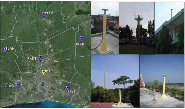
Fig. 1. General distribution of the CORS stations (left) and monumentation examples at the sites (right).

2.1. Data and Software

GNSS raw data in RINEX format came from seven CORS stations (Fig. 1). Six CORS stations belong to DOL network. These stations allowed us to compute daily network solutions and to generate the VRS data for NRTK offline processing. All DOL stations are equipped with identical high-grade Trimble NetR5 receivers. The other station belongs to the Department of Public Works and Town & Country Planning (DPT). This station was assigned as a (static) rover station. At this station, GNSS data was collected using high-grade Leica GRX 1200 Pro receiver. Dual-frequency phase and code observations have been collected above a 5-degree cut-off elevation with a sampling rate of 1 sec (DOL) and 5 sec (DPT), respectively. In addition to GNSS data, the study counted on several software applications as follows. The raw observations were processed using Leica Geo Office (LGO) commercial package. The DOL web application was used to generate and download the VRS observation data. Editing and quality checking was done using TEQC toolkit [11]. Finally, ionospheric activity representing various scenarios was extracted and selected using the Trimble GNSS Planning Online tool.

2.2. Date Selection

The data covered seven days: three in 2014 (DOY 108, 198, 303) and four in 2015 (DOY 041 to 044). The selection process had in mind to express the ionopheric activity through the total electron content (TEC) values. Thus, we selected four scenario levels: low (<40), medium (40-80), high (80-120), and extreme (>120) ionospheric activity. Figure 2 illustrates the ionospheric activity for these scenarios using Trimble’s GNSS planning online tool. Here, we should mention that high and extreme scenarios seem to include no scintillation event or plasma bubble even though such events occur very frequently in Thailand [12]. Since the equatorial plasma bubble analysis is not directly related to the topic of this work, we consider the abovementioned scenarios relevant for the aim of this study.

2.3. Data Processing

Fig. 2. Ionospheric activity during low, medium, high and extreme TEC scenarios.

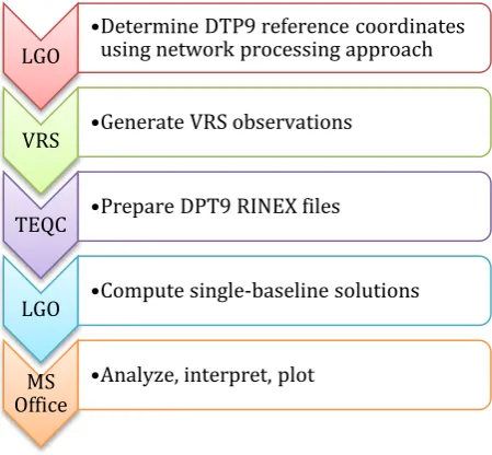
Fig. 3. Data processing workflow.

In the second step, we generated VRS observations as one-day correction data for all four individual test scenarios explained above. In the third step, we prepared the DPT9 observation files using TEQC toolkit. Each 24h RINEX file from DPT9 was split into short sessions of different lengths and number of epochs (10, 30, 60, 120, 180, 360, and 720 epochs). Since the sampling rate for DPT9 was 5 sec, the 720-epoch case corresponds to 1 hour of data. For the sub-hourly cases, we considered only the first file within the hour. This means a total number of 168 samples were computed each day (Table 1). In the fourth step, we produced NRTK solutions as 3D geocentric coordinates for all files. These solutions were computed as

LGO

•Determine DTP9 reference coordinates using network processing approach

VRS •Generate VRS observations

TEQC •Prepare DPT9 RINEX files

LGO •Compute single-baseline solutions

MS Office

single baseline between VRS and DPT9. The NRTK positions were exported to UTM coordinates for further analysis. In the final step, we analyzed, interpreted, and plotted the obtained results. They are presented in the following section.

Table 1. Number of epochs and session lengths at DPT9 station in various scenarios.

Epochs

per file Session length (seconds) Files per day Processed files

10 50 1728 24

30 150 576 24

60 300 288 24

120 600 144 24

180 900 96 24

360 1800 48 24

720 3600 24 24

Table 2. Discrepancies between average and daily network solutions at DPT9 station.

Station DOY Discrepancies [m]

dE dN dh

DPT9 14108 -0.001 -0.003 -0.020

14198 -0.001 -0.001 -0.005

14303 0.006 -0.000 0.000

15041 0.000 0.006 0.004

15042 -0.003 0.000 0.008

15043 -0.002 0.002 0.011

15044 0.001 -0.003 0.001

3.

Numerical Results and Discussions

3.1. Reference Coordinates

In order to assess the positioning performance, we produced the best possible coordinates for DPT9. Thus, seven days of 24-hour data at 30 sec sampling interval were processed in a network adjustment solution using LGO processing software. All DOL CORS stations were fixed and daily WGS84 coordinates were computed for DPT9. The coordinates were transformed to UTM projection and a seven-day average solution was computed. Table 2 presents the discrepancies between the daily and the average solution. The peak-to-peak discrepancies are within 1 cm in both horizontal directions and 3 cm in the vertical direction. The day with extreme TEC values showed the largest discrepancy in the vertical component.

3.2. Post-Processing with VRS Data

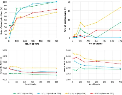
All VRS-based solutions were compared to the reference coordinates. In this study, we defined three main indicators to characterize the positioning performance: the rate of ambiguity fixing, the rate of position jumps, and the root mean square indicator. The rate of ambiguity fixing defines the percentage ratio between ambiguity fixed solutions and all data used in the processing. The rate of position jumps shows the percentage ratio of the ambiguity fixed solutions that fell outside the 5- and 10-cm error circle in the horizontal and vertical plane, respectively. RMSE values are computed in both horizontal and vertical directions using only the solutions with fixed ambiguity and no jumps. Figure 4 depicts the three performance indicators for different ionospheric activity scenarios.

TEC). Next, although the position jump rate is not correlated clearly with session length and ionospheric effects, the highest and lowest rates occur on intense and moderate TEC cases, respectively. Finally, RMSE indicator gradually decreases in both horizontal and vertical directions as the session length increases. While the differences in horizontal RMSE are not so significant, the vertical RMSE values show clear differences for different scenarios. The performance indicators demonstrate the importance of session length and the impact of residual ionospheric biases on the positioning results. Therefore, the user may be able to use DOL-VRS service for control survey. However, the user is advised to check various ionosphere or space weather monitoring services before going into the field for high-accuracy projects.

Fig. 4. Positioning performance indicators for different ionospheric activity scenarios: low (green), medium

(blue), high (yellow) and extreme (red).

3.3. Precision Test

Precision is a computed statistical quantity to describe the degree of repeatability between repeated measurements of the same quantity. It is a way to describe the quality of the data with respect to random errors. Precision is traditionally measured using the standard deviation and therefore is shown in the RMS error on the data collector screen [13].

solutions landed inside. Further specific investigations need to be carried out to better understand the reasons behind this result. Nevertheless, this test shows how high TEC influence significantly the solution distribution and repeatability.

Fig. 5. Horizontal scatter of the 720-epoch solutions for different TEC conditions.

Table 3. Statistical indicators for the precision test on various TEC conditions [units: meter].

Statistical

indicator Error component low medium TEC conditions high extreme

MAX dE 0.014 0.021 0.028 0.019

dN 0.006 0.012 0.045 0.017

MIN dE -0.001 0.000 -0.008 -0.002

dN -0.005 -0.006 -0.020 -0.013

Range dE 0.015 0.021 0.037 0.021

dN 0.010 0.018 0.064 0.030

RMSE dE 0.007 0.013 0.019 0.011

dN 0.017 0.019 0.032 0.026

Inside 2 cm diameter circle 22 20 4 12

Outside 2 cm diameter circle 0 4 9 6

No fix & position jumps 2 0 11 6

TOTAL 24 24 24 24

3.4. Accuracy test

Accuracy is a computed statistical quantity to describe the degree of closeness of a measured value of a quantity to its “true” value. Although the accuracy accounts for all types of errors, it is particularly related to the influence of systematic errors. Typically, the alignment to the truth is done by some method of post-processing observations of the GNSS station constrained by CORS data [13]. Therefore, we define the seven-day average reference solution computed in section 3.1 as our truth in this analysis.

landed inside DRMS circle, whereas 91.6% do no exit the 2-cm diameter circle. However, most of the short sessions and their VRS solutions fell outside the 2-cm testing circle indicating they do not reach the positioning specifications for high accuracy projects.

Fig. 6. Horizontal precision vs. accuracy.

Fig. 7. Vertical error distribution during each observation day.

Table 4. Vertical error statistics for the 720-epoch solutions.

TEC

conditions DOY MAX MIN Statistical indicator [m] Range AVG RMSE

low 14198 0.004 -0.035 0.039 -0.014 0.017

medium 15043 0.017 -0.049 0.066 -0.010 0.019

high 14303 0.030 -0.071 0.101 -0.014 0.032

3.5. Vertical component

NRTK positioning provides also information in the vertical direction. In this test, we examine the precision and reliability of the vertical component in a same manner as in the previous section. Figure 7 illustrates the 720-epoch vertical solutions for each observation day. It seems that all solutions show a negative bias of 1.0 to 2.1 cm. The peak-to-peak errors vary from 3.9 cm (low TEC) to 10.1 cm (high TEC). These variations may not be suitable for high-precision control survey. Generally, the RMS errors are between 1.7 and 3.2 cm. Table 4 summarizes the main statistics for the 720-epoch vertical solutions. Nevertheless, the results also indicate that higher precision may be achieved during quiet days. In addition, increased observation session length produces better precisions and is essential when elevations are determined using GNSS positioning.

4.

Conclusions

This study has aimed to provide an investigation on the feasibility of DOL-VRS service for establishing survey control. Thus, three performance indicators were defined: the rate of ambiguity fixing, the rate of position jumps, and the root mean square indicator. The numerical results revealed that reliable survey control depends on the session length and the residual ionospheric bias. For example, at least 180 observation epochs are needed on good ionospheric conditions. However, 720 epochs or more are needed if ionospheric activity increases. For shorter session lengths, there is a high probability not to be able to get an ambiguity-fixed solution or to get an incorrect ambiguity-fixed solution. The increase in ionospheric activity influences directly the spread of the solution in both horizontal and vertical directions. In this study, 60.4% of the solutions (58 out of 96) landed inside a 2-cm diameter circle, whereas 19.8% of the solutions (19 out of 96) landed outside the circle. The remaining 19.8% included no ambiguity-fixed solutions and/or position jumps. The best results were obtained on the day with low TEC values when all 720-epoch solutions felt inside the circle. In addition, VRS solutions exhibited an offset of about 0.7 cm with respect to a seven-day average network solution. On the other hand, the errors in the vertical direction for 720-epoch solutions displayed peak-to-peak variations of 3.9 cm (low TEC) to 10.1 cm (high TEC). These variations may be too large for certain high-precision control surveys. In addition, the RMS vertical errors were between 1.7 and 3.2 cm. Thus, we advice users to exert caution when using the service for high-precision control surveys. The user is advised to take average of multiple occupations on the same mark on different times of the same day or different days. The occupations should be separated in time to allow changes in the constellation geometry and ionospheric conditions. Furthermore, the user should also follow the updates from various space weather monitoring services before going into the field for high-accuracy projects. Such practice will enhance the productivity and reliability to establish high accuracy survey control.

Acknowledgements

This research was partially funded by the Chulalongkorn University Ratchadaphisek Somphot Endowment Grant GDNS 57-041-21-002. The first author would like to acknowledge support from the Department of Lands (DOL) and the Department of Public Works and Town & Country Planning (DPT) in completing his senior project.

References

[1] U. Vollath, A. Buecherl, H. Landau, C. Pagels, and B. Wagner, “Multi-base RTK positioning using

virtual reference stations,” in Proc. the 13th International Technical Meeting of the Satellite Division of The Institute of Navigation (ION GPS 2000), Salt Lake City, UT, 2000, pp. 123-131.

[2] H. Landau, U. Vollath, and X. Chen, “Virtual reference station systems,” Journal of Global Positioning Systems, vol. 1, no. 2, pp. 137-143, 2002.

[3] C. Rizos and C. Satirapod, “Contribution of GNSS CORS infrastructure to the mission of modern

[4] T. Charoenkalunyuta and C. Satirapod, “Accuracy assessment of real-time kinematic GPS surveying using the first Virtual Reference Station (VRS) network in Thailand: Initial test results,” Kasetsart Engineering Journal, vol. 23, no. 70, pp. 45-56, 2010.

[5] R. Attaviriyasuwon, T. Boonchuk, N. Leelaruji, and N. Hemmakorn, “Observation of ionospheric

height changes at Chumphon near the magnetic equator,” in Proc. 5th International Conference on Information, Communications and Signal Processing, Bangkok, Thailand, 2005, pp. 1169-1172.

[6] A. Gwal, S. Dubey, R. Wahi, and A. Feliziani, “Amplitude and phase scintillation study at Chiang Rai,

Thailand,” Advances in Space Research, vol. 38, no. 11, pp. 2361-2365, 2006.

[7] T. Musa, “Residual analysis of atmospheric delay in low latitude region using network-based GPS positioning,” Ph.D. thesis, School of Surveying and Spatial Information Systems, University of New South Wales, Australia, 2007.

[8] C.-O. Andrei, R. Chen, H. Kuusniemi, M. Hernandez-Pajares, J. M. Juan, and D. Salazar, “Ionosphere

effect mitigation for single-frequency precise point positioning,” in Proc. the 22nd International Technical Meeting of the Satellite Division (ION GNSS-2009), Savannah, GA, 2009, pp. 2508-2517.

[9] T. Charoenkalunyuta, C. Satirapod, H. K. Lee, and Y. S. Choi, “Performance of network-based RTK

GPS in low-latitude region: A case study in Thailand,” Engineering Journal, vol. 16, no. 5, pp. 96-103,

2012.

[10] T. Charoenkalunyuta and C. Satirapod, “Effect of Thai Ionospheric Maps (THIM) model on the

performance of network based RTK GPS in Thailand,” Survey Review, vol. 46, no. 334, pp. 1-6, 2014.

[11] L. H. Estey and C. M. Meertens, “TEQC: The multi-purpose toolkit for GPS/GLONASS data,” GPS

Solutions, vol. 3, no. 1, pp. 42-49, 1999.

[12] T. Tsujii, T. Fujiwara, T. Kubota, C. Satirapod, P. Supnithi, T. Tsugawa, and H. K. Lee,

“Measurement and simulation of equatorial ionospheric plasma bubbles to assess their impact on GNSS performance,” Journal of Korean Society of Surveying, Geodesy, Photogrammetry and Cartography, vol. 30, no. 6-2, pp. 517-523, 2012.

[13] National Geodetic Survey. (2011). Guidelines for Real Time GNSS Networks. [Online]. Available: