BMC 2006
Interpolant Learning and Reuse
in SAT-Based Model Checking
Joao Marques-Silva
1School of Electronics and Computer Science University of Southampton, Southampton, UK
Abstract
Bounded Model Checking (BMC) is one of the most paradigmatic practical appli-cations of Boolean Satisfiability (SAT). The utilization of SAT in model checking has allowed significant performance gains and, as a consequence, a large number of commercial verification tools now include SAT-based model checkers. Recent work has provided SAT-based BMC with completeness conditions, and this is generally referred to as unbounded model checking (UMC). Among the existing approaches for SAT-based UMC, the utilization of interpolants is among the most effective. Despite their success, interpolants have only been used for identifying a fixed point of the set of reachable states. This paper extends the utilization of interpolants in SAT-based model checking. This is achieved by observing that, under reason-able assumptions, interpolants can be reused, i.e. computed interpolants can be reused at later stages of the model checking process. The paper develops condi-tions for validity of interpolant reuse. In addition, the paper outlines a new fixed point condition, alternative to the existing interpolant-based fixed point condition. Preliminary practical experience on interpolant learning and reuse is reported.
Key words: Boolean Satisfiability, Bounded Model Checking, Interpolants.
1
Introduction
The utilization of Boolean Satisfiability (SAT) in Model Checking has been the subject of extensive research in recent years. The main result of this effort has been a number of fairly competitive incomplete and complete SAT-based model checking algorithms [3,4,5,20,21,26,27]. Moreover, SAT-based model checking has also been rapidly adopted by industry, and a number of vendors have included SAT-based Model Checking in their tools.
1 Email:[email protected]
This paper is electronically published in Electronic Notes in Theoretical Computer Science
The utilization of SAT in model checking was first proposed in the form of Bounded Model Checking (BMC) [3], where a counterexample is searched for increasing unfoldings of a finite state automaton. The original BMC work has been shown to be extremely useful for finding counter-examples but, unless the recurrence (or the reachability) diameter of the automaton is known [2], the BMC procedure is incomplete.
Different solutions have been proposed for ensuring the completeness of BMC [26,5,17,16,21], the most promising of which is arguably based on the utilization of interpolants [21].
This paper reviews the utilization of interpolants in SAT-based unbounded model checking and proposes the learning and reuse of computed interpolants with the purpose of allowing increased search pruning for subsequent calls to the SAT solver during the model checking process. The paper shows that different interpolants can be computed and used in different contexts. More-over, the paper outlines a fixed point condition alternative to the one proposed in‘[21].
We note that the main objectives of the paper are to investigate the con-ditions for interpolant reuse, and to propose an alternative interpolant-based fixed point condition. However, our experimental results suggest that inter-polant reuse may not yield improvements on industrial examples. A more effective implementation, as well as a more careful selection of which inter-polants to reuse, may yield more effective interpolant reuse.
The paper is organized as follows. The next section provides a necessarily brief perspective on SAT solvers and related concepts. Afterwards, Section 3
reviews SAT-based model checking, including bounded and unbounded model checking. Section 4develops conditions for reusing learnt interpolants. Initial practical experience is summarized in Section 5 and Section 6 concludes the paper.
2
Preliminaries
Propositional formulas are defined over finite sets of Boolean variables X =
{x1, x2, . . .}, W = {w1, w2, . . .}, X1, X2, etc., where each variable can be
as-signed value 1 (True) or 0 (False). In what follows propositional formulas
are represented by ψ1, ψ2, . . . . When relevant other subscripts can be used,
e.g. ψa, ψb, etc. For specific cases, letters and names representing predicates are also used for denoting the associated propositional formulas, examples include I, T, F, P, Q and Bmc. When referring to propositional formulas
propositional formula ¬ψ is used in an expression, it corresponds to ψ = 0. We consider model checking of LTL safety properties GψS. A finite state automaton M = (I, T, F) is assumed, where I is a predicate defined on state variables, T is the state transition relation, andF represents the failing prop-erty (i.e. F = ¬ψS), defined on state variables. Moreover, the utilization of predicates I, T or F assumes an underlying automaton M = (I, T, F). As mentioned above, for simplicity the propositional formulas associated with these predicates are represented with the same letters, I, T and F.
It will also be necessary to map propositional formulas from one set of vari-ables to another set of varivari-ables. The notationψ(Y /Yk) is used to denote that the propositional formulaψ, defined over the set of variablesY, is mapped into the set of variables Yk. Moreover, state variables are preferably represented as set Y, Yk when referring to the state variables in time step k. Boolean circuit variables are preferably represented as sets X orW, respectively Xk and Wk for variables in time step k, and finally auxiliary variables used in the CNF representation are preferably represented as sets W or Z.
2.1 Boolean Satisfiability Solvers
The remarkable evolution of Boolean Satisfiability (SAT) solvers over the last decade [19,23,14] has motivated the application of SAT in model checking. The most effective SAT solvers are based on backtrack search [9] and share a number of key techniques, including:
• Unit clause rule, also referred as Boolean constraint propagation, that con-sists of the identification of implied variable assignments [10].
• Clause learning, consisting of learning new clauses in presence of conflicts during the execution of backtrack search. A few techniques related with clause learning are the utilization of unique implication points (UIPs) [19], and non-chronological backtracking [19].
• Memory efficient lazy data structures [23].
• Adaptive branching heuristic, usually derived from the VSIDS heuristic [23].
• Utilization of search restarts [15], by using some completeness criterion.
Because modern backtrack search SAT solvers learn clauses, it is straightfor-ward to track all the learned clauses, and use these clauses for constructing a resolution refutation (or unsatisfiability proof) of the original formula [29].
2.2 SAT-Related Concepts
This subsection addresses a number of byproducts of modern SAT solvers, which are required for the utilization of interpolants in SAT-based model checking. For this purpose, we review proof traces, unsatisfiable cores and
unsatisfiability proofs.
instances, the original clauses and the learned clauses can be used for gener-ating a resolution-based unsatisfiability proof [29]. Modern SAT solvers can be instructed for generating a proof trace, which associates with each learned clause ω, all the clauses that explain the creation ofω [29].
Given a proof trace Γ, where the final traced clause is the empty clause⊥, we can identify, in linear time on the size of the proof trace, a subset of the original set of clauses which is itself unsatisfiable [29]. This subset is referred to as an unsatisfiable core.
Moreover, and given a proof trace Γ, generated by a SAT solver, it is possible to create a resolution-based unsatisfiability proof in time and size linear on the size of the proof trace.
Definition 2.1 [Unsatisfiability Proof [21]] A proof of unsatisfiability Π for a set of clauses ϕ is a directed acyclic graph (VΠ, EΠ), where VΠ is a set of
clauses, such that:
• For every ω∈VΠ, either
· ω∈ϕ, and ω is a root, or
· ω has two predecessors, ω1 and ω2, such that ω is the resolvent ofω1 and
ω2 (the variable v used for resolving ω1 with ω2 is referred to as the pivot
variable of the resolution step), and
• the empty clause ⊥is the unique leaf.
2.3 Craig Interpolants
Assume a propositional formula ψA(Y, X), defined over the sets of variables
Y and X, and a propositional formula ψB(Y, W), defined over the sets of variables Y and W. If ψA(Y, X)∧ψB(Y, W) is unsatisfiable, then there exists a propositional formula ψP(Y), defined over the set of variables Y, such that
ψA(Y, X)→ψP(Y) is a tautology andψB(Y, W)∧ψP(Y) is unsatisfiable. The propositional formula ψP(Y) is referred to as aninterpolant forψA(Y, X) and
ψB(Y, W) [8]. Recent work has shown that an interpolant can be constructed in linear time on the size of a resolution refutation ofψA(Y, X)∧ψB(Y, W) [25]. In what follows we outline McMillan’s interpolant construction [21], even though Pudl´ak’s construction [25] could also be considered. Regarding the propositional formulasψA(Y, X) andψB(Y, W), and associated CNF formulas, respectively ϕA(Y, X, U) and ϕB(Y, W, V), variables in set Y are referred to asglobalvariables, whereas variables in sets X andU arelocaltoϕA(Y, X, U), and the variables in sets W and V are local to ϕB(Y, W, V). Further, let g(ω) denote the literals corresponding to global variables in clause ω.
Definition 2.2 [Interpolant [21]] Let (ϕA, ϕB) be a pair of clause sets and let Π be a proof of unsatisfiability of ϕA∪ϕB, with leaf vertex⊥. For each vertex
ω ∈VΠ, let ψω be a Boolean formula, such that: • Ifω is a root then
Algorithm 1 Organization of BMC
BMC(M = (I, T, F),λ, ι, µ)
1 j ←0 2 k←λ
3 while k≤µ
4 doϕ ←Cnf(Bmckj(M), W)
5 if Sat(ϕ)
6 then return false Found counterexample
7 k ←k+ι
8 return true
· else ψω =True
• else, letω1, ω2 be the predecessors of ω and let v be their pivot variable
· if v is local toϕA, then ψω =ψω1 ∨ψω2,
· else ψω =ψω1 ∧ψω2
The Π-interpolant of (ϕA, ϕB), denoted Itp(Π, ϕA, ϕB) isψ⊥.
The interpolantItp(Π, ϕA, ϕB) has size linear on the size of the
unsatisfi-ability proof [25,21].
3
SAT-Based Model Checking
This section overviews the work on using SAT in model checking, emphasizing the initial work on Bounded Model Checking (BMC) and the more recent work on Unbounded Model Checking (UMC).
3.1 Bounded Model Checking
The generic Boolean formula associated with SAT-based BMC is the follow-ing [2,3,27]:
Bmck
j(M) =I(Y0)∧ ^
0≤i<k
T(Yi, Yi+1) !
∧ _
j≤i≤k
F(Yi)
!
(1)
This formula represents the unfolding of the state machine forktime steps, where I(Y0) represents the initial state, T(Yi, Yi+1) represents the transition
relation between states Yi and Yi+1, and F(Yi) represents the failing property
in time step i. Given the Boolean formula Bmck
j(M), it is straightforward to generate a CNF formula ϕ, by applying Tseitin’s [28] or the structure preserving [24] transformations, and by using additional auxiliary Boolean variables. This formula can then be evaluated by a SAT solver.
evidence has confirmed SAT-based BMC to be an extremely competitive tech-nique, that has been widely applied in industrial settings [2,7,12].
In order to describe the work on UMC and the reusing of interpolants, the following predicates are extensively used:
Unfoldsr(M) =I(Y−r)∧ ^
−r≤i<s
T(Yi, Yi+1) !
(2)
Trant
s(M) =
^
s≤i<t
T(Yi, Yi+1)
(3)
Propuv(M) = ^
u≤i<u+v
T(Yi, Yi+1) !
∧ _
u≤i≤u+v
F(Yi)
!
(4)
Hence, we can express the BMC formula in terms of these predicates:
BMCk
j(M) = Unfold j
0(M)∧Prop
j
k−j(M) = Unfold0
0(M)∧Tran
j
0(M)∧Prop
j
k−j(M) (5)
3.2 Unbounded Model Checking
A key difficulty with BMC is its inability for proving that there is no coun-terexample for a given safety property G ψS. Unless the recurrence (or the
Algorithm 2 UMC Algorithm
UMC(M = (I, T, F)) 1 k ←0
2 if Sat(I∧F)
3 then return false Counterexample found
4 while true
5 do status=CheckFixpoint(M, k)
6 if status = false
7 then return false Counterexample found
8 else if status = true
9 then return true Property proved
10 k ←k+ 1 Unfold further
3.3 Interpolant-Based Unbounded Model Checking
Recent work on SAT-based Unbounded Model Checking has addressed the utilization of interpolants [21], with quite promising experimental results. This section reviews McMillan’s interpolant-based UMC algorithm [21].
The definition of the BMC proposition formula is modified slightly with respect to (1):
Prefl(M) =I(Y−l)∧ V
−l≤i<0T(Yi, Yi+1)
= Unfold0
l(M) (6)
Suffk
j(M) =
V
0≤i<kT(Yi, Yi+1)
∧W
j≤i≤kF(Yi)
= Tranj0(M)∧Propj
k−j(M) (7)
Hence, the BMC formula becomes:
Bmck
j(M) =Pref1(M)∧Suffkj(M)
(8)
The above equation corresponds to the one proposed by McMillan [21], where the separation between prefix and suffix identifies the set of variables with respect to which interpolants are to be computed.
The SAT-based model checking algorithm can be organized into two main phases: a BMC loop, where the circuit is unfolded, and a fixed point check-ing step, that checks for the existence of a counterexample and where the existence of a fixed-point is tested. Observe that the second phase requires the iterative computation of interpolants until a fixed-point is reached or a true or (possibly) false counterexample is identified. The organization of the BMC loop is outlined in Algorithm 2, whereas the organization of fixed point checking step is outlined in Algorithm 3.
Algorithm 3 Fixed point identification in SAT-based UMC
CheckFixpoint(M = (I, T.F), k)
1 R ←I
2 while true
3 do M′ ←(R, T, F)
4 A←Cnf(Pref1(M′), W
1)
5 B ←Cnf(Suffk
0(M
′ ), W2)
6 (isSat,Γ)←Sat(A∪B)
7 if isSAT
8 then if R =I
9 then return false
10 else return abort
11 A∪B is unsat 12 Π←UnsatProof(Γ)
13 P ←Itp(Π, A, B)
14 R′ ←P(Y /Y
0)
15 C ←Cnf(¬R, W3)
16 D←Cnf(R′, W
4)
17 (isSat,Γ)←Sat(C∪D)
18 if notisSAT
19 then return true
20 R ←R∨R′
increasing k by values larger than 1 [18]. In addition, observe that the fixed point checking procedure consists of iterative computation of interpolants, where for iteration m the interpolant represents an abstraction of the reach-able states in m time steps [21]. At each iteration of the UMC fixed point checking procedure, the existence of a fixed-point is tested. The fixed-point is reached when the abstraction of the reachable states inm time steps contains only states already included in the abstractions of the reachable states in less than m time steps. Finally, observe that the algorithm sets j = 0, because interpolants are computed with respect to Y0.
4
Interpolant Learning and Reuse
This section develops conditions for reusing computed interpolants, and con-sists of two main parts. Conditions for interpolants representing over-approxi-mations of the set of reachable states, and conditions for interpolants repre-senting over-approximations of the set of states satisfying the failing property. We should note that the work on interpolant reuse is largely motivated by previous (and successful) work on clause reuse [27]. Clause reuse has been used extensively in BMC and is widely regarded as a key technique [27,12].
in-terpolants to be reused. Hence, the following definition is used extensively.
Definition 4.1 A Boolean formulaψN is said to beusablefor Boolean formula
ψB iff ψB →ψN.
Hence,ψN preserves satisfiability of the original formula and so we get the following straightforward result:
Proposition 4.2 LetψN be usable for ψB. Then ψB is satisfiable iff ψB∧ψN
is satisfiable.
In order to generalize the computation of interpolants, equation (5) is modified as follows:
Bmck
j(M) =Unfold k
0(M)∧Prop
k j(M) (9)
Observe that the new equation differs from (5) and (8). In equation (9) the failing property is checked for only in the last j time steps for an unfolding of
k+j time steps 2. (This approach is also used for example in [7,26,12].) For
simplicity we assume j = 0; generalization for j >0 is simple.
The standard interpolants used in [21] are referred to asdirect interpolants. It is also possible to compute reverse interpolants by exchanging the sets A
and B in the definition of interpolant. Direct interpolants are computed as described in McMillan’s work [21] (see also the previous section), but relaxing the 1 time step unfolding for A. For computing an interpolant after r time steps from I and t=k−r time steps from F, the propositional formulas for
A and B become:
A =Cnf(Unfoldr
0(M), W1)
(10)
B =Cnf(Trankk−t(M)∧Propk0(M), W2)
(11)
The interpolant computed with A and B above will be denoted Pr
t. It is also possible to compute an interpolant by replacing I with another interpolant
Pu v:
A=Cnf(Pvu(Y0)∧Tranr0(M), W1)
(12)
B =Cnf(Trank
k−t(M)∧Prop k
0(M), W2)
(13)
And the new interpolant is denoted Pu+r t . Consequently, Pr
t, with r, t≥ 0, denotes the direct interpolant computed with a (possibly virtual) unfolding of r time steps from the initial state, and
t time steps until the failing property is checked for. Hence, Pr
t represents an
over-approximationof the set of states reachable inrtime steps and an under-approximation of the set of states which do not satisfy the failing property in
t time steps.
Reverse interpolants are computed by interchanging the definitions of A
andBin (10) and (11), and will be denoted byQr
the reverse interpolant computed with an unfolding of r time steps from the initial state, and (possibly virtual) t time steps until the failing property is checked for. Hence, Qr
t represents anunder-approximation of the set of states that are not reachable inr time steps and anover-approximation of the set of states which satisfy the failing property in t time steps. From (10) and (11) we obtain:
A=Cnf(Trank
k−t(M)∧Prop k
0(M), W3)
(14)
B =Cnf(Unfoldr
0(M), W4)
(15)
The interpolant computed with A and B above will be denoted Qr
t. It is also possible to compute an interpolant by replacing F with another interpolant
Qu v:
A=Cnf(Trank
k−t(M)∧Q u v(Yk)) (16)
B =Cnf(Unfoldr
0(M), W4)
(17)
And the new interpolant is denoted Qr t+v.
Given the definitions of direct and reverse interpolants, we can now estab-lish conditions for interpolant reuse in SAT-based model checking.
Theorem 4.3 Let Bmck
j(M) be given by (9), and direct interpolants Ptr be
computed with (10) and (11). Then the following holds:
(i) Pr
t(Yr) is usable for Bmc k
j(M), with t≥0 and 0≤r ≤k. (ii) ¬Pr
t(Yk−t) is usable for Bmc k
j(M), with r ≥0 and 0≤t ≤k.
Proof.
(i) If Bmckj(M) is satisfiable, then Unfoldr0(M), with r ≤ k is also
satis-fiable and Yr represents a state reachable in r time steps. By definition,
Pr
t(Yr) represents an over-approximation of the states reachable inrtime steps. Hence, Pr
t(Yr) holds for any assignment to the variables inYr rep-resenting a state reachable in r time steps. Thus, Bmck
j(M) → Ptr(Yr), with r ≤ k. By definition, Pr
t(Yr) is usable for Bmc k
j(M), with r ≤ k. Observe that there is no upper bound on the value of t.
(ii) Observe that Pr
t(Yk−t) represents an under-approximation of the states which do not satisfy the failing property inttime steps. Hence,Pr
t(Yk−t)→
¬Bmck
j(M) with t ≤k. Consequently, Bmc k
j(M)→ ¬Ptr(Yk−t). By def-inition, Pr
t(Yk−t) is usable for Bmc k
j(M), witht ≤k. Observe that there is no upper bound on the value of r.
2
Theorem 4.4 Let Bmck
j(M) be given by (9), and reverse interpolants Qrt be
computed with (14) and (15). Then the following holds:
(i) Qr
t(Yk−t) is usable for Bmc k
j(M), with r≥0 and 0≤t≤k. (ii) ¬Qr
t(Yr) is usable for Bmc k
Proof. The proof is similar to the proof for Theorem4.3.
(i) If Bmckj(M) is satisfiable, then Trankk−t(M)∧Propkk(M), with t ≤ k
is also satisfiable and Yk−t represents a state that satisfies the failing property in t time steps. By definition, Qr
t(Yk−t) represents an over-approximation of the states that satisfy the failing property in t time steps. Thus, Bmck
j(M)→Qrt(Yk−t), with t≤k. By definition, Qrt(Yk−t) is usable forBmckj(M), witht≤k. Observe that there is no upper bound
on the value of r. (ii) Observe thatQr
t(Yr) represents an under-approximation of the states that are unreachable r in time steps. Hence, Qr
t(Yr) → ¬Bmc k
j(M), with
r ≤ k. Consequently, Bmckj(M) → ¬Qrt(Yr). By definition, Qrt(Yr) is
usable for Bmck
j(M), with r≤k. Observe that there is no upper bound on the value of t.
2
Remark 4.5 Even though we describe the most general setting for learning and reusing interpolants, the specific interpolants computed in the standard interpolant-based fixed point condition [21] are also usable according to the conditions of Theorems 4.3 and 4.4. Hence, interpolant reuse can be readily integrated in a standard interpolant-based UMC flow.
Remark 4.6 The conditions of Theorems 4.3 and 4.4 can be used in any
BMC/UMC setting, independently of whether a fixed point is used and whether it is based on interpolants.
Remark 4.7 It is straightforward to conclude that reverse interpolants can be used for developing a fixed point condition alternative to the one of [21]. Algorithm3can easily be adapted for using reverse interpolants, computed one time step from the time step at which the property is checked for. Similarly to image computation approaches in BDD-based symbolic model checking, the advantages of this alternative fixed point condition are expected to depend on the actual automaton.
5
Experimental Results
Instance w/o interpolants w/ interpolants
6-bit counter 1.51 5.29
7-bit counter 16.38 61.03
8-bit counter 236.90 784.81
I1 7.08 7.11
I2 31.36 36.96
I3 38.36 60.60
I4 52.45 58.25
[image:12.612.171.436.22.242.2]I5 150.54 157.81
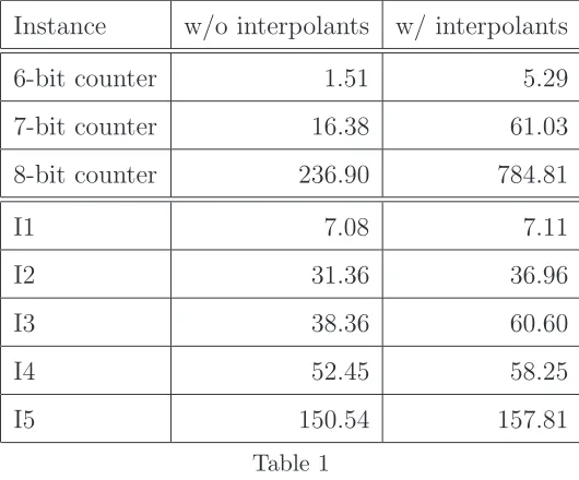
Table 1
Results with and without interpolant reuse
time step and reused in the last time step. As a result, reused interpolants serve for preventing sets of unwanted states to be reached.
Table 1 shows preliminary results from interpolant reuse. The first set of instances represent standard counters, for which counterexample exists. The second set of instances represent industrial problem instances, for which a counterexample also exists. As can be concluded, the utilization of inter-polants does not yield improvements to the run times. For the first set of (ar-tificial) examples the results are worse than for the second set of (industrial) examples. As mentioned above, the setup for the utilization of interpolants is certainly not the most adequate. We considered a simple BMC loop, where interpolants are solely used for search pruning purposes. The reuse of in-terpolants in a UMC setting is expected to provide more competitive results, since the interpolants have be computed for checking the fixed point condition.
6
Conclusions and Future Work
This paper develops conditions for learning and reusing of interpolants in SAT-based model checking. Computed interpolants can be used for requiring states from a set of states or for preventing states from a set of states. Besides interpolant reuse, an alternative fixed-point condition is also proposed, based on reverse (as opposed to direct) interpolants.
A few drawbacks of the current implementation have been identified. Ex-amples include the lack of structure sharing between different interpolants, and the fact that interpolants were computed solely for interpolant reuse and not for checking the existence of a fixed point. Integration of these improvements is expected to yield more promising results for interpolant reuse.
Acknowledgments
This work has been partially supported by European project IST-033709 VER-TIGO.
References
[1] P. A. Abdulla, P. Bjesse, and N. E´en. Symbolic reachability analysis based on SAT solvers. In International Conference on Tools and Algorithms for the Construction and Analysis of Systems, 2000.
[2] A. Biere, A. Cimatti, E. Clarke, O. Strichman, and Y. Zhu. Advances in Computers, chapter Bounded Model Checking. Academic Press, 2003.
[3] A. Biere, A. Cimatti, E. Clarke, and Y. Zhu. Symbolic model checking without BDDs. In International Conference on Tools and Algorithms for the Construction and Analysis of Systems, pages 193–207, March 1999.
[4] P. Bjesse and K. Claesen. SAT-based verification without state space traversal. In International Conference on Formal Methods in Computer-Aided Design, 2000.
[5] P. Chauhan, E. Clarke, J. Kukula, S. Sapra, H. Veith, and D. Wang. Automated abstraction refinement for model checking large state spaces using SAT based conflict analysis. InInternational Conference on Formal Methods in Computer-Aided Design, 2002.
[6] E. M. Clarke, O. Grumberg, and A. Peled. Model Checking. MIT Press, 1999.
[7] F. Copty, L. Fix, R. Fraer, E. Giunchiglia, G. Kamhi, A. Tacchella, and M. Y. Vardi. Benefits of bounded model checking at an industrial setting. In International Conference on Computer-Aided Verification, 2001.
[8] W. Craig. Linear reasoning: A new form of the Herbrand-Gentzen theorem.
Journal of Symbolic Logic, 22(3):250–268, 1957.
[9] M. Davis, G. Logemann, and D. Loveland. A machine program for theorem-proving. Communications of the Association for Computing Machinery, 5:394– 397, July 1962.
[10] M. Davis and H. Putnam. A computing procedure for quantification theory.
[11] N. Een and N. Sorensson. An extensible SAT solver. In Sixth International Conference on Theory and Applications of Satisfiability Testing, May 2003.
[12] N. Een and N. Sorensson. Temporal induction by incremental SAT solving. In
Workshop on Bounded Model Checking, volume 89 of ENTCS, 2003.
[13] M. Glusman, G. Kamhi, S. Mador-Haim, R. Fraer, and M. Vardi. Multiple-counterexample guided iterative abstraction refinement. In International Conference on Tools and Algorithms for the Construction and Analysis of Systems, April 2003.
[14] E. Goldberg and Y. Novikov. BerkMin: a fast and robust SAT-solver. InDesign, Automation and Test in Europe Conference, pages 142–149, March 2002.
[15] C. P. Gomes, B. Selman, and H. Kautz. Boosting combinatorial search through randomization. In National Conference on Artificial Intelligence, pages 431– 437, July 1998.
[16] A. Gupta, M. Ganai, Z. Yang, and P. Ashar. Iterative abstraction using SAT-based BMC with proof analysis. In International Conference on Computer-Aided Design, November 2003.
[17] H.-J. Kang and I.-C. Park. SAT-based unbounded symbolic model checking. In Design Automation Conference, pages 840–843, June 2003.
[18] J. P. Marques-Silva. Improvements to the implementation of interpolant-based model checking. In Advanced Research Working Conference on Correct Hardware Design and Verification Methods, October 2005.
[19] J. P. Marques-Silva and K. A. Sakallah. GRASP: A new search algorithm for satisfiability. In International Conference on Computer-Aided Design, pages 220–227, November 1996.
[20] K. L. McMillan. Applying SAT methods in unbounded symbolic model checking. In International Conference on Computer-Aided Verification, July 2002.
[21] K. L. McMillan. Interpolation and SAT-based model checking. InInternational Conference on Computer-Aided Verification, 2003.
[22] K. L. McMillan and N. Amla. Automatic abstraction without counterexamples. InInternational Conference on Tools and Algorithms for the Construction and Analysis of Systems, April 2003.
[23] M. Moskewicz, C. Madigan, Y. Zhao, L. Zhang, and S. Malik. Engineering an efficient SAT solver. In Design Automation Conference, pages 530–535, June 2001.
[24] D. A. Plaisted and S. Greenbaum. A structure-preserving clause form translation. Journal of Symbolic Computation, 2(3):293–304, September 1986.
[26] M. Sheeran, S. Singh, and G. Stalmarck. Checking safety properties using induction and a SAT solver. In International Conference on Formal Methods in Computer-Aided Design, 2000.
[27] O. Strichman. Tuning SAT checkers for bounded model checking. In
International Conference on Computer-Aided Verification, July 2000.
[28] G. S. Tseitin. On the complexity of derivation in propositional calculus. Studies in Constructive Mathematics and Mathematical Logic, Part II, pages 115–125, 1968.