Variable Discrimination of Crossover Versus Mutation
Using Parameterized Modular Structure
Rob Mills
Electronics and Computer Science University of Southampton Southampton, SO17 1BJ, UK
+44 23 8059 8703
[email protected]
Richard A. Watson
Electronics and Computer ScienceUniversity of Southampton Southampton, SO17 1BJ, UK
+44 23 8059 2690
[email protected]
ABSTRACT
Recent work has provided functions that can be used to prove a principled distinction between the capabilities of mutation-based and crossover-based algorithms. However, prior functions are isolated problem instances that do not provide much intuition about the space of possible functions that is relevant to this distinction or the characteristics of the problem class that affect the relative success of these operators. Modularity is a ubiquitous and intuitive concept in design, engineering and optimisation, and can be used to produce functions that discriminate the ability of crossover from mutation. In this paper, we present a new approach to representing modular problems, which parameterizes the amount of modular structure that is present in the epistatic dependencies of the problem. This adjustable level of modularity can be used to give rise to tuneable discrimination of the ability of genetic algorithms with crossover versus mutation-only algorithms.
Categories and Subject Descriptors
I.2.8 [Artificial Inteligence]: Problem Solving, Control Methods, and Search – heuristic methods.
General Terms
Algorithms, Performance, Reliability, Theory.
Keywords
Mutation, crossover, modularity, building block hypothesis, nearly decomposable systems.
1.
INTRODUCTION
We observe modular structures in an extensive variety of locations, from phenotypic development in biological systems [29] to human-engineered systems where, for example, the concept of decomposability is one of the key assumptions required for cell library utilisation in ASIC design [26]. When considering problems in evolutionary computation, the concept
that one portion of a system can be solved in partial or full isolation of other portions of the system is both simple and intuitive, and forms the basis for the building-block hypothesis (BBH) [12][13][8][20]. However, identifying problems which exhibit modular properties of the right kind to allow solutions to be more easily accessible to algorithms which exploit these modular properties is not straightforward [6].
The building block hypothesis is an early proposal to explain why the genetic algorithm (GA) is successful when it is [12][8]. It proposes that crossover recombines short high-fitness schemata to produce even fitter genotypes, offering a search capacity unavailable to other methods such as mutation hill climbing. In this paper we use the intuition of the BBH to construct a function that discriminates the capabilities of crossover and mutation methods. Of course, the discrimination of crossover and mutation in GAs has a long and controversial history [6][7][27][15][1][28]. Recently there have been some successes in showing principled distinctions between the ability of mutation and crossover: some are not based on building blocks [24][14], whereas some do utilise a building-block structure [30][31][34]. The most recent of these [34] uses a simple single-level building-block function to discriminate the ability of mutation and crossover in much the same way as that described by the BBH. However, all of this work addresses single problem instances which cannot be tuned to control the amount of modularity in the problem. Here we define a problem with parameterised structural modularity to investigate how this affects the discrimination between mutation and crossover. It is not the aim of this paper to uphold the BBH or untangle the issues involved in its controversial history – that requires a more direct and formal approach [34]. Our objective is to investigate how the distinction between mutation and crossover is sensitive to how structured the modularity of a problem is. This is performed using a simple building block function with a variable amount of modularity. That is, we investigate a problem that is adjustable from one extreme of no modularity at all to a problem that exhibits modular interdependency [2] (with very neat and clean modular structure), and parameterise the space in between these extremes.
In this paper, we introduce a new problem which exhibits modular interdependency [2]. We use an intuitive representation for this problem which permits us to vary the clarity of modular structures over a number of dimensions. The case where the modularity is clean and neat is sufficient to discriminate between mutation and crossover in a principled manner. Furthermore, our method for varying the structural modularity is described and investigated,
Permission to make digital or hard copies of all or part of this work for personal or classroom use is granted without fee provided that copies are not made or distributed for profit or commercial advantage and that copies bear this notice and the full citation on the first page. To copy otherwise, or republish, to post on servers or to redistribute to lists, requires prior specific permission and/or a fee.
and we find that the discrimination varies as the structural modularity is adjusted across the range we define.
There are many different ways that a problem could be tuned to show a variable amount of difficulty for mutation (e.g. [16]), and many parameters may be involved in the definition of functions that might influence the discrimination of mutation and crossover algorithms [22][4]. If nothing else, one could vary the size of a problem or the width of fitness valleys incorporated in the problem (e.g. [14][31]). One notable factor influencing the effectiveness of crossover is the tightness of the genetic linkage (the defining length of building blocks) [12][9]. But none of these methods directly addresses a variable amount of modularity in a simple tight-linkage building-block problem. Since the amount of modularity is parameterized in our new problem, we gain an understanding about properties which allow a GA using crossover to perform qualitatively differently when compared with a mutation-only algorithm. The level of discrimination changes as the structural modularity is varied, which indicates when crossover becomes necessary to solve the problem.
The key to making our problem variably modular is very simple. We define the fitness of a genotype using a sum of weighted pairwise interactions between the problem variables. For the highly modular case strong interaction weights within blocks are cleanly divided from the weak interactions that are between blocks. In the non-modular case these weights are randomised so that weights inside modules are not different on average from weights between modules. A partially modular problem is defined by partially randomising the weights of the modular case. It should be noted that problems built of pairwise interactions, or only order-2 dependencies, can often be easy to solve [16][8]. But this depends on how the interactions are organised. When dependencies are structured, pairwise dependencies can ‘act in concert’ to create local optima with significant Hamming distances between them [2][33]. Varying this structure is sufficient to vary the problem difficulty, and more importantly vary the discrimination between the abilities of crossover and mutation. Note that although the internal and external modular dependencies are parameterized in the NKC landscape [17], this has not been shown to discriminate the abilities of crossover and mutation even when the modularity is as strong as possible [34].
The remaining sections of this paper are organised as follows: section 2 introduces the new representation and discusses expected behaviour of crossover and mutation on this problem class; in section 3 we provide some experimental results. Section 4 discusses the consequences of the results in section 3. Section 5 concludes.
2.
PARAMETERIZING STRUCTURAL
MODULARITY: THE VSMP
2.1
Introduction
In order to address our goal, we require a problem which exhibits the type of modular properties which discriminate between the capabilities of crossover and mutation. We would also like to parameterise these modular properties, and in this section we present a problem class which satisfies these objectives.
A modular problem without inter-module interdependencies is defined as separable [32]. Simon calls particular types of non-separable modular systems ‘nearly decomposable’ [25]. Watson
refines this definition to describe problems which are decomposable but not separable as exhibiting ‘modular interdependency’ [32][2]. We do not wish to restrict our scope to separable problems, so we allow inter-module dependencies in our problem. We introduce a method which is intended to describe problems which exhibit modular interdependency. Note that in principle, systems which exhibit modular interdependency may still be easy for crossover [32]. Note also that in a function built only of pair-wise dependencies, inter-module dependencies must be weak when compared with intra-module dependencies since the strong internal dependencies are what define the module. For the sake of clarity, we shall refer to intra-module and inter-module dependencies as internal and external dependencies respectively.
In this section we introduce the problem representation and discuss the impact upon mutation and crossover variation operators. When talking about mutation, we are referring specifically to incremental processes such as point mutation, and not sequence based mutations (e.g. inversion, translocation). In this section crossover refers to variation operators which recombine genetic material from two parents. In the following chapter, we perform simulated experiments on the problem with specific algorithms in each of these classes. These specific choices are defined fully when relevant.
We approach the definition of our parameterized modular problem by initially considering a very simple non-modular problem and subsequently incorporating modular structure. We defer the introduction of components required for parameterization until the basic modular function is established.
2.2
A Simple Non-Modular Problem
We take a problem of N binary variables, giving N2 pair-wise interactions. Each pair of variables (i, j) contributes to the overall fitness of a candidate solution provided that the pair have the same value. More generally, a pair may contribute to the overall fitness of a candidate solution provided that the pair satisfies some arbitrary Boolean subfunction, and this may be a different function for different pairs. However in this paper we address only the subfunction of equality (if-and-only-if) because its effects are easy to understand. This subfunction causes dependencies to act in concert, which can produce wide fitness saddles [30]. If we assume that all pairs are of equal importance, then the overall fitness of a candidate is given by Eq. 1.
(
)
∑∑
−(
)
= −
=
−
=
↔
1
0 1
0 1
1 0
,
,...,
N
i N
j
j i
N
w
x
x
x
x
x
F
Eq. 1.Although this problem has a large number of interdependencies (N2), it contains no structure. The function has only two optima in its landscape, each of equal fitness. Paths of monotonically increasing fitness exist which lead to each of these solutions and thus either would be easily discovered by a mutation-only process.
2.3
A Simple Modular Problem
the weight of interactions within a module, and wE for the strength of interactions between modules.
These shall be represented in an N-by-N matrix, called the Pairwise Weight Matrix (PWM). The overall fitness of a candidate is now given by Eq. 2:
(
)
∑∑
−(
)
= −
=
−
=
↔
1
0 1
0 1
1 0
,
,...,
N
i N
j
j i ij
N
w
x
x
x
x
x
F
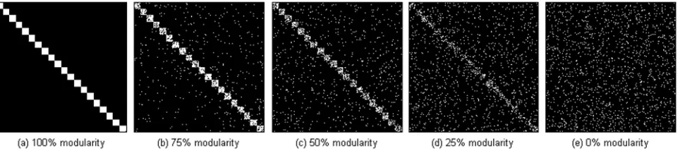
Eq. 2.Using just two weight classes keeps our problem formation simple, and yet allows us to represent a number of modules within which the internal dependencies are far more important than those outside of the module. Arranging blocks of strong internal dependencies close to the leading diagonal of the PWM introduces a number of modules, each containing variables that have tight physical linkage on the genome. The problem we define has Z modules each of k binary variables, giving an overall problem size of N=Z·k. Eq. 3 describes more specifically the positioning of the weights to generate the required modules (see also Figure 2 (a)):
. / /
, ,
otherwise k j k i if wE wI
wij =
= Eq. 3.
The PWM together with the IFF pairwise subfunction characterize the parameterised problem which we call the variable structural modularity problem (VSMP). A 20-module example is given in 2.4. Note that it is not required that all modules are of equal size, but this simplification is suitable for our purposes.
Using a matrix of pairwise dependencies in conjunction with a pairwise subfunction has been presented in [33] which shows a version of the Hierarchical-IFF function built from pairwise dependencies. Here we address a more straight-forward single-level of modularity rather than hierarchical modularity. This concept of modularity represented by a pairwise dependency matrix with high values grouped along the diagonal in this manner is both natural and intuitive [25][18][23][10][11][21][34]. The strong internal dependencies provide a selective gradient towards all variables within a module agreeing, resulting in two equally fit optima which are equally easy to find. As such we expect the probability of finding each optimum of a module to be on average 0.5 when considered in isolation.1 However, the overall fitness of a genotype will be increased in proportion to how many pairs of modules ‘agree’ in how they are solved, i.e. if either both are at the all-0’s solution or both are at the all-1’s solution. This is because these configurations also confer the fitness contribution bonuses from the external dependencies. This means that the optimal solution to a module is not independent of context, but is nevertheless always one of only two possibilities, all-0 or all-1. This modular interdependency [2] requires a search method which
1
The presence of external dependencies means that there is a bias towards one optimum or the other in all blocks in accordance with the majority of values for variables outside the block. This bias can be seen as a skewing of the landscape within a module, such that in the context of the rest of a genotype, one solution will be fitter than the other. Thus if external dependencies are too strong, one of the two internal local optima can be lost when the genotype as a whole has significantly more ones than zeros or vice versa.
explores combinations of blocks in order to find optimal solutions – and this is exactly the mechanism that crossover provides.
2.4
An example function
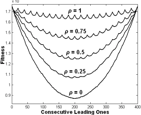
We consider a specific landscape for the function described by Eqs 2 & 3, for N=400, Z=k=20, wI=200 and wE=1. Figure 1 shows a particular cross-section of the fitness landscape defined by this function. The curve shows the fitness of each genotype G from G=0N to G=1N and all genotypes G=1i0N-i in between. i.e.
[image:3.595.311.541.215.403.2]00000…, 10000…, 11000…, 11100… etc.
Figure 1. A cross section through the fitness landscape for the clean VSM problem with N=400, Z=k=20, wI=200, wE=1.
This slice through the fitness landscape shows 21 different optima at 11 different fitness values. In the entire landscape there are 2Z (10
6
) local optima: the sparseness of optima is 2Z/2N =1/2k (1 in
106). However, each of the 21 shown in Figure 1 have ZCR,
equivalents, where R is the number blocks solved with all 1’s at that point in the section. Although this cross-section only shows
N+1 of a possible 2N genotypes, all of the local optima in the
landscape are either on or have an equivalent on the cross-section, and so it still provides valuable insight into the formation of the landscape.
We choose a problem that is large enough to discriminate methods using crossover from those only using mutation. Setting
Z=k maximises the trade-off between the width of fitness valleys
separating neighbouring local optima and the total number of local optima in the problem. The absolute values of wE and wI are not significant, however the ratio of these two weights is important. As the internal and external weights tend to equality, the local optima disappear, and in the limit of wI=wE the function becomes the simple problem of maximising the majority of 0’s or 1’s (as discussed previously in 2.2). In the other extreme, when
wE/wI tends to 0, all modules become separable and all 2Z local optima have equal fitness. The class of optima that have 19 solved modules of one type (either all-0s or all-1s) and 1 solved module of the other type is the last to appear with increasing
wI:wE, and this occurs at a ratio of 19:1. We choose wI:wE to be
Figure 2. Pairwise Weight Matrices for N=400, Z=k=20, wI=200, wE=1 for a range of modularity levels. Note that the dark region indicates the value is wE, which in general is non-zero
2.5
Performance Predictions for Mutation
and Crossover
So why is this problem class theoretically interesting? Our motivation is that this function will provide a basis to discriminate between an algorithm employing crossover and one using only mutation. Here we discuss what properties make this the case for the problem described in 2.3.
Let us consider a single module in isolation. As discussed in 2.3 equally fit optima exist at all-0’s and at all-1’s, and each are equally easy to discover. As such we expect the probability of finding each optimum to be 0.5 when considered in isolation. As identified in 2.4, there are 2Z local optima, only two of which are
global optima. If we set wE=0, all optima become global. Hence, we should expect each of the 2Z optima to be found by mutation with equal probability, and thus expect mutation to be sufficient to reliably solve the problem. If, however, we were after one of only two particular local optima, we should expect a mutation-only algorithm to succeed with a probability of mutation-only 2-(Z-1). With large Z this becomes infeasible. As noted in 2.3, when wE is non-zero, if there is an unequal number of 0’s and 1’s across the genotype, then a bias exists within each block towards the block optima which agrees with the majority. Although this makes the probability of finding a global optima slightly better than 2-(Z-1) for a mutation-only method, the presence of large numbers of local optima ensures that it remains very low.
For an algorithm employing both mutation and crossover, the story is rather different. Each module is easy to solve, and so we expect each individual to find one of the two solutions for each of the modules. Although the variable values within each of these modules will match other values in the same module, not all of the modules will agree with other modules, and some of the fitness contributions from external weights will not be obtained: the individual is at a local optimum. However, across a population we expect that different individuals will discover different solutions to each module. Even with a small population all of the module-solutions should be available in at least one of the individuals before long. The strong internal dependencies have been the main selective guide so far, and mutation is a sufficient operator in this stage. Now an algorithm which uses crossover should be able to compose combinations of these module solutions. The weaker external weights provide some gradient information that selection can act upon, preferring candidates closer to a global optimum. This process will only happen if the multiple solutions to each module are discovered by the population (and not subsequently lost prematurely through
competition), and if the module solutions are preserved by the crossover mechanism. The former condition requires a) crossover not to be too disruptive and allow mutation to discover all module solutions, and b) diversity maintenance to help preserve each module solution somewhere within the population. The latter condition also has two requirements. Firstly, modules must have tight linkage ( short defining length). Secondly, the crossover mechanism must preserve linkage, which is a feature of one or two point crossover for instance, but not uniform crossover. Thus our VSMP with clean modularity should properly discriminate between crossover and mutation based algorithms in a principled manner. The problem is difficult not because solving individual blocks is difficult, but because finding the correct combination of block solutions is difficult [34].
2.6
Parameterising the amount of Modularity
It still seems somewhat restricted to only consider such neatly formed modular problems, even if they do exhibit modular interdependency. We can modify the problem in a number of ways which will vary the level of modularity that is present whilst still maintaining the essence of the ideal modular problem, at least for a portion of the variation scale. These include:
• Variation in the values of weights in the PWM
• Variation of position of the classes of weights in the PWM
• Variation of the pairwise sub-functions
Varying the problem using these different methods can modify the properties in significantly dissimilar ways; this is discussed further in section 4. However in this paper we investigate a single method of adjusting the modularity present: to modify the positions of the classes of weights in the PWM. Note that varying the correspondence of the epistatic modularity to the genetic map (i.e. varying the tightness of the genetic linkage) is another way to vary the ease with which a GA will find good solutions. However the correspondence of epistatic modularity with the genetic map is a different issue from varying the modularity of the problem per
se, as addressed here: our method of varying the modularity in the
problem is not equivalent to shuffling the genetic map as it is not guaranteed that any amount of rearranging the loci would recover perfect modularity.
In order to explain the scale we use for structural modularity, we first consider the limits before deriving equations to describe the distribution of weights for the parameterised case.
of modularity, we start to see external weights where internal weights once were, and vice versa. We label the region where internal weights exist in the neat VSMP as rI, and similarly use rE for the region containing external weights. Figure 2(b)-(e) shows PWMs for a range of levels of structural modularity.
Regardless of the level of modularity, the number of wI weights and wE weights remains constant so as not to change the total amount of epistasis in the problem. Thus, the proportions of the total number of weights that have the values wI and wE are 1/Z and (Z-1)/Z respectively.
In the neat VSMP (i.e. at structural modularity=1), we see the proportion of wI weights in region rI is 1, and correspondingly find a proportion of 0 wI weights in rE. We define the other end of the scale to have wI weights randomly distributed, and as such expect to find a density of 1/Z in both regions rI and rE. For intermediate points in this scale of structural modularity, we linearly interpolate the proportion of wI weights in rI from 1 to 1/Z, and the proportion of wI weights in rE from 0 to 1/Z. Specifically, for a level of modularity , the proportion of weights in rI that have the value wI is 1/Z+ (1-1/Z), and the proportion of weights in rE that have the value wI is 1/Z- (1/Z).
Figure 3. A cross section through the fitness landscapes for the VSM problem for N=400, Z=k=20, wI=200, wE=1, with varying degrees of modularity, . As the modularity increases,
so does the height and number of local optima in the problem
Figure 3 shows the same cross-section through the genotype space as Figure 1: all of the genotypes G=1i0(N-i), for instances with varying levels of modularity, from randomly distributed wI weights ( =0) to neat structural modularity ( =1) in increments of 0.25 (see also Figure 2 (b)-(e)). For the case of =0, we see the function has no local optima and there are monotonically increasing fitness gradients leading to each global optimum. This is qualitatively comparable to the landscape we would find when
wI=wE, as discussed earlier (Eq.1). As we increase the structural
modularity towards =1, we see the landscape approach that shown in Figure 1 (this line is repeated in Figure 3 for comparison) with local optima increasing in number and height. Note that as all subfunctions are IFF the global optima will always be at all-1’s and all-0’s, regardless of the level of structural modularity.
2.6.1
Predictions for behaviour on variable problem
In section 2.5 we discussed the expected discrimination in behaviours of mutation and crossover based algorithms on the ideal modular problem. Here we discuss the expected behaviour of these two variation methods for the parameterised case. For =0, randomly distributed weights, we observe in Figure 2 (e) that no modular structure exists in the problem. One important consequence of this is that no local optima remain (see =0 line in Figure 3). In order to understand why the structure has been removed, we can take into account a subset of the variables in region rI in the PWM, of size Z by k. We call the average weight of this subset wIeff, and the average weight of the externaldependencies to these variables as wEeff. At this value of , We
expect wIeff and wEeff to be the same. That is, the dependencies
which defined the modules in the neatly modular problem no longer have any structure to qualify as a module.
This dissection of the problem properties for the case of = 0 allows us to confidently predict that this problem instance will not discriminate between mutation and crossover. As no local optima exist, a mutation-only method is sufficient for the reliable discovery of one of the global optima and no advantage will be seen when also using crossover.
For intermediate values of structural modularity, 0 < < 1, we observe that the integrity of the modular structures increases (see Figure 2 (b)-(d)), and the abundance of local optima increases (see Figure 3) with increasing . Again, we can consider the average fitness of the Z by k subset to understand why these changes occur. The average internal weight, wIeff, increases with
, whereas wEeff will decline. This has the effect of strengthening
modular structures which improves the fitness bonus attained when all variables agree. When is large enough that this fitness bonus is greater than the sum of the external agreements, some locally optimal configurations will appear, i.e. when it makes sense to agree with other variables within the module even against the weak bias provided by the external interdependencies. Note that we should expect these local optima to appear earliest for genotypes with close to half zeros and half ones since the bias of agreeing with external variables is at its weakest in this region. We predict that the distinction between crossover and mutation will increase with , but the exact shape of the difference curve shall depend on the specific problem parameters used. We do however predict graceful degradation of the performance of mutation-only algorithms: no discontinuities will be present.
3.
SIMULATION EXPERIMENTS
In the previous section we introduced a new problem with variable modularity, and showed fitness landscapes to reveal some of the problem properties across the parameter range. In this section we investigate the performance of mutation-only and crossover methods across this range of modularity permitted by our VSM problem representation. We perform a number of experiments in order to illustrate the variable discriminative ability offered by this problem, and identify which forms of these algorithms can exploit structural modularity.
[image:5.595.54.285.338.526.2]maintenance. To verify that linkage must be preserved we examine a method which does and a method which does not. We choose GAs utilising two types of crossover for our comparison: one point and uniform crossover (GA-1PT and GA-U respectively). As mentioned, we expect diversity in available building blocks to be essential in solving the VSMP. In order to facilitate this, deterministic crowding (DC) is employed ([19][5]). In DC, parents are randomly selected to reproduce (not based on fitness). Each offspring competes only against their most similar parent, which aims to keep competition within niches. Offspring are only retained if they are fitter than the parent they compete with.
For the mutation-only methods, we are interested in gradual processes and use algorithms with per-bit mutation rates (rather than a fixed total number of mutations per reproduction). We select a random mutation hill climber (RMHC) and a mutation-only GA (GA-M).
The test problem used is as the example given in 2.6: N=400,
Z=k=20, wI=200, wE=1. All GAs are steady-state, employ
deterministic crowding, and use a population size of 400. GA-1PT and GA-U use a mutation rate of 4/N (0.01), and GA-M uses a rate of 2/N (0.005). The RMHC uses a mutation rate of k/2N (0.025). The maximum evaluation count for all algorithms under test is 2,000,000.
The mutation rates are tuned for each algorithm although significantly more time was spent tuning this for the mutation-only algorithms. Per-bit probabilities of assigning a new random allele were tested for the range from 1/N (0.0025) to 2k/N (0.1) and the results for the best rates are shown. The crossover rate, 0.05, used for crossover methods is unusually low, but at higher rates premature convergence becomes a problem. This is discussed further in 3.1.
3.1
Results
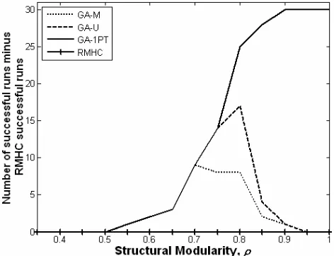
Figure 4 shows the comparative performance of each type of GA against a RMHC: the difference in number of successful runs for each value of . The number of successes out of 30 runs for each
[image:6.595.314.540.268.402.2]algorithm is also tabulated in Table 1; a run is considered successful if it found at least one of the two global optima. No graphs displaying progression of individual runs are displayed here for reasons of space, but two items merit reporting. For all GA methods on the = 1 problem, both solutions to each block are discovered in at least one member of the population rapidly, within 126,500 ± 17,336 generations for GA-1PT. The diversity maintenance provided by DC is sufficient to preserve candidates with these module solutions throughout experiments once they have been discovered – whether these are correctly recombined to produce globally optimal solutions depends on the algorithm, as shown in Table 1. The mean time to hit one of the global solutions for GA-1PT is 1,201,000 ± 137,816 evaluations.
Table 1: Success rates out of 30 repeats for each algorithm, across a range of values for structural modularity,
GA-1PT GA-U GA-M RMHC
1.00 30 0 0 0
0.95 30 0 0 0
0.90 30 1 1 0
0.85 30 6 4 2
0.80 30 22 13 5
0.75 30 30 24 16
0.70 30 30 30 21
0.65 30 30 30 27
0.60 30 30 30 28
0.55 30 30 30 29
0.50 30 30 30 30 For = 0, there is no discrimination between any of the algorithms tested, which is unsurprising given that no non-global local optima exist. Inability to discriminate continues up to = 0.5. As increases above this value, the hill climber becomes insufficient to solve the problem, but the population-based methods all succeed, even if they do not use crossover correctly; thus the distinction between the RMHC and all of the GA methods increases. As rises above 0.8 we note that the discrimination between the mutation-only GA and uniform crossover GA versus the RMHC decreases as these methods are no longer sufficient to deal with all of the local optima present; the only method which is significantly distinct from the RMHC is the one-point crossover GA. This is because one-point crossover can correctly swap in well-adapted blocks from other individuals. At the fully modular end of the scale, the discrimination between the hill climber and GA-1PT is maximal. Whilst both GA-U and GA-M outperformed the RMHC for some partially structured problems, neither are sufficient to solve the cleanly modular problem at all. The mutation-only RMHC is distracted by the strength of the internal weights and as such is not sufficient to find a global optimum amongst the abundant local optima. The mutation-only GA-M method is effectively a population of hill climbers, and whilst poor performing, appears to be a more efficient way of dividing the evaluations than the RMHC to find the right optima. As mentioned, a number of mutation rates were tried, and although the results are only shown for the best found, it is worth noting why we would not expect any alternative rate to be successful. When = 1, on the order of k=
N bits need to be
changed correctly in order to escape a local optimum. It should be obvious that low mutation rates are not sufficient, as simply not enough loci will be changed. On the other hand, we could
Figure 4. Discrimination of GA strategies when compared with a RMHC. The discrimination is strongest between GA-1PT
[image:6.595.49.285.507.688.2]select a mutation rate that is high enough to give k bit changes on average. But these k changes must occur at exactly the right loci and not disrupt any other loci, which is also infeasible when k is large.
The GA using uniform crossover can solve some of the messier problems. It slightly outperforms GA-M because it focuses variation appropriately [24]. However as approaches 1 preserving linkage becomes essential and this crossover method cannot maintain and recombine the 20 bit blocks, and the global optima are not found at all for the cleanly modular problem. The second method using crossover, GA-1PT, is successful across the full range of structural modularity. This is because it can exploit the modularity by composing candidate solutions from different combinations of module solutions, and is guided by the external dependencies in order to select for the correct combinations. Note that it is important that the population has sufficient time to find good solutions to blocks (such that external dependencies become more noticeable and can guide selection on blocks appropriately) before the population is allowed to converge to a particular solution at any block partition. Higher crossover rates seem to promote premature converge to block configurations before external dependencies are optimised, but further experimentation is needed to understand this fully. One alternative is the use of a subdivided population with more usual crossover rates [34].
4.
DISCUSSION
The results in the previous section show that ‘tuning in’ the structural modularity in the VSMP adjusts how discriminatory the problem is when comparing crossover and mutation. An algorithm using only mutation can solve non modular instances, but as the structural modularity is increased success rates are significantly impacted. However when the type of crossover that can correctly exploit this modularity is used, performance is unaffected. This supports the notion that the GA is indeed able to utilise the modular structure to solve these problems.
In order for the GA to reliably solve the VSMP at = 1, it requires two phases of search: an initial discovery of module solutions, and a second exploration of module combinations. The initial discovery is easy since monotonically increasing gradients exist to both solutions, and we see that even the mutation-only GA reliably discovers and maintains both solutions for all blocks in the problem. The second phase of exploring different module combinations requires a more sophisticated algorithm to work reliably. Specific order-k mutations are required in order to move between module-solution configurations, which are essentially unavailable via mutation for blocks of large k. However a crossover mechanism can provide such variation by recombining module solutions from different candidates, which traverses the fitness landscape in an altogether different manner.
The representation used for the VSMP permits a wide range of problems to be expressed. The specific problem used in this paper is a fairly simple problem with modular interdependency, which is sufficient to illustrate its adjustable discriminative capacity, but the representation allows much more. To start with, a number of dimensions within which the modularity can be varied are suggested in section 2.6. Using different subfunctions amongst the pairwise fitness contributions has the potential to make problems significantly more difficult as the deviance from homogeneity increases, in contrast to the decrease in difficulty
brought about by the decrease in structural modularity demonstrated here. One further way to vary the modularity present is to vary the tightness of linkage, which could be of value when investigating the robustness of linkage learning algorithms over a range of degrading linkage, for instance. In this paper only a single level of hierarchy is modelled, but the VSMP can also represent hierarchically modular problems, as is demonstrated in [32] where a version of the Hierarchical If-and-only-If is constructed with a similar approach.
5.
CONCLUSION
The results of the simulated experiments and consequent discussion support the fundamental claims of this paper, that this method of describing modular problems has the ability to vary the extent to which it discriminates the capabilities of mutation and crossover based methods. We find that when the problem has no structure the performance of all methods, crossover-based and mutation-based, are equal with respect to the percentage of runs that find a global optimum. We also find that when the modularity of the problem is strong the problem clearly discriminates between crossover-based and mutation-based methods in this respect. Specifically, the GA with deterministic crowding and one-point crossover is still able to find the globally optimal solutions in all runs, whereas other methods fail in all attempts. In between we see that the difference in performance between the GA with crossover and mutation-based methods increases monotonically as this type of modularity is increased. These results agree with simple intuitions about the utility of the GA with respect to manipulating building blocks.
6.
REFERENCES
[1] Culberson, J.C. Mutation-Crossover Isomorphisms and the construction of Discriminating Functions. Evolutionary
computation 2(3): 279-311, 1995
[2] Dauscher, P., Polani, D. and Watson, R. A. A Simple Modularity Measure for Search Spaces based on Information Theory. Proceedings of Artificial Life X, 2006
[3] Deb, K. and Goldberg, D.E. Analyzing Deception in Trap Functions. In Whitley, D. (ed) Foundations of genetic
algorithms 2, Morgan Kaufmann, CA pp 93-108, 1993
[4] de Jong, E.D., Watson, R.A. and Thierens, D. A generator for hierarchical problems. GECCO Workshop on the Theory
of Representations, 2005
[5] De Jong, K.A. An analysis of the behaviour of a class of
genetic adaptive systems. Doctoral Thesis, Department of
Computer and Communication Sciences, University of Michigan, Ann Arbor, 1975
[6] Forrest, S. Mitchell. M. What Makes a Problem Hard for a Genetic Algorithm? Some Anomalous Results and Their Explanation. Machine Learning 13: 285-319, 1993 (1993a) [7] Forrest, S. Mitchell. M. Relative Building-block fitness and
the building block hypothesis. In Whitley, D. (ed)
Foundations of genetic algorithms 2, Morgan Kaufmann, CA
pp 109-126, 1993 (1993b)
[8] Goldberg, D.E. Genetic Algorithm in Search, Optimization
and Machine Learning. Addison-Wesley, Reading, MA,
[9] Harik, G.R. Learning gene linkage to efficiently solve
problems of bounded difficulty using genetic algorithms.
PhD dissertation, department of computer science and engineering, University of Michigan, An Arbour, 1997 [10] Higgs, P.G. Overlaps between RNA secondary structures.
Physical review letters 76(4):704-707, 1996
[11] Higgs, P.G. RNA secondary structure: physical and computational aspects. Quarterly reviews of Biophysics 33(3):199-253, 2000
[12] Holland, J.H. Adaptation in Natural and Artificial Systems. University of Michigan Press, Ann Arbor MI, 1975 [13] Holland, J.H. Building blocks, cohort genetic algorithms,
and hyperplane-defined functions. Evolutionary computation 8(4):373-391, 2000
[14] Jansen, T. and Wegener, I. Real royal road functions: where crossover is provably essential. Discrete Applied
Mathematics 149(1-3):111-125, 2005
[15] Jones, T. Evolutionary Algorithms, fitness landscapes and
search. PhD Thesis, 95-05-048, University of New Mexico,
Albuquerque, 1995
[16] Kauffman, S.A. The origins of order: self-organisation and
selection in evolution. Oxford University Press, 1993
[17] Kauffman, S.A. and Johnsen, S. Coevolution to the Edge of Chaos: Coupled Fitness Landscapes, Poised States, and Coevolutionary Avalanches. In Artificial Life II, ed. C. Langton, et al, pp 325-370. Addison-Wesley, Reading, MA, 1989
[18] Lipson, H., Pollack, J.B. and Sih, N.P. On the origin of modular variation. Evolution 56(8):1549-1556, 2002 [19] Mahfoud, S. Crowding and Preselection Revisited. Parallel
problem solving from nature 2, pp 27-36, Elsevier, 1992.
[20] Mitchell M., Holland, J.H. and Forrest, S. When will a genetic algorithm outperform hill climbing? Advances in
neural information processing systems 6. Cowan, J.D.,
Tesauro, G. and Alspector, J.(eds) pp 51-58, 1993 [21] Morgan, S.R. and Higgs P.G. Barrier heights between
ground states in a model of RNA secondary structure. J
Physics A 31(14):3153-3170, 1998
[22] Pelikan, M., Sastry, K., Butz, M.V. and Goldberg, D.E. Hierarchical BOA on Random Decomposable Problems. In
procs Genetic and Evolutionary Computation Conference, Keijzer, M. et al. (eds), pp 431-432, 2006
[23] Segre, D., Ben-Eli, D. and Lancet, D. Compositional Genomes: prebiotic information transfer in mutually catalytic noncovelant assemblies. PNAS 97(8), pp4112-4117, 2000 [24] Shapiro, J. L. and Prügel-Bennett, A. Genetic algorithm
dynamics in two-well potentials with basins and barrier. In
Proceedings of Foundations of Genetic Algorithms - 4,
Belew, R. K. and Vose, M. D. (eds) pp 101-116, 1997 [25] Simon, H.A. The sciences of the artificial. MIT Press,
Cambridge MA, 1969
[26] Smith, M.J.S. Application-Specific Integrated Circuits. Addison-Wesley, Reading MA, 1997
[27] Spears, W.M. Crossover or Mutation? In Whitley, D. (ed)
Foundations of genetic algorithms 2, Morgan Kaufmann, CA
pp 221-237, 1993
[28] Vose, M.D. The Simple genetic algorithm: foundations and
theory. MIT Press, Cambridge MA, 1999
[29] Wagner, G.P. and Altenberg, L. Complex Adaptations and the Evolution of Evolvability. Evolution 50(3):967-976,1995 [30] Watson, R.A., Hornby, G. S. and Pollack, J.B. Modeling
building block interdependency. Proceedings of Parallel
problem solving from nature V, Eiben, A.E., et al. (eds), pp
97-106, 1998
[31] Watson, R.A. A simple two-module problem to exemplify building block assembly under crossover. In procs Parallel
Problem Solving from Nature VIII, Springer, pp. 161-171,
2004
[32] Watson, R. A. and Pollack, J. B. Modular Interdependency in Complex Dynamical Systems. Artificial Life 11(4):445-457, 2005
[33] Watson, R.A. Compositional Evolution. MIT Press, Cambridge MA, 2006
[34] Watson, R.A. and Jansen, T. A building block royal road where crossover is provably essential. In procs Genetic and
Evolutionary Computation Conference, 2007
[35] Yu, T. and Goldberg, D.E. Conquering hierarchical difficulty by explicit chunking: substructural chromosome
compression. In procs Genetic and Evolutionary