University of Southampton Research Repository
ePrints Soton
Copyright © and Moral Rights for this thesis are retained by the author and/or other
copyright owners. A copy can be downloaded for personal non-commercial
research or study, without prior permission or charge. This thesis cannot be
reproduced or quoted extensively from without first obtaining permission in writing
from the copyright holder/s. The content must not be changed in any way or sold
commercially in any format or medium without the formal permission of the
copyright holders.
When referring to this work, full bibliographic details including the author, title,
awarding institution and date of the thesis must be given e.g.
AUTHOR (year of submission) "Full thesis title", University of Southampton, name
of the University School or Department, PhD Thesis, pagination
Algorithms for Coalition
Formation in Multi-Agent Systems
by
Talal Rahwan
A thesis submitted in partial fulfillment for the
degree of Doctor of Philosophy
in the
Faculty of Engineering, Science and Mathematics
School of Electronics and Computer Science
UNIVERSITY OF SOUTHAMPTON
ABSTRACT
FACULTY OF ENGINEERING, SCIENCE AND MATHEMATICS SCHOOL OF ELECTRONICS AND COMPUTER SCIENCE
Doctor of Philosophy
by Talal Rahwan
Coalition formation is a fundamental form of interaction that allows the creation of co-herent groupings of distinct, autonomous, agents in order to efficiently achieve their individual or collective goals. Forming effective coalitions is a major research chal-lenge in the field of multi-agent systems. Central to this endeavour is the problem of determining which of the possible coalitions to form in order to achieve some goal. This usually requires calculating a value for every possible coalition, known as thecoalition value, which indicates how beneficial that coalition would be if it was formed. Now since the number of possible coalitions grows exponentially with the number of agents involved, then, instead of having a single agent calculate all these values, it would be more efficient to distribute this calculation among all agents, thus, exploiting all com-putational resources that are available to the system, and preventing the existence of a single point of failure.
iii
Once the coalitional values are calculated, the agents usually need to find a combination of coalitions in which every agent belongs to exactly one coalition, and by which the overall outcome of the system is maximized. This problem, which is widely known as thecoalition structure generation problem, is extremely challenging due to the number of possible combinations which grows very quickly as the number of agents increases, making it impossible to go through the entire search space, even for small numbers of agents. Given this, many algorithms have been proposed to solve this problem using different techniques, ranging from dynamic programming, to integer programming, to stochastic search, all of which suffer from major limitations relating to execution time, solution quality, and memory requirements.
Nomenclature ix
Acknowledgements xii
1 Introduction 1
1.1 Coalition Formation in Multi-Agent Systems . . . 3
1.1.1 Coalitional Value Calculation . . . 4
1.1.2 Coalition Structure Generation . . . 5
1.1.3 Payoff Distribution . . . 7
1.2 Research Objectives . . . 8
1.3 Research Contributions . . . 12
1.4 Thesis Structure . . . 16
2 Literature Review 18 2.1 Distributing the Coalitional Value Calculations . . . 18
2.2 Solving the Coalition Structure Generation Problem . . . 21
2.2.1 Low Complexity Algorithms that return an Optimal Solution . . 22
2.2.2 Fast Algorithms that provide no Guarantees on their Solutions . 27 2.2.3 Anytime Algorithms that return Solutions within a Bound from the Optimal . . . 29
2.3 Summary . . . 40
3 Distributing the Coalitional Value Calculations 42 3.1 The DCVC Algorithm . . . 42
3.1.1 The Basic Algorithm . . . 43
3.1.2 Modifying the Coalitions to which an Agent is Assigned . . . . 52
3.1.3 Considering Different Computational Speeds . . . 56
3.2 Generalizing DCVC to deal with Subsets of Agents . . . 58
3.2.1 Searching throughP . . . 59
3.2.2 Repeating the Entire Distribution Process . . . 62
3.2.3 Comparing the Distribution Efficiency . . . 63
3.3 Computational Complexity . . . 64
3.3.1 Searching throughP . . . 66
3.3.2 Repeating the Entire Distribution Process . . . 73
3.4 Performance Evaluation . . . 74
CONTENTS v
3.4.1 DistributingP . . . 77
3.4.1.1 Distribution Time . . . 77
3.4.1.2 Communications between the Agents . . . 78
3.4.1.3 Redundant Calculations Performed . . . 78
3.4.1.4 Memory Requirements . . . 79
3.4.1.5 Equality of the Agents’ Shares . . . 80
3.4.2 DistributingP∗ . . . 81
3.4.2.1 Distribution Time . . . 81
3.4.2.2 Communications Between the Agents . . . 82
3.4.2.3 Redundant Calculations Performed . . . 83
3.4.2.4 Memory Requirements . . . 83
3.4.2.5 Equality of the Agents’ Shares . . . 84
3.5 Summary . . . 85
4 Solving the Coalition Structure Generation Problem 87 4.1 Search Space Representation . . . 87
4.1.1 Partitioning the Search Space . . . 88
4.1.2 Computing Bounds for Sub-Spaces . . . 89
4.2 The Anytime Integer-Partition based Algorithm (AIPA) . . . 92
4.2.1 Step 1: Computing Bounds . . . 93
4.2.2 Step 2: Selecting and SearchingF−1[{G}] . . . . 95
4.2.2.1 SelectingF−1[{G}]. . . . 95
4.2.2.2 Searching withinF−1[{G}]. . . 97
4.3 Experimental Evaluation . . . 105
4.3.1 Experimental Setup . . . 106
4.3.2 Results . . . 106
4.4 Summary . . . 110
2.1 Shehory and Kraus’s distribution algorithm. . . 19 2.2 Example of how Shehory and Kraus’s distribution algorithm works (given
5 agents). . . 20 2.3 The DP algorithm for coalition structure generation. . . 24 2.4 Example of how the DP algorithm performs, given a set of agentsA=
{1,2,3,4}. Here, the arrows show some of the cases where a solution of a subsubproblem is used to find the solution of a subproblem . . . 25 2.5 The coalition structure graph for 4 agents. . . 30 2.6 Sandholm et al.’s algorithm for coalition structure generation. . . 31 2.7 Showing how the bound provided by Sandholm et al.’s algorithm
im-proves with the number of coalition structures examined (given 24 agents). 33 2.8 Dang and Jennings’s algorithm for coalition structure generation. . . 34 2.9 Comparison of the searching path between Dang and Jennings’s and
Sandholm et al.’s algorithms. . . 35 2.10 Showing how the bound provided by the two algorithms improves with
the number of coalition structures examined (given 24 agents). . . 36 2.11 Showing how the bound provided by different algorithms improves with
the number of coalition structures examined (given 24 agents). Here, the X values are plotted on a log-scale. . . 37 2.12 Showing the number of coalitions structures searched every time a new
bound is established (given 24 agents). Here, the X values are plotted on a log scale. . . 38
3.1 The DCVC algorithm (basic version). . . 45 3.2 SettingM to the coalition located atindexs,iinLs. . . 48 3.3 Finding a coalition atindex= 46in the listL5 of coalitions of9agents. 49 3.4 The resulting distribution for all possible coalitions of6agents. . . 52 3.5 Example for settingM to the coalition before it in the listL5 of9agents. 53 3.6 For the case of 7 agents, the figure shows how a2 and a6 set M from
one coalition to another through the listsL4,2 andL4,6 respectively. . . . 53 3.7 For the case of 31 agents with equal computational speeds, the figure
shows the time required for each agent to setM to the coalitions in its share. (A) shows the case where each agent’s share consists of a set of sequential coalitions, while (B) shows the case where each agent’s share is divided into two sub-lists. . . 54 3.8 The DCVC algorithm (final version). . . 65
LIST OF FIGURES vii
3.9 The total number of operations required for distributing P∗, and that is given 30 agents, where each agent ai searches through Pi without maintaining its share ofP∗. . . 68 3.10 Given that A¯∗removed = φ, and A¯∗added 6= φ, the figure shows the total
number of operations required to distribute P∗, and that is given 30 agents, where each agent maintains its share ofP as well asP∗. . . 71 3.11 Given that A¯∗removed 6= φ, and A¯∗added = φ, the figure shows the total
number of operations required to distribute P∗, and that is given 30 agents, where each agent maintains its share ofP as well asP∗. . . 72 3.12 The number of operations required for distributingP∗given 30 agents,
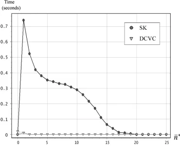
and that is using different distribution methods. . . 75 3.13 For the case of 25 agents, the figure shows the time required to distribute
P∗amongA∗, given different values ofn¯∗. . . 83 4.1 Representing the space using G and F−1[{G}] and the lists of
coali-tions Ls. The different levels represent layers used in previous rep-resentations where worst case bounds can be established by searching particular layers. The numbers represent the indices of the agents (e.g. 1 fora1, 4 fora4). . . 90 4.2 Example of how sub-spaces are pruned based on the bounds calculated.
Here, each box represents a sub-space, and the width of each box rep-resents the relative number of coalition structures within the sub-space. 94 4.3 A naive technique for cycling through the coalition structures within
F−1[{G}]. . . . 96 4.4 A naive technique for cycling through the coalition structures within
F−1[{G}]. . . . 99 4.5 Example of how the basic cyclation technique results in a number of
in-valid combinations being examined, as well as redundant combinations being generated, and that is given A = {a1, a2, a3, a4, a5, a6, a7} and
G={2,2,3}. . . 100 4.6 Example of our novel cyclation technique, givenA={a1, a2, a3, a4, a5, a6, a7}
andG={2,2,3}. . . 102 4.7 Applying branch-and-bound while searching through the coalition
3.1 The lists of possible coalitions for 6 agents. . . 44
3.2 For the case of 30 agents, the table shows the difference between the agent that had the biggest share of calculations and the one that had the smallest, given different values ofn∗. . . 66
3.3 The time required (in seconds) for the distribution process. . . 77
3.4 The total number of bytes that had to be sent between the agents. . . 78
3.5 The total number of redundant values that were calculated. . . 79
3.6 The minimum number of bytes required per agent to save the necessary coalitions. . . 80
3.7 The difference between the agent that had the biggest share of calcula-tions and the one that had the smallest. . . 81
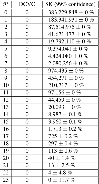
3.8 For the case of 25 agents, the total number of redundant values that were calculated, given different values ofn¯∗. . . 84
3.9 For the case of 25 agents, the table shows the difference between the agent that had the biggest share of the calculations and the one that had the smallest, given different values ofn¯∗. . . 85
Nomenclature
Chapter 2
A the set of agents
ai theithagent inA
n the number of agents inA
v(C) the coalitional value of coalitionC CS a coalition structure
Ci theithcoalition in a coalition structure
CS∗ an optimal coalition structure
C∗ a coalition inCS∗
CSq∗ the best of all the coalition structures that do not include any coalition of sizes > q CSq0 the best solution found by Shehory and Kraus’s CSG algorithm
I the size of largest coalition inCSq0
q the maximum size of coalitions considered by the SK algorithm
Siq the set of coalitions that include up toqagents includingai
Sijq the subset of the coalitions inSiq in whichaj is a member
Pi the long-term commitment list for an agentaiusing the SK algorithm
f1(C) the optimal way of splitting coalitionCinto two coalitions
f2(C) the value off1(C)
B the bound on the quality of the solution found
Li theithlevel in the coalition structure graph
SL(n, k, c) the set of all coalition strucutres whose cardinality is equal to k, and contain at least one coalition whose cardinality is not less thanc
SL(n, c) the set of all coalition structures whose cardinality is between 3 and n−1, and contain at least one of these coalition whose cardinality is not less thatc
Z ann×2nmatrix of zeros and ones
X a vector containing2nbinary variables
eT a vector ofnones
Chapter 3
S the set of permitted coalitional sizes in DCVC
Ls an ordered list of possible coalitions of sizes
Ns the number of coalitions inLs
Ci,s the coalition located at indexiin the listLs
cji,s thejthelement inC i,s
Ls,i agentai’s share ofLs
Ns,i the number of coalitions inLs,i
indexs,i the index inLsat whichLs,iends
Ljs,i thejthsub-list ofL s,i
Ns,ij the number of coalitions inLjs,i indexjs,i the index inLsat whichLjs,iends
N0 the number of additional coalitions that are not covered by the agents’ equal shares
A0 the sequence of agents in which each agent calculate one additional value
α a value maintained by the agents to determine the elements ofA0 n! nfactorial
Csn the number of all possible coalitions of sizesout ofnagents
M a space of memory that is sufficient to maintain one coalition at a time
mi theithelement inM
β the point inM after which all the values need to be updated to shiftM one step in
the list of coalitions
pascal thePascal matrix
ti the time required foraito perform a pre-determined amount of operations
V the space of vectors in which, for every vector→v∈V, we havePn
i=1vi =Ns
A∗ the set of agents that are currently able to join any coalition
n∗ the number of agents inA∗ A∗prev the previous value ofA∗ n∗prev the number of agents inA∗prev
¯
A∗ the set of agents that arecurrentlynot able to join other coalitions ¯
a∗i theithagent inA¯∗ ¯
n∗ the number of agents inA¯∗
op(¯n∗) the number of required operations givenn¯∗ ¯
A∗prev the set of agents that were not able to join other coalitions during the previous
re-calculation process
¯
NOMENCLATURE xi
¯
A∗removed the set of agents that belong toA¯∗prev, but do not belong toA¯∗
¯
n∗removed the number of agents inA¯∗removed
¯
A∗added the set of agents that belong toA¯∗, but do not belong toA¯∗prev
¯
n∗added the number of agents inA¯∗added
P the set of coalitions taken into consideration
P∗ the subset ofP in which every coalition contains only members ofA∗ Pprev∗ the previous value ofP∗
tempi a temporary list used to maintainai’s share ofP∗
Chapter 4
maxs the maximum value of the coalitions of sizes
mins the minimum value of the coalitions of sizes
avgs the average value of the coalitions of sizes
V(CS) the value of coalition structureCS
P(A) the set of possible coalition structures
F(CS) the cardinality of the coalitions ofCS G coalition structure configuration
gi theithelement inG
G(s) the multiplicity ofsinG
G the set of possible coalition structure configurations
F−1[{G}] the pre-image of a configurationG
SG the cartesian product of the coalition listsLs, wheres ∈G
CSG∗ the best coalition structure inF−1[{G}]
U BG upper bound for the values of the coalition structures contained inF−1[{G}]
U Bmax the maximum of all upper bounds of the sub-spaces inF−1[{G}], whereG∈ G
AV GG the average of the values of the coalition structures contained inF−1[{G}] G2 the set of configurations containing two elements
AV G∗G2 the maximum of all average values of the sub-spaces inF−1[{G}], whereG∈ G2
CS0 the best coalition structure obtained by scanning the input as specified in AIPA
E(G) the underlying set of elements ofG
M a space of memory that is sufficient to maintain one coalition structure at a time
Mi theithelement ofM
Ak the set of agents that are not members ofC1, . . . , Ck−1
LCi
First of all, I would like to express my sincere gratitude to my supervisor, Professor Nick Jennings, who has helped me shape my research from the very first day, and who has always been supportive and patient throughout the whole period of my study until the very last day before submission.
I would like to thank my family, starting with my wife, Shaza, who had to go through difficult times to help me fulfill my dream, and for being so kind, patient, loving, caring, cheerful, and most importantly, for being the greatest mother for my baby child, Ameer. I would like to thank my brother, Iyad, for believing in me, and for helping me apply for the scholarship that got me this far. I would also like to thank my twin brother, Tarek, who would always understand me and cheer me up whenever I felt uneasy. I would also like to thank my parents for their endless support.
I would like to express my gratitude to the people with whom I co-authored a num-ber of papers during the period of my study, namely Sarvapali Ramchurn, Viet Dung Dang, and Andrea Guovanucci. I would also like to thank all my colleagues at work for creating such an enjoyable working environment.
I am also grateful to the anonymous reviewers of AAAI-05, IJCAI-07, AAAI-07, and AIJ, for giving us much useful feedback. I would also like to thank Tuomas Sandholm, Onn Shehory, and Gal A. Kaminka for their helpful comments.
Last but not least, I would like to acknowledge the DIF-DTC project (8.6) on Agent-Based Control for funding me during the years of my study.
To my wife, Shaza, for being by my side when I needed her
the most.
Introduction
Open distributed computing applications are becoming increasingly common-place in our society. In most cases, these applications are composed of multiple actors or agents, each with its own aims and objectives. In such complex systems, dependencies between these multiple agents are inevitable, and generally speaking, they cannot all be predicted in advance.
In this context, an agent can be defined as a computer system that is situated in some environment, and that is capable of autonomous action in this environment in order to meet its design objectives [Wooldridge and Jennings, 1995]. Here, autonomy refers to the agent’s ability to act without the intervention of humans or other systems. An agent usually has a repertoire of actions by which it can influence its environment, and the key problem facing the agent is then to decide which of these actions to perform in order to meet its design objectives [Wooldridge, 2000]. An agent is considered to be intelligentif it is capable of flexible autonomous action. In this context, flexibility refers to the agent’s ability to be reactive(i.e. respond in a timely fashion to changes in the environment), proactive (i.e. exhibit goal-directed behaviour and take initiative where appropriate), andsocial(i.e. interact with other agents and, possibly, humans).1
As is currently the case in most existing research on multi-agent systems, we implicitly assume that the agents we deal with are intelligent. Therefore, throughout this thesis, we will use the term “agent” as an abbreviation for “intelligent agent”.
Given this background, a multi-agent system is a system that consists of a number of agents, situated within the same environment, carrying out their activities within that common environment. Typically, these agents need to interact with each other in order
1For more details, see Wooldridge [2002].
Chapter 1 Introduction 2
to fulfill their objectives or improve their performance. This is because of the inevitable interdependencies that exist between the agents’ environment and design objectives. Such interactions typically involve a form of cooperation, coordination, and/or negoti-ation. In fact, it is the agents’ ability to interact with one another, and compensate for each other’s deficiencies, that makes the multi-agent systems applicable to a wide vari-ety of applications, ranging from industrial (e.g. process control and air traffic control [Jennings et al., 1995; Kinny et al., 1996]), to commercial (e.g. electronic commerce and business management [Chavez and Maes, 1996; Jennings et al., 2000]), to medical (e.g. patient monitoring and health care [Hayes-Roth et al., 1989; Huang et al., 1995]), to entertainment (e.g. games and interactive theater and Cinema [Wavish and Graham, 1996; Hayes-Roth et al., 1988]). It is also used in conjunction with other technologies such as semantic web and web services [Berners-Lee et al., 2001; Huhns, 2003].
Now, within these applications, the agents could belong to a single designer, in which case they are considered to becooperative(i.e. each agent is concerned with maximiz-ing the social welfare of the entire system, even if this does not necessarily maximize its own utility). Other applications could involve a number of agents representing dif-ferent stakeholders, each with its own goals and preferences. In this case, the agents are considered to beself-interested(i.e. they act in a way that maximizes their own utility, regardless of the consequences this could have on other agents’ utilities). Note that the designer of such systems typically requires an enforcement mechanismin order to in-centivize these self-interested agents to act in a cooperative manner.2 In this thesis, we
are primarily concerned with cooperative systems, but the algorithms we develop could be applied in a self-interested environment if an appropriate enforcement mechanism was developed. However, such extensions are beyond the scope of this thesis.
Moreover, in both the cooperative and the selfish cases, the system designer needs to ensure that the agents are organized such that the roles, relationships, and authority structures which govern the agents’ behaviour are clearly defined [Horling and Lesser, 2005]. Different organizational paradigms include hierarchies, teams, federations, and many others. Each of these paradigms has its own strengths and weaknesses, making it more suitable for some problems, and less suitable for others. Among the organi-zational paradigms that are becoming increasingly important in multi-agent systems is the coalitional organization (formally defined in Section 1.1). This is because of its its natural fit to most scenarios where there may be no central authority to resolve possible
2A sub-field of game theory, known asmechanism design, deals with setting up the rules that
conflicts among the agents involved. Several applications of coalitional organizations have emerged in areas such as sensor networks, e-commerce, and distributed vehicle routing (see Section 1.1 for more details). However, many challenges lie in the way of creating coalitional organizations, and in this thesis we present solutions to some of these challenges that significantly improve upon previous attempts.
The remainder of this chapter sets the basic background for our work, and outlines the aims and contributions of this thesis. In particular, Section 1.1 introduces the area of coalition formation in multi-agent systems, and identifies the challenges that need to be overcome in order to facilitate the coalition formation process. Building upon this, Section 1.2 identifies the research aims and motivations of the work presented in this thesis, and Section 1.3 outlines our contributions to the state of the art. Finally, in Section 1.4, we give the overall structure of this thesis.
1.1
Coalition Formation in Multi-Agent Systems
Horling and Lesser [2005] specify the main characteristics that distinguish coalitions from other organizations as follows:
“Coalitions in general aregoal-directed and short-lived; they are formed with a purpose in mind and dissolve when that purpose no longer exists, or
when they cease to suit their designed purpose, or when the profitability is
lost as agents depart.”
Another defining feature of coalitional organizations is that, within each coalition, the agents coordinate their activities in order to achieve the coalition’s goal(s), but no coor-dination takes place among agents belonging to different coalitions (except if the coali-tions’ goals interact). Moreover, the organizational structure within each coalition is usually flat (although there could be a coalition leader acting as a representative for the group as a whole).
Chapter 1 Introduction 4
can work together to track targets of interest [Dang et al., 2006]. In distributed vehicle routing, coalitions of delivery companies can be formed to reduce the transportation costs by sharing deliveries [Sandholm and Lesser, 1997]. Coalition formation can also be used for information gathering, where several information servers form coalitions to answer queries [Klusch and Shehory, 1996].
In all of these cases, however, the coalition formation process can generally be con-sidered to include three main activities:
1. Coalitional Value Calculation – compute the value of every possible coalition that can be formed.
2. Coalition Structure Generation – compute the set of disjoint coalitions that have the maximum total value.
3. Payoff Distribution – determine the rewards that each agent in a coalition should obtain as a result of the actions taken by the coalition as a whole.
We deal with each of these activities in the following subsections.
1.1.1
Coalitional Value Calculation
One of the main challenges here, however, lies in the number of values to be calculated, which is exponential in the number of agents. One way to combat this computational explosion is to distribute this calculation among the agents, rather than having it done centrally by one agent (as is the case in most extant work). In this way, the calculation process can be done faster, and the agents can share the burden of the computations. In order to do so, however, we need an algorithm that specifies exactly how these cal-culations are to be carried out in an efficiently distributed manner. To date, the only algorithm in the literature designed specifically for this purpose suffers from major lim-itations that make it inapplicable, particularly given large numbers of agents. These include a considerable number of computations being redundantly carried out, a large number of messages being sent among the agents, and infeasibly large memory require-ments (see Section 2.1 for more details). This motivates the development of an efficient distribution algorithm that avoids all of these limitations.
1.1.2
Coalition Structure Generation
Another challenging problem that arises in the coalition formation process is that of coalition structure generation (CSG). That is, given the coalitional values, how to parti-tion the set of agents into exhaustive and disjoint coaliparti-tions. Such a partiparti-tion is called a coalition structure. For example, given a set of agentsA={a1, a2, a3}, there exist five possible coalition structures: {{a1},{a2},{a3}}, {{a1},{a2, a3}}, {{a2},{a1, a3}},
{{a3},{a1, a2}},{{a1, a2, a3}}.
To this end, it is usually assumed that every coalition performs equally well, given any coalition structure containing it (i.e. the value of a coalition does not depend on the actions of nonmembers). Such settings are known ascharacteristic function games (CFGs), where the value of a coalition is given by acharacteristic function.3 Of course,
not all settings are CFGs; in some cases, the value of a coalition might well depend on nonmembers’ actions due to positive and negative externalities:
“Negative externalities between a coalition and nonmembers are often caused
by shared resources. Once nonmembers are using a portion of the resource,
not enough of that resource is available to agents in the coalition to carry
out the planned solution at the minimum cost. Negative externalities can
3Note that knowing that the values are given by some characteristic function does not necessarily
Chapter 1 Introduction 6
also be caused by conflicting goals. In satisfying their own goals,
nonmem-bers may actually move the world further from the coalition’s goal state(s)
[Rosenschein and Zlotkin, 1994]. Positive externalities are often caused
by partially overlapping goals. In satisfying their goals, nonmembers may
actually move the world closer to the coalition’s goal state(s). From there
the coalition can reach its goals at less expense than it could have without
the actions of nonmembers”[Sandholm et al., 1999]
The more general case, in which coalition values depend on the actions of non-members, is known asnormal form games(NFGs). Note that CFGs are a strict subset of NFGs. However, many (but clearly not all) real-world multi-agent problems happen to be CFGs, see, e.g. [Sandholm and Lesser, 1997]. This is because in many real-world set-tings, a coalition’s possible actions and payoff are unaffected by the actions of nonmem-bers [Sandholm et al., 1999]. Moreover, most studies in economics consider games in characteristic forms as they tend to capture the most important properties of the agents’ interactions and permit an easy systematic analysis of the properties of these interac-tions [Mas-Colell et al., 1995].
Given the settings we deal with (i.e. CFGs), the coalition structure generation problem becomes a complete set partitioning problem [Rahwan et al., 2007b]. In more detail, given a collection of subsets of a ground set, and given a weight associated to each of these subsets, the set partitioning problem is to find an optimal4 way to partition the ground set. This is similar to our CSG problem since we also need to find an optimal way to partition the set of agents given a number of coalitions (i.e. subsets) and given a value associated to each of these coalitions. The complete set partitioning problem (where every possible subset is included in the input [Lin and Salkin, 1983]) is particu-larly similar to our CSG problem, since we also take into consideration every possible coalition. Based on this, any algorithm that is designed to solve one of these problems can also be applied to solve the other.
The CSG problem is also similar to another problem in combinatorial auctions, namely that ofwinner determination[Sandholm et al., 1999]. Such auctions involve a number of assets being simultaneously auctioned, and a number of bidders that are allowed to place bids on combinations of these assets (hence the term “combinatorial auction”). Once the auction is closed, the auctioneer needs to partition the set of assets, given the placed bid on (i.e. the weight of) every combination (i.e. subset) of these assets, such
4We call such a solutionan optimalsolution to the problem, as opposed tothe optimalsolution, since
that the overall sum of bids (i.e. the auctioneer’s revenue) is maximized [Carmton et al., 2007]. Now in case the bids were allowed on every possible combination of assets, then this again becomes very similar to the CSG problem.
In all of these problems, however, the space of possible solutions grows very rapidly with the number of elements involved, making it extremely challenging to find an op-timal solution. In particular, Sandholm et al. [1999] proved that finding an opop-timal solution is NP-complete. To combat this complexity, a number of algorithms have been developed in the past few years, using different search techniques (e.g. dynamic pro-gramming, integer propro-gramming, and stochastic search). These algorithms, however, suffer from major limitations that make them either inefficient or inapplicable, partic-ularly given large numbers of agents (see Section 2.2 for more details). Against this background, we need an algorithm that can efficiently search the space of possible so-lutions. Here, by efficient, we mean satisfying a number of properties that are specified in the following section.
Finally, note that an optimal solution to the CSG problem is one that maximizes the so-cial welfare. Moreover, unlike cooperative environments, where the agents are mainly concerned with maximizing the social welfare, the agents in a selfish environment are only concerned with maximizing their own utility. This, however, does not mean that a CSG algorithm cannot be applied in selfish multi-agent systems. This is because the designer of such systems is usually concerned with raising the overall efficiency of the system, and in many cases, this corresponds to maximizing the social welfare. Thus, by knowing the optimal coalition structure, the designer can incentivize the selfish agents to form that structure. Moreover, knowing the value of the optimal coalition structure, or knowing a value that is within a bound from that optimal, allows the designer to eval-uate the relative effectiveness of the coalition structure currently formed in the system.
1.1.3
Payoff Distribution
Chapter 1 Introduction 8
their goals. The analysis of such incentives has long been studied within the realm of
cooperative game theory. In this context, many solutions have been proposed based on different stability concepts. These include theCore, theShapley value, and the Kernel (for more details, see [Osborne and Rubinstein, 1994]). Moreover, transfer schemes have been developed to transfer non-stable payoff distributions to stable ones while keeping the coalition structure unchanged (Kahan and Rapoport [1984] provide a com-prehensive review on stability concepts and transfer schemes in game theory). Note, however, that in the case of cooperative environments, the agents are concerned with maximizing the system outcome, and thus are willing to join the coalition that max-imizes the social welfare, regardless of their share of the coalition value. Therefore, payoff distribution is less important, and the main concern is generating a coalition structure so as to maximize the social welfare.
Furthermore, it is important to note that game theory is more concerned with analysing the outcomes of interactions and the strategies of the agents rather than providing al-gorithms that the agents can use in order to actually form the coalitions. Moreover, game theoretic approaches typically assume that the coalition formation process is cen-tralized, and do not take into consideration the resource constraints of a computational environment (such as communication bandwidth and limited computation time). Given our focus on computational multi-agent systems, this is a serious shortcoming. More-over, much of the research on coalition formation in game theory has focused on super-additive environments, in which any combination of two groups of agents into a new group is beneficial [Zlotkin and Rosenschein, 1994; Kahan and Rapoport, 1984]. In such environments, the process of searching for the coalition that maximizes the system welfare is trivial, since this coalition will be the one in which every agent is a member (commonly known as thegrand coalition). This assumption, however, does not hold for many real-world applications, due to the intra-coalition coordination and communi-cation costs which increase with the size of the coalition [Sandholm and Lesser, 1997], and therefore, our focus in this thesis is mainly onnon-super additive environments.
1.2
Research Objectives
1. The distribution process should be decentralized.5 That is, no one decision maker
should be required to decide which agent calculates which values. This is because the existence of a central agent can slow down the performance of the system, and reduce its overall robustness. Specifically, having one agent in charge of handling the communication with, and coordinating the activities of, all other agents could result in a performance bottleneck. Moreover, a centralized system would have a single point of failure; if the centre fails then the whole system could crash. On the other hand, if control and responsibilities are sufficiently shared among different agents, the system can tolerate the failure of one or more of the agents.
2. Communication between the agents should be minimized. This is particularly important when the agents have limited communication bandwidth.
3. The coalitional values of all the desired coalitions should be computed (i.e., the distribution process must ensure that every value is calculatedat least once) and the agents should minimize the number of calculations that are redundantly car-ried out (i.e., it would be desirable if every value is calculatedexactly once).
4. In order to minimize the time taken, the computational load should be balanced among the agents. In other words, if the agents have equal processing capabili-ties, each one of them should compute an equal number of values, and if they have unequal capabilities, the faster computational agents should take on a greater bur-den of the calculations. This causes all the agents to finish their calculations at broadly the same time, rather than having some agents finish and wait for oth-ers who have not yet finished (which corresponds to having some of the system resources not being fully exploited).
5. The amount of memory that is required to execute the algorithm should be mini-mized. This is because the number of coalitions to be distributed grows exponen-tially with the number of agents involved. Therefore, any distribution algorithm that requires each agent to maintain its entire share in memory would require infeasibly large amounts of memory (e.g. maintaining a list of all the possible coalitions of 40 agents requires a total of 5120 GB of memory).
6. In most practical situations, the agents continuously form coalitions whenever new ones are necessary, and formed coalitions are dissolved whenever it is ben-eficial to do so. As a result of this continuous change, the process of calculating
5Note that just because a system is distributed does not necessarily mean that it is decentralized. A
Chapter 1 Introduction 10
the coalitional values is not a one-shot activity. For example, forming a coalition might correspond to a task being assigned to the coalition, or might correspond to a change in the set of resources that are available to the agents. In either case, the values need to be re-calculated to take these changes into consideration. Note that this re-calculation process might differ from the initial calculation process in that some of the agents might no longer be able to join subsequent coalitions. For example, in cases where the coalitions are not allowed to overlap (e.g. Shehory and Kraus [1995]), then after a coalition is formed, every agent that has joined that coalition is no longer available to join other coalitions (until that coalition is dissolved). Another example is in the case where each agent requires a certain number of resources in order to join a coalition (e.g. Shehory and Kraus [1998, 1996]). In this case, the agents that have now used all of their resources in one or more coalitions, can no longer be considered. Based on this, whenever a coalition needs to be formed, the algorithm must only take into consideration the subset of agents which is currently available and eligible.
7. It is desirable if the algorithm could distribute the calculations among any given subset of agents (i.e., it would be desirable if the algorithm makes no assumptions about the set of agents among which the calculations are to be distributed). This is because different cases require distributing the calculations among different sets of agents. For example, in case the tasks that are assigned to the coalitions were complex, and require a significant amount of computational effort from its members, then it might be more efficient to distribute the value calculations only among the agents that have not yet joined any coalition. On the other hand, if the coalition tasks were relatively simple, then it might be desirable for all the agents to take part in the value calculation process. After all, the agents are assumed to be cooperative, and are, therefore, willing to help each other, even if some of them were not able to join any of the coalitions for which the values are being cal-culated. In any case, having control over which agents carry out the calculations results in a more flexible distribution process.
The second aim of this thesis is motivated by the need to develop efficient algorithms for solving the coalition structure generation problem. Next, we outline a number of desiderata that are necessary, if such an algorithm is to be practically applicable:
2. Since the search space grows very quickly as the number of agents increases, it is extremely difficult to perform anexhaustive search (i.e. abrute-force search) where every possible candidate for the solution is examined (e.g. given 20 agents, the number of possible coalition structures becomes 51,724,158,235,372). There-fore, it is critical for the algorithm to avoid searching as much of this space as possible, and yet still be guaranteed to return an optimal solution. This can be done by identifying sub-spaces that have no potential of containing an optimal solution, and then pruning these sub-spaces before they are searched. Moreover, whenever an optimal solution is found, it is critical to have the ability to con-firm that this is indeed the optimal, and to stop the search accordingly, instead of proceeding with the search in the hope that a better solution can be found.
3. Since the agents are usually limited in their computational resources, and have limited memory space, then the CSG process should have minimal memory and computational requirements. For example, we wouldn’t want the agents to matain in memory every possible coalition structure, because this would require in-feasibly large amounts of memory (for example, maintaining in memory every possible coalition structure for 20 agents would require 538,600 GB)
4. It is desirable for the algorithm to beanytime. That is, it would be desirable if the algorithm can quickly return an initial solution, and then improve the quality of its solution as it searches more and more of the space, until it finds an optimal one. This is particularly important since the search space grows exponentially with the number of agents involved, meaning that the agents might not always have suf-ficient time to run the algorithm to completion. Moreover, being anytime makes the algorithm more robust against failure; if the execution is stopped before the algorithm would have normally terminated, then it would still provide the agents with a solution that is better than the initial solution, or any other intermediate one.
Chapter 1 Introduction 12
than, say,98% of the optimal solution, and if there are still millions of coalition structures that still need to be searched, then one could decide to stop the search simply because this small improvement is not worth the effort. Of course, for this to happen, we would need the bound to be as small as possible6 (for example,
if the algorithm was only able to guarantee that the solution quality is not worse than, say,1%of the optimal solution, then the agents would most likely carry on with the search, because the guarantee is simply not good enough).
With the current state-of-the-art algorithms, we consider the formation of optimal coali-tion structures to be theoretically applicable, but practically infeasible, particularly given large numbers of agents. Therefore, by developing algorithms that meet the design objectives specified earlier, we aim at making coalition formation techniques applicable to a wider range of practical situations and real-world scenarios.
1.3
Research Contributions
Against the research aims outlined above, this thesis makes significant contributions to the state of the art in two of the main stages of the coalition formation process, namely, the coalitional value calculation stage, and the coalition structure generation stage. First, we shall outline the contributions made to the coalitional value calculation stage:
1. We developed a novel algorithm, called DCVC, for Distributing the Coalitional Value Calculations among cooperative agents [Rahwan and Jennings, 2005, 2007]. In more detail, DCVC ensures that each agent is assigned some part of the cal-culations such that the agents’ shares are exhaustive and disjoint.7 Moreover, the algorithm is decentralized, requires no communication between the agents, and distributes the calculations equally among the agents.8 The algorithm also en-ables each agent to perform its share of calculations without having to maintain in memory more than one coalition. Finally, the algorithm makes no assump-tions about the agents that need to take part in the calculation process (i.e. it can distribute the calculation among any given set of agents).
6Here, the smaller the bound, the better it is, and the smallest possible bound is 1, which corresponds
to the solution being an optimal one.
7In other words, the agents’ shares are guaranteed to cover the entire set of values to be calculated,
and every value is guaranteed to be calculated by no more than one agent.
8In case the total number of coalitions was not be divisible by the number of agents, the size of the
2. We discuss why, in order to let the agents finish their calculations at the same time, it is not sufficient to considerhow manycoalitions an agent is assigned, but alsowhichcoalitions an agent is assigned. We also show how this can improve the performance of our algorithm.
3. We show how DCVC can be modified to reflect the variations in the agents’ com-putational speeds, and prove that the resulting distribution minimizes the compu-tation time.
4. We analyse the different cases in which only a subset of agents is available or eligible to join a coalition, and discuss a number of methods for distributing this subset. We then calculate the exact number of operations required by each of these methods, and show that the one adopted by DCVC requires significantly fewer operations, compared to the other methods.
5. We analyse the different cases in which only a subset of agents is available or eligible to join new coalitions. We also discuss a number of methods for han-dling the distribution process in such cases. Moreover, we provide equations for calculating the exact number of operations required by each of these methods, and show that the one adopted by DCVC requires significantly fewer operations compared to the other methods.
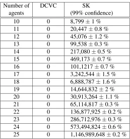
6. To benchmark the effectiveness of our algorithm, we compare it with the only other algorithm available in the literature [Shehory and Kraus, 1998]. In so doing, we show that for the case of 25 agents, the distribution process of our algorithm took less than0.02% of the time, the values were calculated using0.000006% of the memory, the calculation redundancy was reduced from 383229848 to 0, and the total number of bytes sent between the agents dropped from1146989648to0. Note that for larger numbers of agents, these improvements become exponentially better.
Having outlined our contributions to the coalitional value calculation stage, we now highlight the following specific contributions to the coalition structure generation stage:
Chapter 1 Introduction 14
of coalitionsthey contain, our representation categorizes the coalition structures into sub-spaces based on thesize of the coalitions they contain. One advantage of this representation is that, immediately after scanning the input, the agents can compute the average value of the coalition structures within each sub-space. Moreover, by scanning the input, the agents can also compute an upper and a lower bound on the best value within each sub-space. This allows the agents to immediately prune some of the sub-spaces without searching any of them, and that is simply by comparing their bounds. Another advantage of this representa-tion is that it allows the agents to analyse the trade-off between the size of (i.e. the number of coalition structures within) a sub-space and the improvement it may bring to the actual solution by virtue of its bounds. Hence, rather than constrain-ing the solution to fixed sizes, as per Shehory and Kraus [1998], agents usconstrain-ing our representation can make a more informed decision about the sizes of coalitions to choose (since each of the sub-spaces are defined by the sizes of coalitions within the coalition structures).
2. We develop a novel Anytime Integer-Partition based Algorithm (AIPA) for coali-tions structure generation which uses the representation discussed above [Rahwan et al., 2007a,b]. Specifically, AIPA returns solutions anytime, and provides very high worst-case guarantees on the quality of its solutions very quickly (almost immediately after scanning the input, the solution quality is usually guaranteed to be above90%of the optimal). Moreover, AIPA is guaranteed to return an optimal solution when run to completion, and the optimal solution is usually found after searching extremely small portions of the search space (e.g. 0.0000019% of the space for 21 agents). This is because most of the sub-spaces are usually pruned before they are searched, and whenever a sub-space is searched, the algorithm applies branch-and-bound techniques, thus, ensuring that only a few of the coali-tion structures within the sub-space are examined. In addicoali-tion, AIPA has minimal memory requirements, compared to other CSG algorithms.
to around 2 months for the best previous solution). Note that these improvements become significantly better as the number of agents increases.
4. When evaluating the quality of the bounds that AIPA provides, we compare them with those provided by other state-of-the-art anytime CSG algorithms [Sandholm et al., 1999; Dang and Jennings, 2004]. In so doing, we show that AIPA provides significantly better bounds. In more detail, we empirically show that, given 21 agents, the quality of its initial solution is usually guaranteed to be at least 92% of the optimal, as opposed to 9.52% for both Sandholm et al.’s algorithm and Dang and Jennings’s algorithm. Moreover, after searching through 0.000002% of the search space, the guarantees provided by AIPA reach100%, as opposed to 14.28%for both Sandholm et al.’s and Dang and Jennings’s algorithm.
Next, we outline the main papers that have been published in support of these contribu-tions:
1. T. Rahwan and N. R. Jennings. (2005) Distributing coalitional value calculations among cooperating agents. In Proceedings of the 25th national conference on artificial intelligence (AAAI-05)in Pittsburgh, USA. Pages 152-157.
2. T. Rahwan and N. R. Jennings. (2007) An algorithm for distributing coalitional value calculations among cooperating agents.Artificial Intelligence (AIJ). 171(8-9). Pages 535-567.
3. T. Rahwan, S. D. Ramchurn, V. D. Dang and N. R. Jennings. (2007) Near-optimal anytime coalition structure generation. InProceedings of the 20th International Joint Conference on Artificial Intelligence (IJCAI-07)in Hyderabad, India. Pages 2365-2371.
4. T. Rahwan, S. D. Ramchurn, A. Giovannucci, V. D. Dang and N. R. Jennings. (2007) Anytime optimal coalition structure generation. In Proceedings of the 22nd conference on artificial intelligence (AAAI-07)in Vancouver, Canada. Pages 1184-1190.
Chapter 1 Introduction 16
1.4
Thesis Structure
In the remainder of this thesis, we describe the algorithms available in the literature, and then present our algorithm for distributing the coalitional value calculations among cooperative agents, as well as our algorithm for solving the coalition structure genera-tion problem. This is achieved through the course of the remaining chapters, which are structured as follows:
• In chapter 2, we describe, in detail, the algorithms that are currently available
in the literature for distributing the coalitional value calculation, as well as those available for solving the coalition structure generation problem. We also discuss their limitations against the requirements that we placed earlier in this chapter, thus, motivating the work that we present later in the proceeding chapters.
• In chapter 3, we start by presenting a basic version of our algorithm for distribut-ing the coalitional value calculations (DCVC), where the agents are assumed to be homogeneous, and every agent is assumed to be able to join new coalition(s). We later show how the algorithm can be modified to reflect variations in the agents’ computational capabilities so that the distribution is optimal, and show how the algorithm can be generalized to the case where some agents might no longer be able/allowed to join new coalitions. We also discuss different approaches to the value re-recalculation process, analyse their computational complexity, and show that our approach significantly outperforms other approaches. Finally, we bench-mark our algorithm against the only other algorithm available in the literature for this purpose, and explain the reasons that make our algorithm significantly better in terms of execution time, communication and memory requirements, distribu-tion quality, and number of redundant calculadistribu-tions performed.
quality of the worst-case guarantees provided by our algorithm, we compare it with the state of the art algorithms designed for this purpose, and show that our guarantees are significantly better.
Chapter 2
Literature Review
In this chapter, we discuss the existing literature and highlight the limitations of each of the available algorithms, thus, motivating the research objectives of this thesis. In more detail, Section 2.l discusses the only algorithm in the literature that is designed specifically for distributing the coalitional value calculations among cooperative agents, while Section 2.2 identifies the different approaches to the coalition structure generation problem. Section 2.3 summarizes this work.
2.1
Distributing the Coalitional Value Calculations
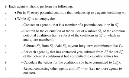
As mentioned earlier, there has been no work reported in the multi-agent systems litera-ture, either centralized or decentralized, on this problem apart from that due to Shehory and Kraus [1998] (henceforth called SK).1A slightly modified version of this algorithm also appears in [Shehory and Kraus, 1995, 1996]. The algorithm works by making the agents negotiate about which of them performs which of the calculations. In particular, Figure 2.1 details exactly how the algorithm works. Note that the figure only shows the steps that are required for each agent to know its share of calculations (i.e. the figure does not show the steps that are performed to calculate the coalitional values them-selves), and that is because we are only interested in the distribution process. Also note that Shehory and Kraus assume that the coalitions are only allowed to contain up toq
agents. This is desirable since there could be cases where only coalitions of particular sizes need to be taken into consideration (e.g. if it was known in advance that each of the tasks to be performed requires at least 3 agents, and at most 5 agents, then there
1In addition to this distribution algorithm, Shehory and Kraus [1998] present an algorithm for
coali-tion structure generacoali-tion. This algorithm, however, is discussed later in Seccoali-tion 2.2.
would be no need to consider any of the possible coalitions of sizes{1,2,6,7, . . . , n}). Figure 2.2 shows an example of how the algorithm works given 5 agents.
1: Each agentai should perform the following:
2: •Put inSiqevery potential coalition that includes up toqagents includingai.
3: •WhileSiqis not empty do:
4: – Contact an agentaj that is a member of a potential coalition inSiq.
5: – Commit to the calculation of the values of a subsetSijq of the common potential coalitions (i.e. a subset of the coalitions inSiqin whichai andaj are members).
6: – SubtractSijq fromSiq. AddSijq to your long-term commitment listPi.
7: – For each agentak that has contacted you, subtract fromSiqthe setS q ki of the potential coalitions it had committed to calculate values for.
8: – Calculate the values for the coalitions you have committed to(Sijq).
9: – Repeat contacting other agents untilSiq =ai (i.e., no more agents to contact).
FIGURE2.1: Shehory and Kraus’s distribution algorithm.
The main advantage of this algorithm is that it operates in a decentralized manner. How-ever, the algorithm suffers from the following major limitations:
• The algorithm requires many messages to be sent between the agents, most of which are exponentially large. This is because each agent ai contacts the same agents several times,2and every time an agent (ai) contacts another (aj), it has to send an exponentially large list of coalitions, which is Sijq (see step 7 in Figure 2.1).
• Although the algorithm guarantees that every value is calculated at least once, it does not guarantee that each value is calculated exactly once. In fact, when calculating the number of values that were redundantly carried out, we found that this number was exponentially large (see Section 3.4 for more details). This is mainly because the agents have very limited information about each others’ commitments. For example, given 5 agents: a1, a2, a3, a4, a5, then ifa1 contacts
2The reason behind this is that whena
icontactsaj, it commits toa subsetof the coalitions inSiqthat
containaj, meaning thataimight later contactaj again, and commit to another subset of the common
[image:34.596.105.532.142.402.2]Chapter 2 Literature Review 20
a2 and commits to calculate the values of some common coalitions, including
{a1, a2, a3, a4}, and at the same time,a3 contactsa4and commits to calculate the values of some common coalitions, including {a1, a2, a3, a4}, then the value of
{a1, a2, a3, a4}would have been calculated twice.
• The memory requirements grow exponentially with the number of agents in-volved. This is because each agent ai needs to maintain the set of potential coalitions in which it is a member, which is Siq (see step 2 in Figure 2.1), as well as the lists that are being received from other agents. Note that each agent might receive several lists simultaneously (a worst-case scenario involves receiv-ing messages from every other agent in the system), in which case the agent needs to have sufficient memory space to maintain all of these lists.
• The algorithm provides no guarantees on the quality of its distribution. Specifi-cally, given homogeneous agents, the algorithm does not guarantee that the agents’ shares are equal, and given heterogeneous agents (i.e. with different computa-tional speeds), the algorithm does not guarantee that these differences are effi-ciently reflected in the distribution.
These limitations make the algorithm both inefficient and inapplicable for large numbers of agents. Against this background, Chapter 3 presents a distribution algorithm that avoids all of these limitations, and meets all of the design objectives that were specified earlier in Section 1.2 (a comparison between this and the SK algorithm can be seen in Section 3.4).
2.2
Solving the Coalition Structure Generation
Prob-lem
In this section, we provide a classification of the different algorithms that exist for solv-ing the coalition structure generation problem. Specifically, we identify the followsolv-ing classes:
• Low complexity algorithms that return an optimal solution.
• Fast algorithms that provide no guarantees on their solutions.
Chapter 2 Literature Review 22
In the remainder of this section, we discuss both the advantages and the limitations for each of these classes, and provide examples from the existing literature.
2.2.1
Low Complexity Algorithms that return an Optimal Solution
This class of algorithms is designed to return an optimal solution while minimizing the computational complexity. Note that the emphasis, here, is on providing a guarantee on the performance of the algorithm in worst-case scenarios. One might intuitively think of this class as being the most preferable of all classes. After all, what we are usually interested in is to find an optimal solution and minimize the computational complex-ity, which is exactly what defines this class of algorithms. However, if such algorithms are to be feasibly applicable, then there is an additional requirement that could even be more crucial than the aforementioned ones, and that is to return a solutionas quickly as possible. This is mainly because we are dealing, here, with an exponentially growing search space, meaning that the algorithm, given large numbers of agents, might require a significant amount of time before returning a solution. Based on this, the agents might prefer to use an algorithm that returns a“good”solution very quickly, instead of using an algorithm for which the agents have no time to run to completion. In other words, the agents might be willing to make a trade-off between the quality of the solution, and the time required to run the algorithm.
Having identified this class, we shall discuss the state of the art algorithms that belong to it. Note that the time required to run these algorithms depends solely on the number of agents involved (i.e. given the same number of agents, and given different coalition values, the algorithm performs exactly the same number of operations, regardless of the differences in the values). Before going into the details of how these algorithms work, we shall first explain the basic method upon which these algorithms are built, namely dynamic programming, and identify the problems that can generally be solved using this method.
Dynamic programming is a method for solving problems that exhibit the properties ofoptimal substructureandoverlapping subproblems[Cormen et al., 2001]:
• Overlapping subproblems means that the subproblems are not independent, that is, subproblems share subsubproblems.
A dynamic programming algorithm solves every subsubproblem just once and saves its answer in a table, thereby avoiding the work of recomputing the answer every time the subsubproblem is encountered [Cormen et al., 2001]. In our case, the optimization problem is to find the optimal partition of the set of agentsA, and the subproblem is to find the optimal partition of a subset ofA.
In this context, Yeh [1986] developed a dynamic programming algorithm for solving the complete set partitioning problem. A very similar algorithm was later developed by Rothkopf et al. [1995] for solving the winner determination problem in combinatorial auctions. Note that both algorithms can directly be applied to find optimal coalition structures, since the problems they were originally designed to solve are very similar to the CSG problem (see Section 1.1). Also note that both algorithms are very similar in that they use the same techniques, and have the same complexity. Moreover, explaining how one of them works is sufficient to understand how the other one works. Therefore, we shall only discuss one of these algorithms, namely the one developed by Rothkopf et al. (henceforth called DP). We chose this one because it is relatively simpler and easier to implement).
The algorithm is detailed in Figure 2.3, and the way it operates is based on the fol-lowing observation:
.
Observation 1.1. Let CS∗ be an optimal coalition structure and letC∗ ∈ CS∗. Also, letC∗ ⊇C1∪C2∪. . .∪Ck such that these coalitions are pairwise disjoint (i.e.Ci∩Cj =φfor all1≤i < j ≤k). Then,v(C∗)≥
Pk
i=1v(Ci).
In other words, if a coalitionC∗ belongs to the optimal coalition structure CS∗, then dividing C∗ into smaller coalitions can never result in a better value for CS∗. For example, if an optimal partition of the set A = {1,2,3,4,5,6,7,8,9}was as follows:
{{1,2},{3,4,5},{6},{7,8,9}}, then the optimal partition of the set{1,2,3,4,5}must be{{1,2},{3,4,5}}, and similarly, the optimal partition of the set{6,7,8,9}must be
{{6},{7,8,9}}. This can be proved by contradiction. Suppose that this was not the case, and that another partition of{6,7,8,9}, say{{6,7},{8,9}}, had a greater value. In this case, {{1,2},{3,4,5},{6},{7,8,9}} can no longer be an optimal partition of
A, because we could replace {6},{7,8,9} with {6,7},{8,9} and get a greater value
Chapter 2 Literature Review 24
Input:v(C)for allC ⊆A. If nov(C)is specified thenv(C) = 0.
Output:the optimal coalition structure,CS∗.
1. For alli∈ {1, . . . , n}, setf1({ai}) :={ai}, f2(ai) :=v({ai})
2. Fori:= 2 ton, do:
For allC ⊆Asuch that|C|=i, do:
(a)f2(C) :=max{f2(C\C0) +f2(C0) :C0 ⊆Cand1≤ |C0| ≤1/2|C|}
(b) Iff2(C)≥v(C), setf1(C) :=C∗ whereC∗maximizes the right hand side of (a) (c) Iff2(C)< v(C), then setf1(C) :=C, andf2(C) :=v(C).
3. SetCS∗ :={A}.
4. For everyC ∈CS∗, do: Iff1(C)6=C, then:
(a) SetCS∗ := (CS∗\{C})∪ {f1(C), S\f1(C)}. (b) Goto 4 and start with newCS∗.
FIGURE2.3: The DP algorithm for coalition structure generation.
The algorithm requires maintaining two tables in memory, namelyf1 andf2, each hav-ing an entry for every possible coalition. Specifically, given a coalitionC ⊆ A, f1(C) would be the optimal partition of C, and f2(C) would be the value of that partition.3 Note thatf1 andf2are initially not known, and the algorithm gradually computes them as it scans the input, starting from the coalitions of size 2, then 3, then 4, and so on.
To better understand how the algorithm works, let us consider the following example, whereA = {1,2,3,4}(see Figure 2.4). At first, the algorithm goes through the coali-tions of size 2, and for each of these, determines whether to split the coalition in two, or keep it as it is. For example, givenC ={1,2}, the algorithm determines whether{1,2}
is more beneficial than {{1},{2}}, and that is by comparing the values: v({1,2})and
v({1}) +v({2}). Both the solution and its value are kept inf1(C)and f2(C) respec-tively.4 The algorithm then moves to the coalitions of size 3. Here, the algorithm also determines whether to split each of these in two, but the decision is now made based onf2 rather thanv. For example, given the coalition{1,2,3}, the algorithm compares its value with the following values: f2({1}) +f2({2,3}), f2({2}) +f2({1,3}), and
f2({3}) +f2({1,2}). Similarly, the algorithm determines whether to split the coalition of size 4 in two.
3A partition of a coalitionCcan be defined as a set of coalitions{C
1, . . . , Ck}such that∪ki=1Ci =C,
and for all1≤i < j≤k, we haveCi∩Cj=φ.
4Actually, in case it was more beneficial to split the coalition in two, rather than keep it as it is, then
only one half of the solution needs to be kept inf1. This is because, by knowing one half, the other half
FIGURE 2.4: Example of how the DP algorithm performs, given a set of agents
A = {1,2,3,4}. Here, the arrows show some of the cases where a solution of a subsubproblem is used to find the solution of a subproblem
Note that, by considering all the possible ways of splitting a coalitionCin two, and by usingf2instead ofv, the optimal partition ofCcan be found. This comes from Observa-tion 1.1, which implies that ifCS∗was an optimal partition ofA, then by splittingCS∗
into two disjoint sets of coalitions, namely CS1∗ = {C1,1, . . . , C1,k1} : ∪ki=11 Ci = A1, andCS2∗ ={C2,1, . . . , C2,k2}:∪ki=12 Ci =A2, thenCS1∗ must be an optimal partition of
A1, andCS2∗ must be an optimal partition ofA2. In other words, any optimal partitions (containing more than one coalition) must consist of two optimal partitions of two sub-problems.
The last stage (step 4 in Figure 2.3) would be to find the optimal coalition structure ofA, given that we have finished computingf1 andf2for every possible coalition. This is done as follows. Suppose that the best way to splitAin two was the following: (A1,
A2),5this means that the optimal partition ofAcan be found by combining the optimal partition ofA1 with the optimal partition ofA2. Now, each of these two partitions can be found in a similar way. For example, suppose that the best way to divideA1 in two was as follows: (A1,1, A1,2), this means that the optimal partition ofA1 can be found by combining the optimal partition of A1,1 with the optimal partition of A1,2, and so on. This process is repeated until we find a coalition structure in which f1 for every
5We would know this by looking atf
1(A1))which, in this case, must contain one half of the solution
Chapter 2 Literature Review 26
coalition contains the coalition itself. In other words, every coalition is better left as it is, rather than split in two.
The saving, at this stage, comes from the fact that solutions of subproblems do not need to be recomputed over and over again. For example, we do not need to evalu-ate both{{1},{2,4}}and{{1},{2},{4}}, because we already performed the compar-ison between {2,4} and {2},{4} when calculating the best partition of{2,4}. Simi-larly, we do not need to evaluate{{2},{1,3,4}},{{2},{1},{3,4}},{{2},{3},{1,4}},
{{2},{4},{1,3}},{{2},{1},{3},{4}}, because we have already done the comparison between all the underlined parts before. The arrows in Figure 2.4 show some of the cases where the solution of a subsubproblem is used to find the solution of a subprob-lem.
The biggest advantage of this algorithm is that it runs in O(3n)time [Rothkopf et al., 1995]. This is significantly less than exhaustive enumeration of all coalition structures (which isO(nn)). In more detail, this makes the algorithm polynomial in the size of the input. The reason for this is that the input includes2nvalues, and the algorithm runs in:
O(3n) = O(2(log23)n) = O((2n)log23) (2.1)
time. Thus the complexity is O(ylog23), where y is the number of values in the input. Note that no other algorithm in the literature is guaranteed to find the optimal coalition structure in polynomial time (in the size of the input).
On the other hand, one of the biggest limitations on using this algorithm is that it cannot generate solutions anytime. This is clearly undesirable, especially given large numbers of agents, because the time required to return the optimal solution might be longer than the time available to the agents. Another limitation on this algorithm (and on dynamic programming in general) is the large number of partial solutions that must be kept in memory. Specifically, the algorithm requires maintaining3×2nvalues in memory. This is because for every coalitionC, the algorithm requires maintainingv(C), f1(C), and