Is the promotion of organic farming the most cost efficient way of achieving environmental goals? A Danish Case story

,VWKHSURPRWLRQRIRUJDQLFIDUPLQJWKHPRVWFRVWHIILFLHQW

ZD\RIDFKLHYLQJHQYLURQPHQWDOJRDOV"

$'DQLVK&DVHVWRU\ (DRAFT) /DUV%R-DFREVHQ

Danish Research Institute of Food Economics Agricultural Policy Research Division

$EVWUDFW

This paper explores the development of an agricultural specific input-output table that explicitly includes organic farming. The table is used in an Applied General Equilibrium (AGE) model of the Danish economy to analyse four different scenarios for the development of organic agriculture and their effects on selected environmental indicators. One advantage of AGE models is that they explicitly allow for substitution between inputs in production. Introducing a tax on environmentally harmful inputs, for example, will initially increase the cost of production, although the producers to a certain extent can limit the burden of such taxes by substituting away from the taxed inputs into other inputs. The extent of substitution is determined by the exogenously given elasticity of substitution.

The objective of this paper is to analyse the cost efficient ways of achieving given environmental goals and these instruments interaction with the possible role of organic farming in such environmental strategies. The first scenario explores the impacts of a consumer demand induced increase in organic farming (a market driven scenario) followed by three different policy scenarios in absence of this assumed consumer preference change.

In the first two of the policy scenarios a subsidy to agricultural land in the organic sectors is introduced to promote a movement of land into organic production with a positive environmental effect being achieved. The first of these two subsidy experiments is designed to achieve the same hectares of land being employed by organic producers as achieved in the consumer preference scenario. This does not, however, lead to the same reduction in the use of environmental harmful inputs. Therefore, in the second of these two subsidy experiments, the subsidy to organic land is determined so as to achieve the same effects on the environmental indicators. Finally, the last policy experiment introduces environmental taxes on fertilizers and pesticides generally to achieve the same effects on the environmental indicators as in the consumer preference scenario.

,QWURGXFWLRQ

Concerns about the impact of modern agriculture on the environment have in the past few decades resulted in strict legislation concerning the leaching of nitrogen from Danish farms and their use of pesticides. An often-heard argument in recent years is that conversion to organic farming is a solution to many environmental problems. Hence, in the late 1990s several initiatives to support the development of organic farming have been taken.

Until the mid-1990s organic farmland in Denmark was held at a stable level of around 1 percent of the total cultivated area. Particularly around 1994/95 increased demand for organic products and favourable support for organic production led to a significant growth in organic farmland. Today organic farmland accounts for 5 percent of the total agricultural area, and 6.6 percent if land under conversion is included. Organic milk is the most important product accounting for around 80 percent of the total value of production. The rapid increase in organic production has, however, not been followed by a similar increase in demand. After a significant preference shift towards organic products in the mid-1990s consumer tastes have only changed slowly in the most recent years. This has resulted in a situation where approximately 60 percent of the current organic milk production is used for non-organic purposes.

Frandsen and Jacobsen (1999 a) show that the cost to society of a complete transformation of Danish agriculture into organic production would be around 2-3 percent of real GDP, whereas the cost of a complete or partial ban on pesticides would account to 0.82 and 0.35 percent of real GDP respectively (Frandsen and Jacobsen, 1999b)1.

While the above-mentioned analyses focused on pesticides and organics separately, this paper addresses both issues simultaneously and also addresses the use of fertilizers in the agricultural sector. Moreover, the scenarios in this paper are less radical. Scenarios resulting in the same reduction in the use of pesticides and nitrogen are compared, by using two different policy instruments, namely subsidies to organic farmers in the first case, and taxes on fertilizer and pesticides in the other.

In all scenarios positive environmental effects from organic farming are measured by changes in the use of pesticides and nitrogen. An obvious critique is to argue that organic farming generates many other positive benefits to society, and that it would be wrong to merely choose between two alternative scenarios based on this measure of success alone. Yet it is important to keep in mind the overall goal of a policy. In the case of Denmark, for example, it would be fair to conclude that there is a general concern about the effects of the use of pesticides and the effects of nitrogen leaching. Observing the policy initiatives taken

1 _{A governmental committee commissioned to analyse pesticide use in Denmark used both reports. (The Bichel}

within the past two decades reveals these concerns2. Other concerns have also been voiced: animal welfare, biodiversity, healthy and safe food etc. Clearly, less or no use of pesticides is good for the environment to the extent the environment is being harmed by present practices, and since pesticides are not used in organic farming at all, it is clear that organic farmers do not harm the environment by this one indicator.

It is not entirely clear, however, that organic farmers do better on animal welfare (Kristensen and Thamsborg 2000). Nor has it been proved that organic food is healthier than conventional food (Jensen et.al. 2001). There also lacks a discussion on whether in fact there is a biodiversity problem in relation to organic and conventional farming and further more it is not clear cut that organic farmers do better on this front either. Comparing conventional and organic farming shows an increase in the number of earthworms and springtails but also a decrease in the number of skylarks (Langer et al. 2002

It is clear that organic farming changes the biodiversity on the arable land, but it is not clear from practical policy work that this is necessarily a change for the better from the point of view of society at large, or that organic farming is the best way to achieve a certain amount of biodiversity. In fact the Wilhjelm Committee3 (2001) concluded,

“Denmark is one of the European countries with the fewest natural areas in relation to total land area.”

And furthermore,

“The quality of Denmark’s nature and biodiversity has never been so poor. This is due to the fact that natural habitats are too constricted, contain too many nutrients and too little water, and that natural areas are fragmented and overgrown. Furthermore, the poor quality is also caused by the inability of nature and natural habitats to cope with both contemporary intensive farming, and the widespread decline of extensive farming.”

In this light the Wilhjelm Committee suggest enhancement of nature management, securing natural forest, nature should be considered in grant schemes, establishment of buffer zones around vulnerable nature, establishment of national natural areas, more nature around watercourses and nature monitoring and quality planning. That is the Wilhjelm Committee suggest that improved biodiversity is mostly achieved through increases in and protection of existing natural areas. In this light the relation between conventional and organic farming on arable land play a minor role although the Committee also notes that the committee supports the continuation of initiatives to promote organic farming within the market framework.

2 _{The Danish Aquatic Programme 1 and 2 implemented in 1987 and 1998 (See Jacobsen 2002). Taxes on pesticides}

(13-27 percent) were introduced in 1996 and increased by approximately 100 percent in 1998.

The scenario is calculated using Danish Research Institute of Food Economics Agricultural Applied General Equilibrium model (AAGE) of the Danish economy. The advantage of using the AGE approach is that this modelling framework covers the interdependencies between the individual industries, interaction between industries and consumers and between domestic and foreign agents. The model thus covers the whole Danish economy and is characterised by a requirement that there are equilibrium in all markets. The model therefore calculates long run results of a given policy scenario.

This paper is organized in 6 sections. Section 2 describes the construction of the database that is used in the AGE-model (Applied General Equilibrium). The AGE-model is described in section 3. The scenarios are described in section 4 and the results are analysed in section 5. Section 6 concludes.

&RQVWUXFWLRQRIWKHLQSXWRXWSXWGDWD

Analysing organic farming in a AGE modelling framework requires a database that explicitly describes the production structures of each organic sector as well as the distribution of organic products for intermediate and final use.

The Danish Research Institute of Food Economics has produced agricultural specific input-output tables for the Danish economy for many years. In order to analyse the development of organic farming extensions of this work have been undertaken, resulting in a detailed description of organic farming as well as the processing of the primary products.

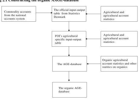
The process of expanding the original database is illustrated in figure 2.1. Starting from the top, the first two levels illustrate the construction of the standard AGE-database without the specific description of organic production.

Initially the agricultural specific input-output table of the Danish economy is constructed. Disaggregating those commodity accounts that are used by Statistics Denmark for constructing the agricultural sector in their official input-output table basically does this. This disaggregation is done by extensive use of various agricultural statistics and sector specific farm accounts.

)LJ&RQVWUXFWLQJWKHRUJDQLF$$*(GDWDEDVH

The third level in fig 2.1 shows that the organic AGE-database is constructed from the existing database. The continued expansion of the organic production and improvement in the collection of primary statistics to cover organic production (the commodity accounts) will determine whether these calculations will move up to the top level of this data construction process.

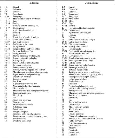
The general AGE-database describes the Danish economy using an industry and commodity aggregation with 50 industries and 56 commodities of which 10 industries and 12 commodities related to the primary agriculture. In the organic version the database is expanded with similar organic sectors and commodities (excluding fur farming) thus leading to 19 primary industries and 23 commodities. Moreover, a number of processing industries are also disaggregated into organic and conventional sectors, resulting in a total of 18 organic industries and 20 organic commodities. The final database thus covers 68 industries and 76 commodities.

7KHFRVWVWUXFWXUHVLQRUJDQLFIDUPLQJ

The cost-structures of the different organic farm sectors are mainly calculated by using the sector specific farm accounts for conventional and organic agricultural, but other sources are

Commodity accounts from the national accounts system

Agricultural and agricultural account statistics

The official input-output table from Statistics Denmark

FOI’s agricultural specific input-output table

The AGE-database

Agricultural and agricultural account statistics

The organic AGE-database

also used to calculate the total production value of each organic product and to collect data on organic prices.

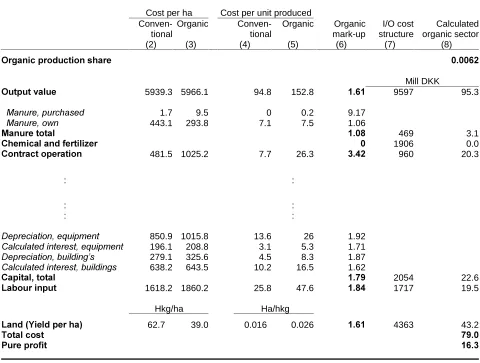
As an example, the calculations for the cereal sector are shown for a sub-set of inputs in table 2.1. Columns two and three show the cost (and output) per hectare of land of producing cereal using conventional and organic technologies respectively. Dividing by the average yield per ha (shown in the last row of the table) results in the cost per unit produced (Hkg) as shown in column four and five. Differences among these figures indicate the differences between conventional and organic production. One unit (Hkg) of conventional output is sold for 94.8 DKK whereas one unit of organic output is sold for 152.8, or 61 percent more. Producing one unit of conventional cereal requires 7.7 and 25.8 DKK worth of contract operations and labour, respectively, whereas producing one unit organic cereal requires 26.3 and 47.6 DKK. Land use also differs. Producing one unit (Hkg) of cereal requires 0.016 hectare of land in conventional farming and 0.026 ha of land in organic farming.

7DEOH Constructing the organic cereal sector of the input-output table: An example

Cost per ha

Cost per unit produced

Conven-tional (2) Organic (3) Conven-tional (4) Organic (5) Organic mark-up (6) I/O cost structure (7) Calculated organic sector (8) 2UJDQLFSURGXFWLRQVKDUH Mill DKK

2XWSXWYDOXH 5939.3 5966.1 94.8 152.8 9597 95.3

0DQXUHSXUFKDVHG 1.7 9.5 0 0.2 9.17

0DQXUHRZQ 443.1 293.8 7.1 7.5 1.06

0DQXUHWRWDO 469 3.1

&KHPLFDODQGIHUWLOL]HU 1906 0.0

&RQWUDFWRSHUDWLRQ 481.5 1025.2 7.7 26.3 960 20.3

: :

: :

: :

'HSUHFLDWLRQHTXLSPHQW 850.9 1015.8 13.6 26 1.92

&DOFXODWHGLQWHUHVWHTXLSPHQW 196.1 208.8 3.1 5.3 1.71

'HSUHFLDWLRQEXLOGLQJ¶V 279.1 325.6 4.5 8.3 1.87

&DOFXODWHGLQWHUHVWEXLOGLQJV 638.2 643.5 10.2 16.5 1.62

&DSLWDOWRWDO 2054 22.6

/DERXULQSXW 1618.2 1860.2 25.8 47.6 1717 19.5

Hkg/ha Ha/hkg

/DQG<LHOGSHUKD 62.7 39.0 0.016 0.026 4363 43.2

7RWDOFRVW

Relating the value per unit produced in the conventional and organic sectors to each other results in the “organic mark-up” shown in column 6. These mark-ups represent the differences in input use in conventional and organic production. Total manure use is 8 percent higher per produced unit in organic production while capital and labour costs are 79 and 84 percent higher, respectively. The capital mark-up is found as a weighted average of the underlying four depreciation and interest categories making up total capital. The reason for this aggregation is that the applied commodity classification is taken directly from the existing AGE-database, which only identifies one capital category. In other cases the sector specific farm accounts variable are more aggregated than in the AGE-database and are therefore used on more than one input commodity.

In the last two columns of table 2.1 the cost structure of organic cereal production is calculated using information on costs in the aggregate cereal sector in the original AGE-database (column 7). The organic cost-structure is calculated by multiplying each aggregate cost component by the organic production share and the organic mark-up for that particular input.

Apart from adjusting for some organic input prices the last column represents the cost-structure of the organic cereal sector. The last row of the column reveals that costs are less than the output value of the sector hence pure profits are made. This pure profit arises because it is assumed that payments to land, labour and capital are equal in organic and conventional production. This assumption can be viewed as a long run or equilibrium requirement to rental rates.

The organic mark-ups for selected industries shown in table 2.2 are represented as percentage changes in input use of producing one unit of organic production compared to one unit of conventional production. In the vegetable sectors, for example, production takes place without the use of chemical, fertilizer or pesticides (-100%). Instead these sectors generally use more of other inputs compared to conventional production (positive percentage changes). For organic cereal production, for example, demanded inputs from contract operations are 2.5 times higher than for conventional production, potato production demands twice as much, while the production of roughage requires just 32 percent more contract operations compared to conventional production.

The table also reveals large variation in the demand for land. Organic cereal production needs 61 percent more land to produce one unit compared to conventional production while the production of organic roughage needs 25 percent more land than its conventional counterpart.

producers generally show moderate percentage changes in their input demand per unit produced compared to conventional cattle production.

At the bottom of the table all the percentage changes are weighted together yielding the percentage change in unit cost. This reveals that the cost of producing one unit of organic cereal is 68 percent higher than cost of producing one unit of the conventional product. In potato production the unit cost is 133 percent higher, while the two tightly connected roughage and cattle sectors show moderate increases in unit costs compared to their conventional counterparts. In other words organic production is generally more resource demanding than conventional production, and thereby leading to relatively higher output prices.

7DEOH2UJDQLFPDUNXSVIRUVHOHFWHGLQGXVWULHVLQSHUFHQW

&HUHDO 3RWDWRHV 5RXJKDJH &DWWOH 3LJV

Seeds for sowing/Roughage 115.0 311.0 15.0 6.1

Concentrates -13.0 56.0

Manure 8.5 120.0 -16.4

Chemistry and fertilizer -100.0 -100.0 -100.0

Pesticides -100.0 -100.0 -100.0

Intermediates 165.0 351.0 55.0 11.0 71.0

Contracts operations 242.0 215.0 32.0 -3.0 72.0

Fuel 57.0 145.0 -9.0 4.0 58.0

Electricity and other energy 120.0 153.0 41.0 14.0 -45.0

Equipment 84.0 126.0 18.0 19.0 62.0

Automobile cost 223.0 343.0 73.0 42.0 135.0

Construction 116.0 150.0 60.0 40.0 211.1

Service 108.5 261.1 37.5 9.6 66.7

Capital 78.7 165.2 24.5 9.2 10.2

Labour 84.0 152.0 -11.0 2.0 93.0

Land 60.5 81.8 25.4

Unit cost _{68.3 132.6 3.8 9.4 63.0}

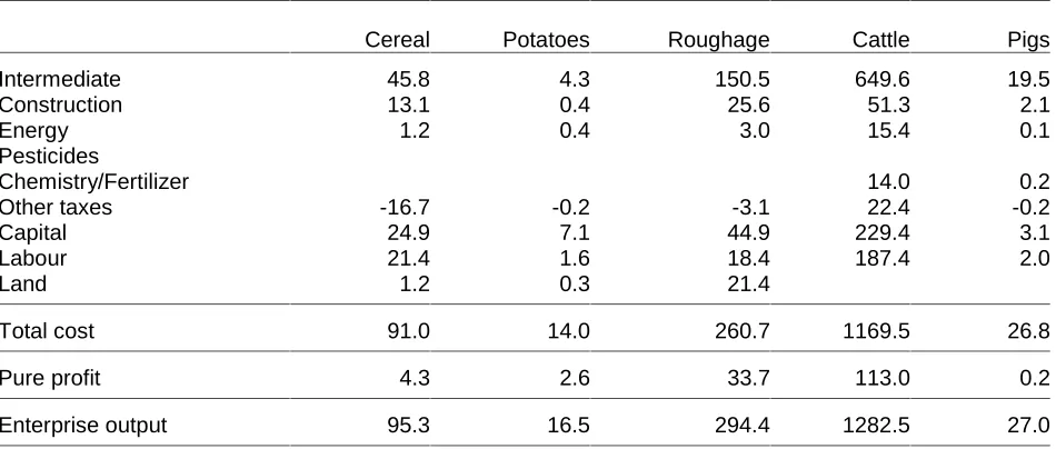
The resulting cost-structure in the AGE-database is given in table 2.3 for selected sectors. A closer inspection shows minor discrepancies for cereals compared with table 2.1. This has to do with the final balancing of the input-output table and the fact that not all organic prices were taken into account in table 2.1.

The table reveals that the cattle (and roughage) sector is the dominant organic production accounting for 79 percent of the total production value. This is hardly surprising given that the cost mark-up relative to conventional production is small, cf. table 2.2 and hence there is a very limited required price difference on the final product.

and capital is paid the same rental in both the conventional and organic sectors. This is a long run requirement for equilibrium, and the pure profit makes it more profitable to produce organically, thus stimulating entry into the industry.

Table 2.3 Aggregated cost structure in selected organic sectors. Mill 1995 DKK

Cereal Potatoes Roughage Cattle Pigs

Intermediate 45.8 4.3 150.5 649.6 19.5

Construction 13.1 0.4 25.6 51.3 2.1

Energy 1.2 0.4 3.0 15.4 0.1

Pesticides

Chemistry/Fertilizer 14.0 0.2

Other taxes -16.7 -0.2 -3.1 22.4 -0.2

Capital 24.9 7.1 44.9 229.4 3.1

Labour 21.4 1.6 18.4 187.4 2.0

Land 1.2 0.3 21.4

Total cost 91.0 14.0 260.7 1169.5 26.8

Pure profit 4.3 2.6 33.7 113.0 0.2

Enterprise output 95.3 16.5 294.4 1282.5 27.0

6XSSO\DQGFRVWVWUXFWXUHLQSURFHVVLQJLQGXVWULHV

So far this section has only dealt with the cost-structure of the primary agricultural sectors. The construction of the database also involves disaggregating the supply structure as well as the disaggregation of the cost-structure in all the processing industries.

There are 9 processing industries that need to be disaggregated (see appendix A). Because appropriate statistics are not available their cost-structures are calculated by assuming the same cost-structures as in the conventional sectors, except for a proportional increase of 5-15 percent on all inputs. The smaller scales of production and the costs of keeping the primary organic products separate explain this.

Statistics on the distribution of organic products for intermediate and final use are also scattered, but it has been possible to construct reliable data for the consumption of organic products. The supplies of primary organic products that are only used in one of the processing industries are easily placed there. For products that are supplied to several users it has been decided to satisfy the calculated consumption and the use in the processing industry (if any) first. The remainder is then distributed to other uses according to the relative distribution in the conventional supply. The latter consists mainly of private and public services, which includes restaurants, staff restaurants and public food services.

7KH$$*(PRGHO

There are five types of agents in the AAGE ($gricultural $pplied *eneral (quilibrium) model: industries, capital creators, households, governments, and foreigners. The current database of the model identifies 68 industries producing 76 commodities (see appendix A). For each industry there is an associated capital creator. The capital creators each produce units of capital that are specific to the associated industry. There is a single representative household and a single government sector. Finally, there are foreigners, whose behaviour is summarised by export demand curves for Danish products, and by supply curves for imports.

7KHQDWXUHRIPDUNHWVDQGSULFHV

AAGE determines supplies and demands of commodities through optimising behaviour of agents in competitive markets. Optimising behaviour also determines industry demands for labour and capital.

The assumption of competitive markets implies equality between the producer’s price and the marginal cost in each industry. Demand is assumed to equal supply in all markets other than the labour market (where excess supply conditions can hold). The government intervenes in markets by imposing sales taxes on commodities. This places wedges between the prices paid by purchasers and prices received by the producers. The model recognises margin commodities (e.g. retail trade and freight) that are required for each market transaction (the movement of a commodity from the producer to the purchaser). The costs of the margins are included in purchasers’ prices.

'HPDQGVIRULQSXWVWREHXVHGLQWKHSURGXFWLRQRIFRPPRGLWLHV

AAGE recognises two broad categories of inputs: intermediate inputs and primary factors. Firms in each industry are assumed to choose the mix of inputs, which minimises the costs of production for their level of output. They are constrained in their choice of inputs by nested production technologies (see appendix B). For the land-using industries (see appendix A), AAGE specifies nested substitutions between:

(a) capital, labour, energy and herbicides (CLEH); (b) land, fertiliser and insecticides (LFI);

(c) CLEH and LFI (CLEHLFI); and

(d) CLEHLFI and an aggregate of remaining intermediate inputs

For non-land using industries substitution is allowed between capital, labour and energy (CLE) and between CLE and aggregate non-energy intermediate inputs.

+RXVHKROGGHPDQGV

'HPDQGVIRULQSXWVWRFDSLWDOFUHDWLRQDQGWKHGHWHUPLQDWLRQRILQYHVWPHQW

Capital creators for each industry combine inputs to form units of capital. In choosing these inputs, they cost minimise subject to technologies similar to that used for current production; the only difference being that they do not use primary factors. The use of primary factors in capital creation is recognised through inputs of the construction commodity.

*RYHUQPHQWVGHPDQGVIRUFRPPRGLWLHV

The government demands commodities. In AAGE, there are several ways of handling these demands, including: (i) endogenously, by a rule such as moving government expenditures with household consumption expenditure or with domestic absorption; (ii) endogenously, as an instrument which varies to accommodate an exogenously determined target such as a required level of government deficit; and (iii) exogenously. In the computation in this paper government demand changes follow household consumption expenditures.

)RUHLJQGHPDQGLQWHUQDWLRQDOH[SRUWV

Two categories of exports are defined: traditional, which are the main exported commodities, and non-traditional. Traditional export commodities face individual downward-sloping foreign demand schedules. The commodity composition of aggregate non-traditional exports is treated as a Leontief aggregate. Total demand is related to the average price via a single downward-sloping foreign demand schedule. Contrary to many conventional agricultural products all organic products are assumed to be traditional export commodities.

'HPDQGIRUIRUHLJQLPSRUWV

For all industries, AAGE includes the standard Armington specification for imported and domestically produced inputs. This assumes that users of a given commodity regard the domestic and the imported varieties of this commodity as imperfect substitutes. The Armington assumption is also used in input demands for industry investment and in household demands for consumption.

&RPSXWLQJVROXWLRQVIRU$$*(

6FHQDULRV

A baseline is constructed to introduce all ongoing policy developments and known shocks to the economy so as to ensure that the policy shocks are undertaken in an economy where all known developments and shocks are accounted for.

We introduce four alternative scenarios. First, the SUHIHUHQFH scenario is introduced, where domestic and foreign consumers of Danish products change their preferences in favour of organic products. The SUHIHUHQFH scenario is then compared with three policy scenarios in the absence of the assumed consumer preference change.

The first two policy experiments (6XE$ and 6XE%) use subsidies to agricultural land in the organic sectors to induce a movement of land into organic production to achieve a positive environmental effect. The first policy experiment (6XE$) is designed so as to achieve the same share of organic land as obtained in the SUHIHUHQFH scenario. This does not automatically result in the same reduction in the use of harmful inputs. Therefore, the second policy experiment (VXE%) uses such subsidies to achieve the same effects on the environmental indicators as obtained in the SUHIHUHQFH scenario.

The third policy experiment (7D[) imposes environmental taxes on fertilizer and pesticide use to achieve the same effects on the environmental indicators as in the SUHIHUHQFH scenario and 6XE%. The idea is to compare two different policy instruments, namely subsidies to land and input taxes that achieve the same effect on the use of environmentally harmful inputs (fertilizers and pesticides).

The policy implication would be to choose the policy that achieves the same goal at the lowest cost to society.

([SHFWHGUHVXOWVIURPWKHDQDO\VLV

The introduced subsidies lower the cost of using land in the organic sectors (the purchasers’ price of land is reduced), thereby yielding pure profit in the organic sector and hence stimulating entry to organic production. This leads to an increase in the demand for land, with an upward pressure on the basic price of land as a result. The subsidy also changes the relative price of land thus leading to a substitution effect resulting in an extensification of organic production. In other words, more land and less capital and labour is used per produced unit.

Subsidies are thus expected to increase the production of organic products but are also expected to lead to an extensification of organic production. The exact extent of these two effects depends on how demand for organic products is affected.

unit cost requires a higher product price if profits are to remain unchanged. Yet a higher product price tends to lower demand. A decline in production releases resources to be used in other sectors of the economy and tends to lower the prices and required rental of these resources because of the increase in supply. Since the taxes are levied on conventional land- using sectors and land is only used in the agricultural sectors (whereas labour, capital and other inputs are also used in the rest of the economy), land is expected to bear the greatest burden of the levied taxes in the form of lower returns to land. Relative lower returns to land will also results in a substitution effect where the land-using sectors will substitute other inputs, especially capital and labour, for land.

5HVXOWV

This section presents selected results of the calculated scenarios, including the effects on production, exports, consumption, land and labour use and the environmental indicators. Section 5 concludes by presenting the macroeconomic impacts. The presentation focuses on the results for the primary agricultural and associated processing sectors. Since the main issue addressed is the comparison of the results from applying the two different policy instruments this will be the focus of the analysis4.

3URGXFWLRQDQGRUJDQLFODQG

In the EDVHOLQH aggregate organic production in the primary agricultural sector increases by an average of 5 pct. p.a. This results in 5 pct. of total land being used for organic production (Fig 5.1) and almost 6 pct. of the total production volume arising from organic production.

Fig 5.1 also shows that the assumed changes in SUHIHUHQFH scenario have significant effects on both the organic share of land (8.7 pct.) and it’s share of the total agricultural production volume (10.7 pct). Aggregate organic production increases by 84.4 pct whereas conventional production falls by 4.7 pct. (see table C.1). The last three scenarios are to be compared with the SUHIHUHQFH scenario since scenario 6XE$ results in the same share of land allocated to organic production whereas scenarios 6XE% and 7D[ result in the same reduction in the use of nitrogen and pesticides.

The land subsidies lower the purchaser’s price of land, thereby lowering the unit price of organic products and stimulating demand. Lower land prices also stimulate a substitution of all other inputs in favour of land thus leading to an extensification of organic production. Comparing with the SUHIHUHQFHscenario it is clear that it is the land substitution effect that dominates in 6XE$ and 6XE%. In scenario 6XE$ and 6XE% the share of land are higher than or equal to the land shares in the 3UHIHUHQFH scenario, whereas the increase in production is much smaller (production increases by 17 pct. (6XE$) and 18 pct. (6XE%) compared to 84 in the SUHIHUHQFH scenario, see table C.2 in appendix C.

)LJ7KHRUJDQLFVHFWRU¶VVKDUHRIWKHWRWDODJULFXOWXUDOSURGXFWLRQYROXPHDQGODQG XVDJH

3HUFHQW

%DVHOLQH 3UHIHUHQFH 6XE$ 6XE% 7D[

3URGXFWLRQ /DQG

Note: Details can be found in appendix table C.1

In the last scenario (7D[), environmental taxes are imposed on inputs used only in the conventional sector in a magnitude that insures the same aggregate effect on the input of nitrogen and pesticides as in the SUHIHUHQFH scenario and 6XE% (see fig 5.3 and 5.4 below).

In the SUHIHUHQFH scenario it is the movement of land into organic production that achieves the aggregate reduction in the use of nitrogen and pesticides. In fact, conventional farmers use these chemicals more intensively in this scenario due to a substitution effect generated by a slight increase in land prices.

2UJDQLFFRQVXPSWLRQDQGH[SRUWV

The representative household determines its composition of total consumption to maximize a given utility function. In the top nest, the consumer system determines the composition of a number of aggregate goods by a Stone-Geary linear expenditure system. The expenditure system identifies four broad food commodities; Bread and flour, Meat, Dairy and Other5. Beneath this nest a CES function determines the composition of organic and conventional products using econometrically estimated elasticities6. At the bottom of the nesting structure, a CES function controls the domestic and foreign composition of all commodities. In the CES nest between conventional and organic products a “twist” variable is built in to allow for cost-neutral changes in the composition of organic and conventional consumption.

Consumption decisions are influenced by changes in income and relative prices, but in both the EDVHOLQH and the SUHIHUHQFH scenario, the exogenous twist variable also plays an important role. It is this variable that is shocked and the results show that most of the changes in organic consumption directly reflect the shock to the twist variable.

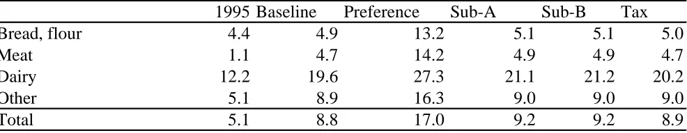
Changed relative prices also affect the consumption decision of the consumer, but the resulting consumption shares of organic products are in both the baseline and in the preference scenario mostly explained by the assumed changes in preferences, i.e. the exogenous shock to the twist variable explained above. In the preference scenario the consumption of organic dairy products amounts to 27 percent of total consumption in this category while for the other three categories, organic consumption amounts to around 15 percent. At the aggregate level, organic food consumption amounts to 17 percent of the total (table C.3 in appendix) in this 3UHIHUHQFH scenario.

When compared to the EDVHOLQH results (fig 5.2), it is apparent that the consumption decisions are not markedly influenced by the introduction of the subsidies and taxes in the last three scenarios. As explained earlier, changes in consumption are explained primarily by income changes and consumers’ responsiveness to changes in relative prices. In the last three scenarios only moderate effects are seen compared with the EDVHOLQH results even though all three experiments change the price structure in favour of organic products and higher elasticities in the demand for organic products7. The reason is that the large price effect is seen most directly on the primary product. When the products have been processed, the price effect is smaller due to the fact that the primary product only accounts for a fraction of total costs in the processing industries.

5 _{Mostly vegetables.} 6

Wier and Smed (2000)

)LJ2UJDQLFFRQVXPSWLRQVKDUHVYROXPHLQGH[

3HUFHQW

%DVHOLQH 3UHIHUHQFH 6XE$ 6XE% 7D[

%UHDGIORXU 0HDW 'DLU\ 2WKHU

In the %DVHOLQH the share of organic exports is calculated to increase from practically zero in the initial situation to somewhere around one to six percent. In the 3UHIHUHQFH scenario there is an assumed change in foreigners’ demand curves in favour of organic products at the given prices. Meat exports declines even though the demand curve is shifted. This is a result of the increased domestic demand pressuring prices upwards, thereby resulting in lower export demand. In other words, the price effect dominates the shift in the export demand schedule. As with the domestic consumption, only moderate effects are seen in the last three scenarios and for the same reasons. For dairy products stronger effects are seen due to an assumed higher elasticity in the export demand function.

7DEOH2UJDQLFH[SRUWVKDUHVYROXPHLQGH[

3HUFHQW

%DVHOLQH 3UHIHUHQFH 6XE$ 6XE% 7D[

%UHDGIORXU 0HDW 'DLU\ 2WKHU

Bread, flour is an aggregate of 8 commodities meat and other is an aggregate of 6 and 3 commodities.

Results for both domestic consumption and exports show that both land subsidies and the environmental taxes affect demand. Yet keeping in mind that either land use or the effect on the environmental indicators is the same as in the SUHIHUHQFH scenario (depending on which scenario we are examining) it is evident that these policy instruments can affect land use and input choices, but they do relatively little to overall demand and production.

(QYLURQPHQWDOLQGLFDWRUV

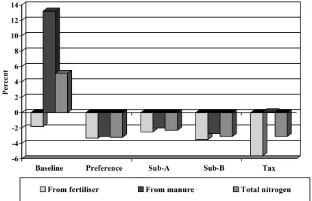
The baseline shows a decrease in the use of pesticides (fig 5.4) because of an increase in the taxes on pesticides during the base case period. The use of nitrogen, on the other hand, increases during the %DVHOLQH(fig 5.5). This is mainly due to increased production of manure (pig production increases by more than 30 percent).

In the 3UHIHUHQFH scenario, the movement of land into organic production results in decreases in both the use of pesticides (fig 5.4) and nitrogen (fig 5.5).

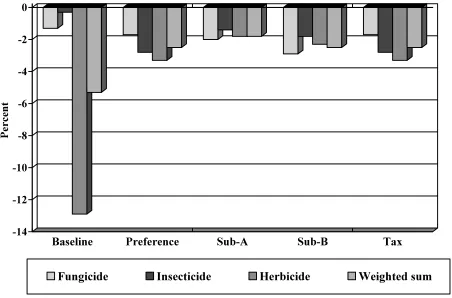
Fig 5.4 Changes in the use of pesticides

3HUFHQW

%DVHOLQH 3UHIHUHQFH 6XE$ 6XE% 7D[

)XQJLFLGH ,QVHFWLFLGH +HUELFLGH :HLJKWHGVXP

Introducing subsidies to organic land that insure the same organic area as in the 3UHIHUHQFH scenario is not enough to achieve the same reduction in the use of pesticides (6XE$). As fig 5.4 shows the decrease is less than 2 percent measured by the weighted sum. The reason is that the use of land in conventional production changes to a more pesticide intensive allocation than was the case in the SUHIHUHQFH scenario. In scenario 6XE% these subsidies to organic land are increased to attract more land, thereby resulting in the same reduction in the weighted sum of pesticides as in the SUHIHUHQFH scenario8. In the 7D[ scenario taxes are introduced to exactly match the reduction in the 3UHIHUHQFH scenario. Total pesticide use falls by 2.5 percent in this scenario.

As with pesticides, introducing subsidies to organic land that insure the same organic area as in the 3UHIHUHQFH scenario, is not enough to achieve the same reduction in the use of nitrogen (6XE$). The decrease is slightly more than 2 percent (fig 5.5). The reason is that the allocation of land in conventional production changes to a situation where more fertilizer is used than was the case in the 3UHIHUHQFH scenario. In scenario 6XE% these subsidies to organic land are increased to attract more land, thereby resulting in the same reduction in the use of nitrogen. In the 7D[ scenario environmental taxes are introduced that result in the same reduction in the total use of nitrogen whereas the composition is quite different. In the 7D[ scenario the total change is a result of a decrease in the use of

fertilizers. In fact, there is a small increase in the use of manure due to a slight increase in the animal production9.

Fig 5.5 Changes in the use of nitrogen

3HUFHQW

%DVHOLQH 3UHIHUHQFH 6XE$ 6XE% 7D[

)URPIHUWLOLVHU )URPPDQXUH 7RWDOQLWURJHQ

(PSOR\PHQW

In the %DVHOLQH the total number of full time workers in primary agriculture falls by almost 13,000 persons (table 5.1). This is mainly due to structural development and increases in labour productivity. In the 3UHIHUHQFH scenario the demand shift from conventional to organic commodities is also reflected in the employment result. The total number of employed in the conventional sectors thus falls by 3,211 persons while employment in the organic sectors increases by 3,100 fulltime employees. Thus net-employment in the primary agricultural sectors falls by just 111 persons.

Both subsidy scenarios work in the same way, with the strongest effects being in 6XE%. Employment in the conventional sectors falls by almost 1,200 persons in this scenario while 600 more persons are employed in the primary organic sectors. In the 7D[ scenario the effects are more moderate, with 163 persons leaving the conventional sectors and 179 entering the primary organic sectors.

In the two subsidy scenarios it is mainly the movement of land that explains the results. Land moves out of conventional production resulting in less production and less use of labour. The released land moves into organic production, but since demand does not follow the inflow of land, this results in an extensification effect in organic production: all other inputs are to some extent substituted by land in the organic production.

In the 7D[ scenario, the taxes result in both lower conventional production and thereby also less demand for inputs of land, labour and capital, but also in a substitution effect where taxed inputs are substituted with other inputs (especially labour). The result is a more labour intensive conventional production. For the organic producers the 7D[ scenario first of all results in lower land prices, pressuring the unit prices to decline and thus stimulating demand and production. Yet the lower land prices also result in a minor substitution effect between land and other inputs. As can be seen from table 5.1 the 7D[scenarioresults in a minor net increase in the use of labour in the primary agricultural sector.

Table 5.1 Employment, number of fulltime persons

Deviation from Baseline

1995 Baseline Preference Sub-A Sub-B Tax

Primary, conventional 84978 71521 -3211 -961 -1198 -163

Primary, organic 2837 3608 3100 547 600 179

7RWDOSULPDU\DJULFXOWXUH

Processing, conventional 33197 25815 -1281 -640 -865 -12

Processing, organic 582 819 803 171 186 59

Total 121594 101764 -589 -883 -1278 63

0DFURHFRQRPLFFRQVHTXHQFHV

The macroeconomic consequences of all four preference and policy scenarios are small. The effect on real GDP varies between a fall of 0.01 percent and 0.08 percent, i.e. the consequences for the economy as a whole are small. But the magnitude of change in the different scenarios does reveal that there are differences in the relative cost to society.

In the preference scenario real GDP and consumption fall by 0.07 and 0.14 percent respectively, but these declines can’t be interpreted as a situation in which society is worse off since they are a result of changed consumer preferences. If consumers change their preferences in favour of a product that is produced at a higher cost, (thus lowering the total real consumption potential) it must be because they are better off by this choice. In other words, the new consumption bundle yields a higher utility to the consumer.

result than increasing capital stocks in industries with relatively large investment/capital ratios.

The three other scenarios, on the other hand, are a result of policy intervention, and the results must be interpreted as costs to society. If these scenarios result in the same effects on the policy objective, these figures may also guide us to the most cost-effective policy of those analysed. Finally, a policy instrument should only be used if the benefit to society is higher than the cost. In this context it should be noted that all potential benefits are not a part of this analysis.

Table 5.1 Macroeconomic consequences.

1995-Level Preference Sub-A Sub-B Tax Billion DKK Million DKK

Percent

Million DKK Percent

Million DKK Percent

Million

DKK Procent

Real GDP 1037.7 -728 -0.07 -617 -0.06 -859 -0.08 -128 -0.01 Real private consumption 511.1 -740 -0.14 -392 -0.08 -557 -0.11 40 0.01 Real public consumption 260.3 -360 -0.14 -190 -0.08 -271 -0.11 19 0.01 Real investments 189.3 82 0.04 -190 -0.10 -272 -0.15 -17 -0.01

Real stocks 39.3 0 0.00 0 0.00 0 0.00 0 0.00

Real exports 296.0 320 0.11 171 0.06 194 0.06 -159 -0.05 Real imports 258.3 -22 -0.01 -7 0.00 -96 -0.04 45 0.02

Real capital stock -0.04 -0.09 -0.13 -0.01

GDP deflator -0.13 -0.14 -0.18 -0.03

Consumer price index -0.08 -0.09 -0.13 -0.01

-0.12 -0.16 -0.22 -0.05

Terms of Trade -0.06 0.01 0.01 0.02

Nominal wage rate -0.25 -0.33 -0.44 -0.11

Price of agricultural land 0.34 9.55 14.07 -17.75

Price of investment goods

Comparing the two subsidy scenarios (6XE$and 6XE%), it is clear that the cost in terms of real GDP is higher the more land is shifted into organic production. The reason for this is of course that more land is being used in a less productive sector, thus lowering the total production possibility of the economy. Lower productivity results in lower returns to capital and labour and thus also lower income and lower consumption possibilities. For the agricultural sector as a whole though, the subsidies increase the returns to land resulting in increase land price of (9.6 and 14.1 percent).

The tax scenario results in exactly the same reduction in the total use of pesticides and nitrogen as subsidy scenario B (6XE%) but at a lower cost. In terms of GDP the cost of the 7D[ scenario amounts to 0.01 percent of GDP. Achieving the same reduction in nitrogen and pesticide use by using subsidies (6XE%) costs almost seven times more.

different policy instruments. Imposing environmental taxes that affect the majority of farmers turns out to be the most cost-effective instrument.

There is a small increase in real consumption in the 7D[ scenario. This is not a generic result of taxing pesticides and fertilizers. Real consumption increases because the income loss in this scenario is so small that the falling consumer prices allow for this small increase in real consumption. If the scenario was specified with higher taxes or taxes that applied to a larger part of the economy, the income loss would dominate and result in a fall in real consumption. Real public spending also increases. This is a result of the model closure where the percentage change in real public spending is set equal to the change real private consumption.

The consequences of the scenarios for landowners are also shown in table 5.1. In the subsidy scenarios land prices increase while in the 7D[ scenario the price falls.

&RQFOXGLQJUHPDUNV

This paper has analysed the economy wide implication of two different policy instruments targeted at reducing the overall use of pesticides and fertiliser. The analysis shows that in absence of consumer preference changes, subsidies (6XE$ and %) can be used effectively to change the relative profitability between organic and conventional production, thereby resulting in a shift of land into organic production of the same magnitude as that resulting from changed consumer preferences. Yet although the aggregate land use is the same, the increase in production is almost five times higher in the 3UHIHUHQFH scenario compared with the 6XE% scenario. The results also show that subsidising the organic sectors leads to a situation in which the conventional sectors use pesticides and fertilisers more intensively.

The implications for land prices are also different in the two scenarios. While the land subsidies result in land price increases and thus higher returns to land owners, the 7D[ scenario results in lower prices of land.

Even though the macroeconomic consequences of the analysed scenarios are small, the relative magnitudes are clear. In terms of real GDP, the cost of reducing the aggregate use of fertilizers and pesticides is seven times higher when using subsidies to organic farming compared to taxing the use of these inputs.

If society is concerned about the overall use of environmentally harmful inputs these inputs should be taxed or regulated in a similar way. The size of the organic sector should be determined by the consumers’ willingness to pay.

5HIHUHQFH

Adams, P.D (2000), “Dynamic-AAGE: A Dynamic Applied General Equilibrium Model of The Danish Economy Based on AAGE and MONASH models”, Report number 115. Available from the Danish Research Institute of Food Economics.

Frandsen and Jacobsen (1999 a) Analyser af de samfundsøkonomiske konsekvenser af en omlægning dansk landbrug til økologisk produktion, SJFI working paper no. 5/1999. Available from the Danish Research Institute of Food Economics.

Frandsen and Jacobsen (1999 b) Analyser af de sektor- samfundsøkonomiske konsekvenser af en reduktion i forbruget af pesticider i dansk landbrug, SJFI report no. 104. Available from the Danish Research Institute of Food Economics.

The Bichel Committee 1999, Report from the Sub-committee on Production, Economics and Employment. The Danish Environmental Protection Agency. Available electronically from www.mst.dk

Pearson, K.R. (1998), “Automating the Computation of Solutions of Large Economic Models”, Economic Modelling, Vol. 7, pp. 385-395.

Harrison W. Jill and K.R. Pearson (1996), "Computing solutions for Large General Equilibrium Models Using GEMPACK", Computational Economics, Vol 9, pp. 83-127.

Wier, M & Smed, S. (2000), )RUEUXJ DI ¡NRORJLVNH I¡GHYDUHU 'HO 0RGHOOHULQJ DI HIWHUVS¡UJVOHQ. Danmarks Miljøundersøgelser, 186 s. Faglig rapport fra DMU, nr. 319.

Jacobsen, Brian H. (2002), Reducing Nitrogen Leaching in Denmark and the Netherlands Administrative regulation and costs, Poster Paper for the Xth EAAE Conference in Zaragoza, 2002.

Jacobsen, Lars-Bo (2001). 3RWHQWLDOHW IRU ¡NRORJLVN MRUGEUXJ ± 6HNWRU RJ

VDPIXQGV¡NRQRPLVNH EHUHJQLQJHU. Rapport nr. 121. Statens Jordbrugs og

Fiskeriøkonomiske Institut.

Kristensen and Thamsborg eds. (2000) Sundhed, velfærd og medicinanvendelse ved omlægning til økologisk mælkeproduktion. rapport 6/2000 Forskningscenter for Økologisk Jordbrug.

Jensen et.al. 2001 Økologiske fødevarer og menneskets sundhed – Rapport fra vidensyntese udført i regi af Forskningsinstitut for Human Ernæring, KVL, rapport 14/2001 Forskningscenter for Økologisk Jordbrug.

Langer et al. 2002 Omlægning til økologisk jordbrug i et lokal område – Scenarier for natur, miljø og produktion, rapport 12/2002 Forskningscenter for Økologisk Jordbrug.

$SSHQGL[$

Table A.1 Industries and commodities in Organic-AAGE.

Industries Commodities

*# 1-2 Cereal * 1-2 Cereal

*# 3-4 Oil seeds * 3-4 Oil seeds *# 5-6 Potatoes * 5-6 Potatoes *# 7-8 Sugerbeets * 7-8 Sugerbeets *# 9-10 Roughage * 9-10 Roughage * 11-12 Meat cattle and milk producers * 11-12 Meat cattle

* 13-14 Pigs * 13-14 Milk

* 15-16 Poultry * 15-16 Pigs 17 Hunting and fur farming, etc. * 17-18 Poultry

*# 18-19 Horticulture 19 Hunting and fur farming, etc. 20 Agricultural services, etc. * 20-21 Horticulture

21 Forestry 22 Agricultural services, etc.

22 Fishing 23 Forestry

23 Extraction of coal, oil and gas 24 Fishing

* 24-25 Cattle-meat products 25 Extraction of coal, oil and gas * 26-27 Pig-meat products * 26-27 Cattle-meat products * 28-29 Poultry-meat products * 28-29 Pig-meat products

30 Fish products * 30-31 Poultry-meat products * 31-32 Processed fruit and vegetables 32 Fish products

33 Processed oils and fats * 23-34 Processed fruit and vegetables * 34-35 Dairy products 35 Processed oils and fats * 36-37 Starch, chocolate products, etc. * 36-37 Dairy products

* 38-39 Bread, grain mill and cakes * 38-39 Starch, chocolate products, etc. * 40-41 Bakery shops * 40-41 Bread, grain mill and cakes * 42-43 Sugar factories and refineries * 42-43 Bakery shops

44 Beverage production * 44-45 Sugar factories and refineries 45 Tobacco manufacture * 46-47 Beverage production 46 Textile, wearing apparel and leather 48 Tobacco manufacture

47 Manufactured wood and glass products 49 Textile, wearing apparel and leather 48 Paper products and publishing 50 Manufactured wood and glass products 49 Oil refinery products 51 Paper products and publishing 50 Basic chemicals 52 Oil refinery products 51 Fertiliser 53 Basic chemicals 52 Agricultural chemicals nec 54 Fertiliser

53 Non-metallic building material 55 Agricultural chemicals nec 54 Metal products 56 Non-metallic building material

55 Machinery and non-transport equipment 57 Metal products

56 Transport equipment 58 Machinery and non-transport equipment 57 Electricity 59 Transport equipment

58 Gas 60 Electricity

59 Steam and hot water 61 Gas

60 Construction 62 Steam and hot water 61 Motor vehicles service 63 Construction 62 Wholesale trade 64 Motor vehicles service 63 Retail trade 65 Wholesale trade 64 Freight transport 66 Retail trade 65 Financial and property services 67 Freight transport

66 Transport and communication services 68 Financial and property services 67 Public services 69 Transport and communication services 68 Dwelling ownership 70 Public services

71 Dwelling ownership 72 Coal imports

73 Manure

74 Fungicide

75 Insecticides

76 Herbicide

$SSHQGL[%1HVWLQJVWUXFWXUH

Produktion

Capital, Labour, Energy, Fertiliser, Pesticides, Land and Intermediate Inputs

Taxes Special Imports

Capital, Labour, Energy,

Fertiliser, Pesticides, Land Intermediate Inputs

Capital, Labour, Energy and Herbicides

Herbicides Capital, Labour and _Energy

Energy _{Capital and Labour}

Labour Capital

Fertiliser, Fungicides, Land and Insecticides

Fertiliser and Fungicides Land

Fungicides

Fertiliser Fertiliser

Manure

Fertiliser, Fungicides

and Land Insecticides

$SSHQGL[&'HWDLOHGUHVXOWVWDEOHV

Table C.1 Organic share of land and value of production

1995 Baseline Preference Sub-A Sub-B Tax

Production value 3.5 5.0 9.5 5.5 5.6 5.0

Production volumes 3.5 5.8 10.7 6.9 7.0 6.1

Agricultural land 2.8 4.8 8.7 8.7 10.2 5.3

Table C.2 Changes in production, percentage changes

Baseline Pct.pa. Preferences Sub-A Sub-B Tax

Conventional productio 20.6 1.3 -4.7 -2.3 -3.0 -0.4

Organic production 107.1 5.0 84.4 17.1 18.4 5.9

Total 23.6 1.4 -0.2 -1.3 -1.9 -0.1

Table C.3 Organic consumption shares.

Other is mainly vegetable.

1995 Baseline Preference Sub-A Sub-B Tax

Bread, flour 4.4 4.9 13.2 5.1 5.1 5.0

Meat 1.1 4.7 14.2 4.9 4.9 4.7

Dairy 12.2 19.6 27.3 21.1 21.2 20.2

Other 5.1 8.9 16.3 9.0 9.0 9.0