by
Peter J, Forrester
Thesis submitted for the Degree of Doctor
of Philosophy at the Australian National
University
1985
and integrals arising in generalizations of some known exactly solved models in statistical mechanics.
In Part I we study classical Coulomb systems with the logarithmic potential (leg-gases). The multidimensional integrals representing the partition function and correlation functions of three new log-gas systems are evaluated. These systems are (for a single special value of the coupling constant) a two-component log-gas on the circle with charge ratio 1:2, a two-component "generalized" plasma on the circle, and a two-dimensional model of the metal-electrolyte boundary. In each case the thermodynamic limit is obtained, and the models are studied from a physical viewpoint. This latter study is mostly concerned with the verification and/or formulation of sum rules for these systems. As well as their interpretation as Coulomb systems,the Boltzmann factors of both the log-gases and generalized plasmas have interpretations as ground state wavefunctions for certain quantum many body problems. This analogue is used to check and/or formulate sum rules for the quantum system. Furthermore, for the two-component log-gases we consider the zero-temperature statistical mechanics, in
particular the equilibrium configurations and corresponding energies. In Part II we study the restricted eight-vertex solid-on-solid
model corresponds to the case s = 1 , r = 5 . Using the corner transfer matrix technique, expressions in terms of combinatorial sums are then obtained for the local height probabilities in the large but finite lattice. A generalization of Schur’s proof of the Rogers- Ramanujan identities is then used to transform these expressions into a form suitable for taking the infinite lattice limit. This allows us to express the combinatorial sums as modular forms, and thus obtain generalizations of the Rogers-Ramanujan identities. Furthermore, when calculating the normalizations of these probabilities, we encounter generalizations of the so called "sums-of-products" identities: summation formulae for special combinations of the modular forms occuring in the Rogers-Ramanujan identities.
A crucial tool used in Part II is the corner transfer matrix technique. In Part III we generalize the ideas underlying the corner transfer matrices to three dimensions. This allows a variational approximation for three-dimensional lattice models to be formulated. To test the accuracy of the approximation, it is first used to obtain
that research. Most commonly the answer is that they came from the experience of previous investigations by the researcher into similar problems. An exception is the source of the main ideas and choice of subject matter contained in the typical scientific doctrate thesis. There that source is nearly always the supervisor of the thesis.
The topics of Parts II and III of this thesis are the ideas of my Ph.D. supervisor, Professor R.J. Baxter. In Part III we developed the ideas together, while in Part II we worked in collaboration with Professor G.E. Andrews of the University of Pennsylvania, who is an expert in combinational number theory.
The research in Part I is a continuation of ideas developed in
a study of classical Coulomb systems began in my M.Sc. thesis at Melbourne University in 1982 under the supervision of Dr. E.R. Smith. Throughout the duration of my research into this topic I have been in contact with Professor B. Jancovici of l'Universite de Paris-Sud, centre d'Orsay, culminating in a three month visit to Orsay during 1985. Professor Jancovici provided valuable advice and comments on the physics of my mathematical results.
Thus, for ideas and collaboration, I thank Professors Baxter, Jancovici and .Andrews.
via eleven separate publications. Here we list those publications, together with the corresponding chapter(s) of the thesis.
Chapter 1: P.J. Forrester, 'An exactly solvable two-component classical Coulomb system', J. Austr. Math. Soc. Series B 26 (1984),
119-128.
P.J. Forrester, 'Interpretation of an exactly solvable two-component plasma', J. Stat. Phys. _35 (1984), 77-87.
Chapter 2: P.J. Forrester and J.B. Rogers, 'Electrostatics and the zeros of the classical polynomials', to appear SIAM J. Math. .Analysis.
Chapter 3: P.J. Forrester, 'Analogues between a quantum many body problem and the log-gas', J. Phys.A: Math. Gen. YJ_
(1984), 2059-2067.
Chapter 4: P.J. Forrester and B. Jancovici, 'Generalized plasmas and the anomalous quantum Hall effect', J. Physique Lett. 45 (1984) , L583-L589.
Chapter 5: P.J. Forrester, 'The two-dimensional one-component plasma at P = 2 : metallic boundary', to appear J. Phys. A.
A. Alastuey, L. Blum, P.J. Forrester, B. Jancovici and M.L. Rosinberg, 'Comment to "The ideally polarizable
type identities', J. Stat. Phys. (1984), 193-266.
P.J. Forrester and R.J. Baxter, 'Further exact solutions of the eight-vertex SOS model and generalizations of the Rogers-Ramanujan identities', J. Stat. Phys. 38
(1985),435-472.
Chapter 9: R.J. Baxter and P.J. Forrester, 'A variational approximation for cubic lattice models in statistical mechanics',
J. Phys. A: Math. Gen. 17 (1984), 2675-2685.
PART I
1. An exactly solvable two-component plasma
1.1 From random matrices to the one-component log-gas 3
1.2 The two-component plasma 5
1.3 Evaluation of the partition function 7
1.4 A local limit theorem and the evaluation of the free
energy 12
1.5 The excess free energy of mixing 15
1.6 The two particle correlations 16
1.7 Verification of the sum rules 20
1.8 Discussion 22
2. Equilibrium positions of the two-component plasma 2.1 Stieltjes, electrostatics and the zeros of the classical
polynomials 26
2.2 Two impurities on the circle 26
2.5 The thermodynamic limit: unit charges about an impurity 31
2.4 A single impurity on the line 33
2.5 Crystal lattices on the circle 57
2.6 Energy of crystal structures 41
5. A quantum many body problem
?
3.1 From the one-component log-gas to the 1/r“ potential
Schrödinger equation 44
3.2 The single species quantum system 45
3.3 The t-species quantum system 50
4. Generalized plasmas and the anomalous quantum Hall effect 4.1 Another quantum many body problem, classical plasma
analogy 60
4.2 The two-dimensional generalized plasma 61
4.3 The one-dimensional generalized plasma 64
4.4 A one-dimensional solvable model 65
5. The two-dimensional one-component plasma at r = 2: metallic boundary
5.1 Analogies between matrix ensembles and the
two-dimensional one-component plasma 75
5.2 Evaluation of the grand canonical partition function and
the N-particle correlations 75
5.5 Zero background charge density: charges near a metal wall 85
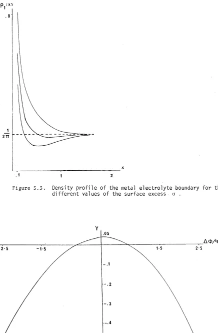
5.4 The metal-electrolyte boundary SS
5.5 The ideally polarizable interface: another approach to the
metal-electrolyte boundary 95
Appendix 99
References for Part I 101
PART II
6. The local height probabilities P a
6.1 More classical analysis, statistical mechanics interplay 105 6.2 The eight-vertex model and an "equivalent"
solid-on-solid model 104
6.6 The ground states
6.7 P for the large but finite lattice a
Appendix
7. Evaluation of the probabilities P^
7.1 The combinatorial sums D and the Rogers-Ramanujan m
identities
7.2 Gaussian polynomials
7.5 The P^ in terms of the Gaussian polynomials 7.4 The large-m limit in Regime IIIr , y ^ r-1
b 7.5 The large-m limit in Regime II
b 7.6 Number of ground states from the P^
7.7 The normalization constant and sums-of-products identities 7.8 Final results
Appendix
8. Critical behaviour
8.1 Multicriticality in the restricted eight-vertex SOS model 8.2 The P^ in terms of the original variables
8.5 Expansions of the P around criticality for the physical regimes
8.4 Expansions of the P around criticality for the unphysical a
regimes 8.5 Free energy
119 122 126 155 157 159 144 149 161 162 169 172 178 178 184 186 188
models
9.1 3eyond the corner transfer matrices 194
9.2 Restrictions on the models 195
9.5 The variational approximation 197
9.4 Solving the equations 204
9.5 Results for the Ising models 206
10. A variational approximation for the Zamolodchikov model
10.1 Is the Zamolodchikov model critical? 210 10.2 The generalized Zamolodchikov model and an equivalent
formulation 211
10.5 A variational approximation for anisotropic models with
a translation invariant ground state 214
10.4 General first order solutions of the variational equations 217 10.5 Ansatz for the reduction of the number of independent
variables 219
10.6 Series and numerical results 223
10.7 A check on the accuracy of the variational approximation 224
INTRODUCTION TO THE THESIS
E q u i l i b r i u m c l a s s i c a l s t a t i s t i c a l m e c h a n ic s i s a l l ab o u t sums
and i n t e g r a l s . The p a r t i t i o n f u n c t i o n i s g iv e n i n te r m s o f N - f o l d
sums f o r l a t t i c e s y ste m s and N - f o l d i n t e g r a l s f o r c o n t i n u o u s s y s t e m s .
And know ledge o f t h e p a r t i t i o n f u n c t i o n i s s u f f i c i e n t t o deduce a l l
m a c r o s c o p ic p r o p e r t i e s o f t h e s y s te m .
M a t h e m a t i c a l l y , t h e s t u d y o f sums and i n t e g r a l s comes u n d e r h e a d i n g
o f c l a s s i c a l a n a l y s i s . The s t u d y o f c l a s s i c a l a n a l y s i s b e g an i n e a r n e s t
w i t h t h e d i s c o v e r y o f t h e c a l c u l u s by Newton and L e i b n i z . S in c e t h e n
an enorm ous number o f t h e o r e m s , t e c h n i q u e s and i d e a s have b e e n p u t
f o r t h .
I t i s t h e r e f o r e n o t s u r p r i s i n g t h a t t h e r e a r e many o c c a s i o n s when
t h e m a t h e m a t i c a l th e o re m s o f c l a s s i c a l a n a l y s i s can be a p p l i e d d i r e c t l y
t o a p r o b le m i n s t a t i s t i c a l m e c h a n ic s . And t h e r e a r e many e x am p les
where t h e c o n v e r s e i s t r u e : t h e s tu d y o f a p r o b le m i n s t a t i s t i c a l
m e c h a n ic s h a s r e s u l t e d i n t h e d i s c o v e r y o f new th e o re m s i n c l a s s i c a l
a n a l y s i s .
E q u i l i b r i u m c l a s s i c a l s t a t i s t i c a l m e c h a n ic s i s t h u s o f i n t e r e s t
from a p u r e l y m a th e m a tic a l v i e w p o i n t . However i t i s a l s o a s u b j e c t
i n p h y s i c s . As su ch i t le n d s i t s e l f t o a t t a c k v i a a c l a s s o f t e c h n i q u e
w h ich h a s i t s o r i g i n i n what i s r e f e r r e d t o as " p h y s i c a l i n t u i t i o n " .
By t h i n k i n g o f t h e p h y s i c a l s i t u a t i o n t h e sums and i n t e g r a l s r e p r e s e n t ,
m a t h e m a t i c a l th e o re m s and t h u s p r e c i s e i n f o r m a t i o n a b o u t t h e sy stem
can be c o n j e c t u r e d ( a t e c h n i q u e s u r e l y n o t a v a i l a b l e i n c l a s s i c a l a n a l y s i s ! ) .
The r e s e a r c h p r e s e n t e d i n t h i s t h e s i s e m p h a s iz e s t h e i n t e r p l a y
b e tw e e n c l a s s i c a l a n a l y s i s and s t a t i s t i c a l m e c h a n ic s . However we a r e
f o r e v e r on t h e lo o k o u t f o r o p p o r t u n i t i e s t o e x t e n d o u r r e s u l t s by i n t r o d u c i n g
m e c h a n i c s r a t h e r t h a n c l a s s i c a l a n a l y s i s . But t h e o v e r l a p i s v e r y
e v i d e n t . O f t e n we w i l l b e g i n by s t u d y i n g a p r o b le m i n s t a t i s t i c a l
m e c h a n i c s , and a s a r e s u l t o f t h e i n v e s t i g a t i o n s , end by d e d u c i n g new
i d e n t i t i e s i n c l a s s i c a l a n a l y s i s .
The s u b j e c t m a t t e r i n s t a t i s t i c a l m e c h a n i c s c h o s e n a l l comes u n d e r
t h e h e a d i n g o f e x a c t l y s o l v e d m o d e l s . I n P a r t s I and I I t h e s e mo de ls
have t h e common f e a t u r e o f l e a d i n g u s t o new i d e n t i t i e s i n c l a s s i c a l
a n a l y s i s . P a r t I I I o f t h e t h e s i s i s b a s e d on a g e n e r a l i z a t i o n o f t h e
i d e a s b e h i n d a c r u c i a l t e c h n i q u e u s e d i n P a r t I I : t h e c o r n e r t r a n s f e r
m a t r i c e s . T h i s g e n e r a l i z a t i o n i s u s e d t o s t u d y an e x a c t l y s o l v a b l e
t h r e e - d i m e n s i o n a l l a t t i c e mo de l .
L a s t l y , a n o t e r e g a r d i n g f o r m a t . As a l r e a d y n o t e d , t h e t h e s i s
i s d i v i d e d i n t o t h r e e p a r t s . R e f e r e n c e s c o n t a i n e d w i t h i n a g i v e n p a r t
a r e a l l l i s t e d a t t h e end o f t h a t p a r t . F u r t h e r , a l l numbered t a b l e s
and f i g u r e s o c c u r i n g w i t h i n a p a r t i c u l a r c h a p t e r a r e t o be f ou nd a t
CHAPTER 1: AN EXACTLY SOLVABLE TWO-COMPONENT PLASMA 1,1 From random matrices to the one-component log-gas
In 1962 Dyson defined three types of ensembles of N x N unitary matrices: orthogonal, unitary and symplectic (Dyson 1962 a,b,c; see
also Mehta 1967). These matrix ensembles were used to formulate a statistical theory of energy levels. The physical observables of this theory can be expressed in terms of the probability density function of the eigenvalues, which, since the matrices are unitary, lie on the unit circle in the complex plane.
The probability of finding the eigenvalues e J within the intervals (Jk £ [0j,0j + d0 ^ ] , j = 1,...,N is given by
Here T = 1 for the orthogonal, T = 2 for the unitary and V = 4 for the symplectic ensemble. C^p is a constant fixed by normalization.
It was immediately observed by Dyson that P^p is identical (up to a constant) to the Boltzmann factor for the one-component log-gas on the circle. This is a classical Coulomb system of N mobile particles of charge = q confined to a circle of radius R . With 0^ ,
specifying the positions of the particles, the interaction potential is the two-dimensional Coulomb potential
(1.1.1)
where
(1.1.2)
Here L is an arbitrary length scale which we take to equal 1. Also present is a neutralizing background charge density, which is
necessary to obtain thermodynamic stability. Since the background only contributes a constant to the Hamiltonian we see immediately from (1.1.3) that (1.1.2) corresponds to the Boltzmann factor for this system if we take
The system at F = 1,2 and 4 has a remarkable solvability property: the n-particle distributions, which are defined in terms of the integrals
can all be calculated in closed form (Dyson 1970). Thus explicit analytic formulae for the correlation functions of a statistical
mechanical system have been obtained at some special temperatures. And since all microscopic equilibrium properties are expressed in terms of the correlations, the system is completely specified from this viewpoint.
These exact results are of a much wider significance than just describing the one-component log-gas at T = 1,2 and 4 . The one-component log-gas is a special case of a Coulomb system. The description of Coulomb systems has advanced considerably in recent years with the formulation of sume rules involving the correlations
(Gruber et al. 1981, Blum et al. 1981, Jancovici 1982 b., Forrester et a l .
1983). These sum rules are of general applicability to Coulomb systems, so the exact results provide a test bench for their validity.
(1.1.4)
N
r 2ttn
de p
, 1 < P < N ,
£=p ; 0
(1.1.5)
procedure for integrals of the form (1.1.5) to evaluate the partition function and two particle correlations of a two-component log-gas on the circle-» The two components have charge ratio 1:2. However before we describe this calculation, let us give mention to the special physical significance of such two-component Coulomb systems.
1.2 The two-component plasma
There are several different physical systems which come under the heading "two-component plasma". Here we use the term to refer to
systems consisting of two species of charged particles with the same sign charge. Charge neutrality is obtained by the presence of a uniform background charge density.
A typical example of such a system is the H +- He++ mixture
immersed in a neutralizing background of degenerate electrons. To model such a system classically one considers the degenerate electrons as
inert and supposes the charges interact via the three-dimensional Coulomb system. This model is directly relevant to the description of fully ionized matter characteristic of white dwarf stars or the interior of Jupiter (Hansen and Vieillefosse 1976, Hansen et a l . 1977).
A fundamental question concerning these systems is the possibility of demixing. Do the different charged species mix together, or do they phase separate? This question is of considerable importance in
astrophysics, and under certain extreme physical conditions phase separation has been predicted by Stevenson (1975) (see also Hansen et al. 1977).
via the two-dimensional Coulomb potential (1.1.3). We calculate the partition function and two-particle correlations.
From the evaluation of the partition function we calculate the free energy per particle in the thermodynamic limit. This allows us to calculate the excess free energy of mixing, which is the
thermodynamic quantity which determines the demixing of the two-component system into separate one-component phases. We thus provide an exact result on which the accuracy of approximate methods of calculating this quantity can be tested. In particular we can test the linear
interpolation method, which is known to be remarkably accurate, in which the free energy of the two-component system is equated to the sum of the free energies of the two separate one-component systems.
The calculation of the two-particle correlations is of interest for two distinct reasons. Firstly, we can test the sum rules applicable to this sytem. They are the perfect screening sum rule (Gruber et al. 1981), which in physical terms says around each charge in the system a screening cloud of equal and opposite charge is formed, and Jancovici's sum rule (Jancovici 1982 b., Forrester et a l . 1983). Jancovici's sum
T
rule relates to the charge-change correlation C2 (to be defined below). It says for systems interacting via the two-dimensional Coulomb potential and confined to one-dimensional domains, the asymptotic expansion of
T
, for large particle separation y , must contain the term
2 2 v
7T y
two-component plasmas in general, and allows as explanation of the
accuracy of the linear interpolation method as an approximation to
the free energy.
1.3 Evaluation of the partition function
We will consider a system of aN particles of charge +q and bN
particles of charge + 2q , labelled 0^,0-, ,6 M and 0 .. _
aN aN+1
^ a N + 2 ’ '‘*’® (a+b)N r e s P e c t iv el y » interacting on the circle of radius R
via the two-dimensional Coulomb potential (1.1.3). In the presence of
a neutralizing background charge density
(a+2b)N _
1 - S r- = qQ ( 1 . 3 . 1 )
the Hamiltonian for such a system, which consists of terms corresponding
to the particle-particle, particle-background and background-background
interactions (the last two terms yielding only constants) is given by
q “N (2b — ) logR - q ‘
I
l^j <k^(a+b)N
10
log; e -e
Vk
( 1 . 5 . 2 )In (1.3.2) q^ = 1 for 1 < j < aN and q_. = 2 for aN + 1 < j < (a+b)N .
With the coupling constant T defined as in (1.1.4) it follows
immediately from (1.3.2) that in the finite system the excess free energy
(ex)
per particle, to be denoted <£ , is given by
6<t>( e x V , Q . a N , b N )
( 2 b + |) r
a+b log2TrQ + f(T,aN,bN) ( 1 . 3 . 5 )
f (T,aN,bN)
(2b + 1 )r
a+b log(a+2b)N - log2TT
1
+ (a+b)N log I (T,aN,bN) (1.3.4)
and
I (r,aN,bN)
(a+b)N 2tt
n / de
n
&=1 0 Kj<k<(a+b)N
rqjqk
(1.3.5)
We will evaluate (1.3.5) when
T
= 1 . This is an exercise inclassical analysis, requiring the use of a confluent alternant
representation of the integrand, and the use of the method of integration
over alternate variables (see Mehta 1967 , chapter 5).
In anticipation of the calculation necessary to calculate the
correlation functions, we work with the integral
(a+b)N
2
tt
" aN '"(a+b)NJ d0£
0
36
n
(l+v (0 )) _ z = i
1 *
n
£=aN+l
X
n
i0. i 0 . q.q
l 1 J
I x
e -e
4
(l.
1 < i < j < N (a+b)
where v+ ^ and v +? are arbitrary integrable functions. From
(1.3.5) we have
Z(0,0) = I (1,a N ,bN) . (1.5.7)
The calculation begins by noting the integrand is symmetric in
0£ ,
Z
= l,2,...,aN , so we can order those integrations0 ^ 0^ < © 2 <... < 0 ^ ^ 2tt provided we multiply by (aN)! . We can now
i0. i0. i 0 . i0.
e X-e J | = i 1 (e J-e X) exp[-Ji(0^0^)] , 0 > Q ± , (1.3.8)
to write
10. 1 0. q.q. 1 J I i 3 e -e J J 1 < i < j < (a+b)N
.-aN(aN-l)/2 abN ^ -i0£ [(2b+a)N-l]/2
i (-1)
n
e£=1
(a+b)N -i0 [(2b+a)N-2] x n e
£=aN+l
i0j „ifV q iqj IT (e J-e J‘) l < i < j < (a+b)N
(1.3.9) But we can write
1 < i < j < (a+b)N
i0 . i 0 . q.q. (e J - e x) 1 J
as a confluent alternate determinant (Mehta 1967, p. 208) of dimension (2b+a)N , with rows j , 1 < j < aN , consisting of powers of
i0. 2i0.
1, e J , e J ,... ,e
[N(2b+a)-l]i0_.
i0 aN+j
, while the rows i0 v .
aN+j rows aN + (2j-1) , 1 ^ j < bN the powers of e
aN + 2j , 1 < j < bN consist of the derivative with respect to e of the (aN+(2j-1))th row. Hence from the definition of a determinant we have
i 0 . i0. q.q.
n (e J - e V 1 J
1 < i < j < (a+b)N
P=1 £=1 £=1
s p e c i f i e d o r d e r o f i n t e g r a t i o n ) shows t h e i n t e g r a n d i s now a n t i - s y m m e t r i c
i n 0 ^j ‘ ' • »®aN * However i f we f i r s t i n t e g r a t e o v e r 0 0 a
1 * 3 ’ *’ *, aN-1 (Mehta 1967, p. 51-52) ( i t i s t h u s c o n v e n i e n t t o t a k e N even) t h e
i n t e g r a n d i s s ymme tr ic i n t h e i n t e g r a t i o n v a r i a b l e s 0 0 a
2 * 4 ’ ' ' ' 5 a.N
so we can d r op t h e o r d e r i n g c o n s t r a i n t and d i v i d e by ( a N / 2 ) ! . Hence
l ( v V 1 - ( i ^ a.N/2 (aN)! [ 0 +2b)N]! aN/2 _2tt
C ♦ l ' V*2) - ( - 1 ) I £ (P) n / ,
P=1 £=1 ! j0 0 d 62i^\!ce2 i ) )
X ei 6 2Jl( P ( 2 J l ) - N ( b + § ) - l / 2 ) d 2 i
I
dfW > - +1 ( e 2 t . 1) ) e i e M - l ( P ( 2 t ' 1 , - H t b ^ - 1/ 2 , >bN 2tt . q r_ .
( 1 . 3 . 1 1 )
C o n s i d e r a l l p e r m u t a t i o n s such t h a t P(2£) > P ( 2 £ - l ) f o r each
£ - 1 , 2 , . . . ,N(b-t-j) . Denote t h e s e t o f s uch p e r m u t a t i o n s by X .
From X we can c o n s t r u c t a l l p e r m u t a t i o n s P by i n t e r c h a n g e s , which
have t h e e f f e c t o f c h a n g i n g t h e s i g n o f e (P ) f o r e a c h i n t e r c h a n g e .
In f a c t (Mehta 1967, p. 194-195)
Z (v +l - v +2^ = C - i ) aN/2
( a N ) ! v aN/2
( a N /2 ) ! z ^ i(,p ( 2 £ - l ) , P ( 2 £ ) (v+p X
( f +b)N
<J>PC 2 i - 1) , P ( 2 £ ) Cv+2) ( 1 . 3 . 1 2 )
where
^ P ( 2 £ - 1 ) , P ( 2 £ ) ( v + P
2tt 2tr
{, d62 *{, d02 U SS " ( e 2 £ - 0 2 M H l ^ 1 (02 t . 1) H l +v+ 1(02 J) ) X
^P(2£-l) ,P(2£) (-V +2^ = (p (a N + 2 £ ) - p (a N + 2 ^-l)) x
/ d0
i0aN+5/(p (aN+2^)+p(aN+2^-13-1-N (2b+a))
aN+£ ( ! + v + 2 ( e a N + £ ) ) •
(1.3.14)
We can n ow e v a l u a t e the p a r t i t i o n function. S i n c e
^P ( 2 £ - l ) , P ( 2 £ ) ^
2
ttk P ( 2 £ - l ) - N ( b + | ) - l / 2 P ( 2 £ ) - N ( b + | ) - l / 2
P (2 £) +P (2Sc-1 N ( 2 b + a ) +1
o t h e r w i s e
(1.3.15)
and
<fi
P(2£ - l ) , P ( 2 £ )
(
0)
P ( a N + 2 £ ) + P ( a N + 2 £ - 1) 2tt(P (aN+2£) -P ( a N + 2 £ - l ) ) , = N ( 2 b + a ) + l
o t h e r w i s e , (1.3.16)
and the only p e r m u t a t i o n s s a t i s f y i n g P(2£) + P(2£-l) = N(2b+a) + 1
and P(2£) > P(2£-l) for e ach £ = 1,2,. . . , (— *-b)N are
P ( 2 £ - 1) = Q(£) , P(2£) = (a+2b)N + 1 - Q (£) , (1.3.17)
wh e r e Q(£) is a p e r m u t a t i o n of ( 1 , 2 , . . . , N ( b + ^ ) } , we h ave a fter
s t r a i g h t f o r w a r d m a n i p u l a t i o n
Z(0,0)
C a N ) ! ( b N ) ! [ N ( b + | ) ] ! b N
----[N(2b+a)],
--- (16TT) /2
I
n (c(l)->)'
c£—1
at a time.
1.4 A local limit theorem and the evaluation of the free energy We now have a closed form expression for the partition function. To take the thermodynamic limit we will require an asymptotic formula for the sum in (1.3.18). This can be achieved by first noting the required sum is the co-efficient of xNa//2 in the polynomial
(x+(t)2)Cx+(|)h....(x+(NCb+|)-i)2) .
(1.4.1)
The problem is now analogous to finding the same type of asymptotic
formula for the Stirling numbers of the first kind. Bender (1973) showed for that problem the desired asymptotic formula can easily be obtained by first proving a local limit theorem. Use of the same theorem suffices here.
Theorem 1.4.1 (Bender 1973, theorem 2) Let
Pn (x) =
l
a (k)x’ kan 11 Cx+r CJD)
j
(1.4.2)
be a polynomial in x whose roots are all real and non-positive. Associate with P (x) the normalized double sequence
*noo
p (k) = —n
l
a m
(1.4.3) J
j
Q n" = E rn Ü ) / ( l +rn ( j ) ) 2 , (1.4.5)
j
the a^(k) s a t i s f y a local limit t h e o r e m
1 -x2/2
IZ
'VH Ü V +V ^ / 1 ? 6
I
=°
d - 4-6)
p r o v i d e d Gn ^ 00 as n -> 00 . T h e b r a c k e t s [] in (1.4.6) d e n o t e s
the int e g e r part.
To a p p l y T h e o r e m (1.4.1) to the sum in (1.3.18) we fo l l o w B enders
p r o c e d u r e for the S t i r l i n g n u m b e r s of the f irst kind. T h e s t r a t e g y is
to take x = 0 in (1.4.6) and to scale x in (1.4.1) by a s u i t a b l e
f unction of N so that
y
N ( b + -|) aN/2 (1.4.7)
Denote the p r o d u c t (1.4.1) b y SN (b + a / ? ) M * D efine the
p o l y n o m i a l (1.4.2) as
PN ( b + a / 2 ) (x} - gN(b+ a / 2 ) (“ 2x)
T h e n w i t h
(1.4.8)
a = (b+a/2)N v
we can c heck f rom (1.4.4) t h a t for large N
(1.4.9)
y N(b+a/2)
Thus (1.4.7) is satisfied provided
a _ artanv
a+2b V
Further, from (1.4.5)
2 _ (b+a/2)N
QN(b+a/2) 2
artany
l+y‘
-> 00 provided y ^ 0 , 00
(1.4.11)
(1.4.12)
The criteria for the validity of the local limit theorem is thus
satisfied and the mean occurs at the required term in the sequence.
Noting from (1.4.8) and (1.4.1) that
PN(b + a/2) (j° = lr (i(V* + N(b + a/2D + 1/2)1 2 cosly a / * , Cl.4.13)
we conclude from theorem 1.4.1 the asymptotic behaviour
bN ? I T(ia+N(b+-y)+^) I ^coshua
I
n
{cw-hr ~
---
---c £=1 N a Z 2
TT Ot / 2tT0 (1.4.14)
2
where a is given by (1.4.9) and (1.4.11) and a by (1.4.12).
Using Stirling's formula for the gamma function in (1.4.14) we
(ex)
can evaluate the excess free energy per particle 0 J . However
(ex)
we first note both and f (eqs. (1.3.3) and (1.3.4) respectively),
which depended on both aN and bN in the finite system are now
a _ b
X 1 a+b * X2 a+b (1.4.15)
x^ denoting the concentration of the +q charges and x 9 the
concentration of +2q charges. Since x 1 + x2 = 1 , in the thermodynamic
limit we can write and f as (j)^6^ ( T ^ x ^ and f(r,xx) .
With this notation, we have in the thermodynamic limit
f(r=i,x1)
x 2x2 (v2 +l)
-j- log - - - - J
tt(x1+2x2)
log
x 2 Cl+l/v2) X1 + ^x2
— — 2 x
2 2
(1.4.16)
1.5 The excess free energy of mixing
f o x ' )
In a finite system the excess free energy of mixing A F V is defined as (Hansen et al. 1977)
A F (e x ) =
F (-ex^(r,Q'
,aN,bN) - F (ex)(r,Q»
,aN,0) - F^e x ^ (T , Q *
,0 ,bN) . (1.5.1) This quantity is introduced as an indicator of the demixing of the two charge species. Thus the background charge density Q ’ , being a fixed quantity, must keep the same value in the two separate onecomponent phases as that in the two-component phase, as indicated in (1.5.1). Denoting the excess free energy of mixing per particle by
f ex)
A0 , we have from (1.5.1)
6A<t.(ex) = &C4>Cex5
cr.Q’
, x p - x 1$ (ex)cr,Q\Xl= n
Hence from ( 1 . 3 . 3 ) and ( 1 . 4 . 1 6 ) we have a t T = 1
3A0
(ex) — l o g2 2
x ^ i + v )
( 2 - x p 2
+ X0 l o g
2x2 ( l + l / v )
1+x, ( 1 . 5 . 3 )
In t a b l e 1.1 we g i v e v a l u e s o f v , f ( l , x p , Acj)^6^ , PE | (ßA(J)^e x V f (1 , x ^ | x
f o r v a r i o u s v a l u e s o f t h e c o n c e n t r a t i o n x^ .
1. 6 The two p a r t i c l e c o r r e l a t i o n s
In § 1. 3 we t r a n s f o r m e d t h e i n t e g r a l Z ( v +^ , v +2) . The two p a r t i c l e
d i s t r i b u t i o n f u n c t i o n s a r e d e f i n e d i n t e r m s o f Z by t h e e q u a t i o n
p Q(0 ,0, ) = lim +a,+ß^ a ’ b J
N-*»
2ttQ 2 62 z (v + r v +2) l
(2b+a)N
ö v +a < W
P
i Z ( 0 , 0 )J
v + l = V + 2 ( 1 . 6 . 1)
Here d e n o t e s f u n c t i o n a l d i f f e r e n t i a t i o n , and e i t h e r a = ß = 1 ,
a = ß = 2 o r a = 1 , ß = 2 .
To o b t a i n c l o s e d form e x p r e s s i o n s f o r t h e t w o - p a r t i c l e d i s t r i b u t i o n
f u n c t i o n s , i t m e r e l y r em a i n s t o t a k e t h e a p p r o p r i a t e f u n c t i o n a l d e r i v a t i v e s
o f t h e e x p r e s s i o n ( 1 . 3 . 1 2 ) f o r Z . We w i l l i l l u s t r a t e t h e p r o c e d u r e f o r
P+ 1 + ? ( 0a ’ ®b'* ' The c a l c u l a t i ° n o f p+1 +1 and p+2 9 p r o c e e d s
s i m i l a r l y , so we w i l l omit t h e d e t a i l s and p r e s e n t o n l y t h e r e s u l t s .
From t h e d e f i n i t i o n o f f u n c t i o n a l d i f f e r e n t i a t i o n we have
6vt l ( ea ) 6 v +2(6b ) Z(v+l>v +2)
+ 1 +2 0
= ( - i ) aN/2 ( a N / 2 ) !(aN) !
I
e (P ) XaN/2
l
j = l
bN
l
k=l
________ 1________
. P ( 2 j ) - N ( b + | ) - J
_________ 1_________
P ( 2 j - 1 ) - N ( b + | ) - J .
100% ,
iö (P(2j)+P(2j-1)-N (2b+a)-1 i0, (P(aN+2k)+P(aN+2k-l)-N(2b+a)-1)
x e a e
aN/2
X ^ ^P(2£-1),P(2£) (0) £/ j
C|+b)N
n
*=\N+i
^k+a-|+l
C2K.-1D ,P(2Ji) (0:) (1.6.2)
For non-zero contribution in the sum over permutations, from (1.3.15) and (1.3.16) we require condition (1.3.17) for each £ = 1,2...,(y+b)N,£/j , aN/2 + k , where Q is now a permutation on (l,2,...,N(b+y) } - {p,q} , 1 < p, q < N(b + -^-) . The permutations P(2j-1), P(2j), P(aN+2k-l), P(aN+2k) are free to assume the values as given by the following table, subject to the constraint in the column labelled "comment" and with associated parity
e(P) :
P(2j-1) P (2j) P(aN+2k-l) P(aN+2k) e(P) comment
q l+N(2b+a)-q P 1+N(2b+a)-p + 1 p
t
qp l+N(2b+a)-q q 1 + N (2b+a)-p -1 p ^ q
q P 1+N(2b+a)-p 1 + N (2b+a)-q + 1 p > q
l+N(2b+a)-p l+N(2b+a)-q q P + 1 p > q
Hence after some straightforward manipulation
z (v 1 o)
+1’
+2
V+1= v+2 = 0
I
n
(c(£)-l) c £=1N(b+|)
l
p>q=i
- (N(2b+a)+l-p-q) 2 el9ab(p~q)' (p"q) cos0ab (N(2b+a)-p-q+i)
Nb-1
I
n (c»(£)-J)c ’
Z=1
(1.6.3)where c' is the set of all combinations of (1,2,. ..,(b+y)N} - {p,q} taken (Nb-1) at a time. Again using the local limit theorem,
Theorem 1.4.1, we can easily show
Nb-i , “2 I " C c M - D 2
I
n
(c'(£)-!) - 7Cz
"1 ?---- . (1.6.4)c' £=1 (a +p )(a +q )
Substituting (1.6.4) in (1.6.3) and then dividing by Z(0,0)
gives the desired expression for p+1 +? in the finite system. Noting for large R
e ab
2iTy
N(a+2b)
Q
(1.6.5)y denoting the particle separation on the line, we observe the sums in (1.6.3) become Riemann integrals in the thermodynamic limit. Further we can evaluate the first of the integrals resulting from (1.6.3). We thus have the evaluation
p+i ; +
2
(y) - p+1p+2 - gQ
\y)
2 1 1
jdtj ds
C0STTyQ(s+t)
0 -1 C-t+t2) (-^2 +s2)
(1.6.6)
where p+ ^ is the particle density of the +q charges and p+ ^ the particle density of the +2q charges.
, , r > 2 Q2 r l t r t s ( t - s ) 2cos7TyQ(t+s)
P . o +
7( y ) = C
p
+ 2 )
+
16
J d t J
d s —
I - -
2
—
I—
2
-+2>+2 +2 10
o
- i
c-j+t
n
v
v
(1.6.7)
and
.2 ttQ 2 1
p+1,+iM ■ (p+l5 + 2 “ 2 ~ J_ + t2
J d t t s i n i r Q I y 11
+ Q l J 1 J 1 d t d s ( t _ s ) 2c o s ir y Q ( t+ s )
4v4 0 -1 s t ( ~ + t2) (-^2+s2)
V V
(1.6.8)
The double integrals (1.6.6)-(1.6.8) can all be written in terms of single integrals. If we denote the five integrals
i. - j at
s i r
Q h
0 t(t +l/v )cosiTyQt
2
0 t + l / v
f
dttsin T iy Q t
2 2
0 t + l / v
J d t
J
dt t 2 cos7TyQt4 i t2+l/v2
t^sinTTyOt
J dt — 2--- 2“
0 t + l / v
then we have for the two particle correlations
p+i,+ i Cy)
-
4 (hV1^ +1% b
v 2v
(1.6.9a.)
P+ l,+2 (y)
P+2,+2(y')
0 2
2v z ^
Q2 2
4 « s W ’
(1.6.9b.)
1.7 Verification of the sum rules
As noted in §1.2 the correlations are expected to obey two sum rules. The first of these, the perfect screening sum rule (Gruber et al. 1981), states in the present case
d y (p+i,+i (y)
2p+u+2iv))
-P+ 1(1.7.1)
and
J dy(pli>+2(y)+2p^2 2) - -2P+2 • (1.7.2)
Using the double integral representation of the correlations we can evaluate the integrals in (1.7.1) and (1.7.2). This is done by interchanging the order of integration so that the y-integration is being performed first. When the integrand is cosTryQ(t+s) this gives
a delta function which reduces the double integrals with respect to s and t to a single integral. In the case the integrand is
sin7rQ|y|t we introduce a convergence factor e C ^ which allows the integrations to be separated. We thus find
1 dy pIi>+i(^
— 00
CO
s dx pIi +?(y)
_ o o 9
CO
1 dy P+2 2 (y) _oo
1 + v
'+ 1
"°+2 + 4
2 (1+v )
P + 1 ___ Q 4 (1+v )
(1.7.3)
(1.7.4)
(1.7.5)
Let us now consider Jancovici's sum rule (Jancovici 1982b.,
Forrester et a l . 1983), which relates to the charge-charge correlation
T
C*(y) . For a general two component system
C^(y)
I w
(y) + E ^ V ß pa ß(y)
t=l a a=l 3=1 a p a,p
(1.7.6)
where 5(y) denotes the Dirac delta function. Jancovici's sum rule T
says the asymptotic expansion of C 2 (y) must contain the term (1.2.1). Furthermore it is expected that above a certain temperature this term
will be the leading order term (Forrester et al. 1983).
Thus to verify Jancovici's sum rule we first must expand the two particle correlations. Provided the concentrations x 1 and x ? are
4 non-zero, we have from (1.6.9) the large y expansions to 0(l/y )
pT (y) 'v---
----P + 1 +iv/J 2 2
ij 1 (1+v )
c o s TTyQ ___1_
(myQ)2 (TryQ)4 (fyQ)4
-1 +
T Q2v2
p+l;+2(y)^ 2 2
2(l+v )
1 c o s TTyQ + ___1_
( - n y Q ) 2 (TTyQ)4 (TTyQ)4
+2 , + 2
^2 4 (y) n,---~2~2
4 (1+v )
c o s TTyQ ___1_
(TTyQ)2 (TTyQ)4 (TTyQ)4
-1 +
Substituting (1.7.7) in (1.7.6) with q ^ = q , q 2 - 2q , and
4v2 12v4
1+v2 (1+v2)2
(1.7.
8v2 12v
\ +v2 (i+v 2 2 r
(I.7.-12v2 12v4
\ +v2 (1+v2 )2
(1.7.
= 2q , and
q2A ßT = 1 (1.7.8)
we have
c
2
(y)
-v
2 2tt y
as y (1.7.9)
which is precisely (1.2.1) so Jancovici's sum rule holds
1.8 Discussion
We have just seen that the two particle correlations decay as 2
0(l/y ) . This is not surprising, since .Jancovici’s sum rule says the T
charge-charge correlation C 0 (y) , which is a linear sum of the
(y) , must decay at least as slow as 0(l/y_) for all temperatures. From Jancovici’s physical argument (Jancovivi 1982b.) the origin of this slow decay can be regarded as being well understood.
Note the asymptotic expansions (1.7.7) all contain an oscillatory 4
term of period 1/Q at 0(l/y ) . Such a term was first noted by Dyson (1962b.) in the asymptotic expansion of the two particle correlation of the same system as considered here but with x 9 = 0. He found an oscillatory term of period ~ , p being the particle
density. The appearance of the oscillatory term was interpreted as
being indicative of an incipient crystalline structure of period , and indeed it can easily be proved that this is the ground state of the one component system. Thus if Dyson's interpretation is to be
consistent with our results, we must interpret the oscillatory term seen
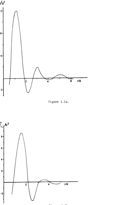
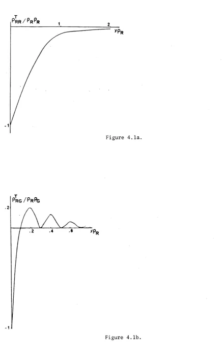
To gain some insight into why this is so, consider the short distance behaviour of the correlations as revealed by figure 1. Take special note of the maximum probability peaks at approximately
T T
a distance 1/Q in the p+^ plot 3/2Q in the p+^ +? plot T
and 2/Q in the p+9 + 9 plot, the exact location of the peaks being distances 6%, 3% and 2% greater respectively. Writing r ^ for the spacing between a particle of charge otq and a particle of charge 6q , we thus have as a good approximation at T = 1 ,
r u , r 12, r22 = Q'1 , 3Q_1/2, 2Q"1 (1.8.1)
which is the spacings predicted by local charge neutrality. Most
importantly, the short range behaviour of the correlations indicate there is little of no preferred sequential ordering of the +q and +2q
charges. The two species of charges have thus mixed.
The reason for the appearance of an oscillatory term can now be understood as a consequence of the mixing. At large distances a fixed test charge cannot distinguish a +2q charge from two +q charges at positions 1/2Q either side of the position of the +2q charge. The test charge thus "sees" the incipient crystalline structure of the corresponding one component system which has lattice spacing 1/Q .
Now consider the excess free energy of mixing. From table 1.1 we see f ex')
at T = 1 BAcf) is positive. We know from plots of the correlation f ex') functions that the two component plasma does mix, but in view of ßA^r being positive we might enquire into the thermodynamic reasons for this.
gas. We note, in view of the comment after (1.5.1), the relative volume occupied by charge species is determined by the charge density, which must be the same in all systems. Thus the +q charges must occupy a
portion x + 2x?) of the volume and +2q charges a portion
2x^/(x^ + 2x?) , so Acj)^^ is given by
A<£(id) (id) (a+b)N
2ttR - * (id)
r 2 x ? + x
p = --- aN
1
x iJ
2irR- 4>
(id) '2x2+x^ ' bN
2ttR (1.8.2)
Here the first term on the right denotes the free energy of a two
component ideal gas of aN particles of species 1 and bN particles of species 2 , the other terms on the right denoting the free energy of the one component ideal gas. Evaluating the right hand side of (1.8.2) we have
3A(t>( l d ) = -(log(2-x1)-(l-x1log2)
+ x 1logx1 + x 2 logx2 . (1.8.3)
Computation of (1.8.3) shows ßAcj)^^ to be negative and some thirty times the magnitude of ßAcf» 'J . Thus the total free energy of mixing
per particle is negative, so the system does mix.
From table 1 we see at T = 1 , 0 < ßA(j>^eX^ < 0.017 , which is
mixing of the ideal gas. Subtracting out this portion we need only
consider the free energy of any one of the ordered states. In particular we can consider the state in which the +q and +2q charges are
separate, occupying a portion x^/(x^ + 2x^) and 2x2/(x^+ 2X2), of
the volume respectively. Thus we would expect
«Kr.Q'.xp a A<f.( l d ) 4-
x^cr.Q'.x^i)
4 x2<Kr,Q',Xl=0) • (1.8.4)But A<|) is given by (1.8.2) so we can write (1.8.4) as
<t
>(ex’
1
(r,Q' , x p = x1
<(i( e x ) ( r , Q ' , x1
=i) + x2
<t>(ex5
(r,Q' , x1
=o) .(1.8.5)
Recalling the definition (1.5.2) this is equivalent to saying
3AcJ)^eX') = 0 (1.8.6)
which is in qualitative agreement with what we observe at T = 1. Equation (1.8.6) is well known from approximate studies of two component systems with a rigid neutralizing background in the case of the three dimensional Coulomb potential within a three dimensional domain
0.2 13.47025 -2.35813 0.00862 .37%
0.3 8.21473 -2.11494 0.01200 .57%
0.4 5.57299 -1.92080 0.01460 .76%
0.5 3.97258 -1.72572 0.01625 .94%
0.6 2.88719 -1.52947 0.01674 1.09%
0.7 2.08754 -1.33181 0.01581 1.19%
0.8 1 .45110 -1.13234 0.01308 1.15%
Table 1.1. Values of the quatities (1.4.1), (1.4.16), (1.5.5) and the percentage P = | (3A4^eX^/f(1,x^) | x 100%,
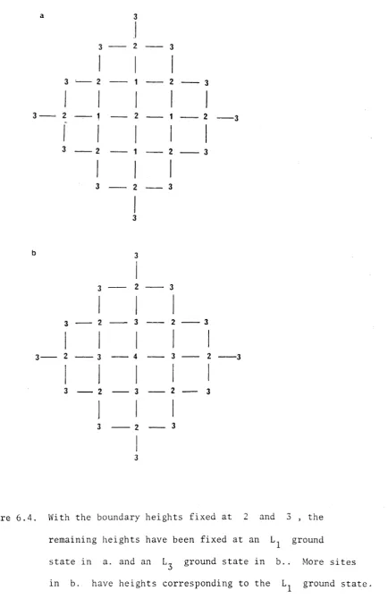
[image:39.564.62.501.144.759.2]Figure 1.1a.
[image:40.564.45.512.47.751.2]CHAPTER 2: EQUILIBRIUM POSITIONS OF THE TWO-COMPONENT PLASMA
2.1 Stieltjes, electrostatics and the zeros of the classical polynomials We now study the equilibrium position of the charges in a
two-component system. Polynomial identities in the form of determinants played an essential role in the calculations described in chapter 1. Here again polynomials and polynomial identities are the necessary mathematical tools.
Problems of the type to be discussed in this chapter were first considered almost a century ago by Stieltjes (1885a., 1885b., 1886)
(see also Szegö 1959 , chapter 6). Indeed we use Stieltjes'technique of writing the equilibrium positions of the charges as the zeros of a polynomial, and then determining the differential equation satisfied by the polynomial (and thus the polynomial) via the non-linear equations specifying the minimum. In Stieltjes1 work the polynomials that occured were the classical polynomials. Similarly, the solution of all the electrostatics problems considered here can be written in terms of the zeros of the classical polynomials.
Properties of the ground states can be described in detail, as the zeros of the classical polynomials have been extensively studied. Conversely, many intuitively obvious properties of the electrostatics problems can be formulated as theorems regarding the zeros of the classical polynomials, thus providing electrostatic interpretations to those theorems.
2.2 Two impurities on the circle
potential (1.1.3). At 0 = 0 fix a particle of charge +q and at 0 = tt fix a particle of charge +p . The uniform neutralizing
background necessary to obtain thermodynamic stability is not relevant when calculating the ground state equilibrium positions since it only contributes a constant to the Hamiltonian. Thus ignoring constant terms we may take for the Hamiltonian
2N i0 2N i0
Hn =
-q
l
l°g 11 -e |-pI
log!1+e Ik=l k=l
i0k i0.
I
losle -e 3 | . (2.2.1)l < k < j < 2 N
Note that the radius has been scaled out of the Hamiltonian. We seek the minimum of H^ subject to the requirement
0 < 0j < tt j = l,2,...,N and tt < 0^ < 2tt j = N+l,...,2N (2.2.2)
Further, without loss of generality we can choose for each j
6j < 6j+ l • (2.2.3)
Since H^ is real, continuous and bound from below such a minimum exists. The minimum is also unique. This follows from the
inequality
(A+B)
J-sin — 2— ^ (sinA sinB) 2 , 0 < A , B . < tt , (2.2.4)
minimum. The location of the minimum is given by the following result.
Theorem 2.2.1
The minimum of the function Hq subject to the constraint
(2.2.2) occurs at the zeros of the Jacobi polynomial l/~> P 1/2) (c o s q) ^ 0 < 0 < 2tt .
Proof
Using the identity
i s . ie _ ie. ie
Ie J-e I = i" (e 3-e K)exp - -j(6j + \ ) , 0j > ek (2.2.5)
we see the condition for a minimum is the set of non-linear equations
„ i0v i0v i0v i0v
0 = ^ - 0 = -i(qe /(e -1) + pe /(e K+l) - (2N-l+p+q)/2 JÖk
2N i0,
ie,
ie.+ V e /(e K-e :)) , 1 < k < 2N , j=l
(2.2.6)
where the prime on the sum indicates the j = k term is to be omitted. Following Stieltjes consider the polynomial
2N ie
f(x) =
n
(x-e *) 1=1(2.2.7)
which has its zeros at the minimum of . A short calculation then shows
i0k i0v N , i0v i0
-f"(e )/f'(e K) = 2 I 1/(e k -e J) j = l
Thus we can write the ground state condition (2.2.6) as
i0k 2i0 i0
0 - e K (e -l)f"(e )
i0k i0k i0k i0k 2i0, i0,
+ (2qe (e +1) + 2pe (e -1) - (2N-l+p+q)(e -l))f'(e J
1 < k < 2N (2.2.9)
The (2N+l)th order polynomial
x(x -l)f"(x) + (2qx(x+l)+2px(x-l)-(2N-l+p+q) (x2- l ) ) f (x) (2.2.10)
i0k
therefore has zeros at x = e , k = 1,2,...,2N and so is proportional to (x-A)f(x) where A is a constant. By equating like powers of
2N+1
x we find the proportionality constant to be 2N(p+q) so
x(x2-l)f"(x) + (2qx(x+l)+2px(x-l) - (2N-l+p+q)(x2-l))f ’(x)
- 2N (p+q)(x-A)f(x) = 0 (2.2.11)
It follows from the uniqueness of a minimum of that there is one and only one value of A such that (2.2.7) satisfies (2.2.11) with the 0^ constrained by (2.2.2). When N = 1 it is a simple exercise to derive
We now verify the choice (2.2.12) gives the required polynomial
solution of (2.2.11) for general N . By making standard transformations
applicable to second order differential equations (Szegö 1959, p. 16)
i 0
and then changing variables x = e we write (2.2.11) with A given
by (2.2.12) in the form
u" + (q(l-q)/(4sin“ 0/2) + p (1-p)/ (4cos2 0/2) + (2N+p+q)2/4)u = 0
(2.2.13)
where
u(0) (sin^0/2)(cos^0/2)
-iN0
e f (eiO
)
(2.2.14)However (2.2.13) is also a transformed version of the differential
equation of the Jacobi polynomials (Szegö 1959, p. 67) and satisfied by
u(0) = (sinq9/2) (cosP 0/2)P1fq‘1/2’p‘1/2:) (COS0) . (2.2.153
Hence we have
iO f(e )
iN0
e (q-1/2,p-1/2)
N (COS0) (2.2.16)
which is the desired polynomial solution of (2.2.11) satisfying the
constraint (2.2.2).
Theorem 2.2.1 is to be compared to Stieltjes interpretation
(Szegö 1959, p. 140)
Theorem 2.2.2 (Stieltjes)
T
I
(log (1+ x, )P + log(l-xk)Q) -l
log|x ,-x.k=l 1 < k < j < N K
3
P , Q > 0 , -1 < x^ < 1 , occurs at the zeros of the Jacobi polynomial
P^2Q-1’2P-1)
(X) .The expression T is the Hamiltonian for N unit charges confined to the interval [-1,1] by a particle of charge P fixed at x = 1 , and a particle of charge Q fixed at x = -1 , interacting via the
logarithmic potential. Thus comparing theorems 2.2.1 and 2.2.2 we see the equilibrium positions are closely related. Consider the unit circle in the complex plane. At z = 1 fix a particle of charge q = 2Q - 1/2 and at z = -1 a particle of charge p = 2P - 1/2 (p,q ^ 0) . If the equilibrium positions of the 2N charges as given by theorem 2.2.1 are projected orthogonally onto the real axis, then we locate the equilibrium positions of Stieltjes problem, theorem 2.2.2.
2.3 The thermodynamic limit: unit charges about an impurity
Reconsider theorem 2.2.1. The positions of the unit charges around an impurity (the +q charge at 0 = 0 say) in the large N limit are of particular interest. We have the following theorem (Szegö 1959, p. 193)
Theorem 2.3.1
Let x^N > x?N > ... be the zeros of P^a ’^(x) in [-1, +1] in decreasing order (a,3 real but otherwise arbitrary). If we write x .. = COS0 .. , 0 < 0 < TT , then for fixed v
vN vN v n
lim N0
IM-*» VN jv,a
Regarding the N -* 00 limit as the thermodynamic limit, with particle density tt/N , we have from theorems 2.2.1 and 2.3.1 the following
result.
Theorem 2.3.2
Consider the real line with a particle of charge +q fixed at the origin, and particles of unit charge at unit density immersed in a uniform neutralizing background. In the thermodynamic limit the ground state positions of the unit charges are given by
± j „ , , J ^
v , q - l / 2 1,2,...
There are several intuitively obvious properties of the ground state of the impurity problem. Let us list three:
(i) The cases q = 0 and q = 1 give a one-component plasma. When q = 0 the unit charges will form a lattice at the odd half integers. When q = 1 the unit charges will form a lattice at the integers.
(ii) As q increases, the unit charges will repel away from the origin (iii) At large distances from the origin the only effect of the +q charge will be to shift the one component lattice a distance q/2 each side of the origin. Thus the system is asymptotically charge neutral. From theorem 2.3.2 these properties can be formulated as theorems regarding the zeros of the Bessel functions. We thus have respectively
(i) The zeros of J - ^ O Z ) occur at the odd half integers. The zeros of occur at the integers (excluding zero).
(ii) For each V = 1,2,... and a > -1/2
3 j v,a
a t t h e odd h a l f i n t e g e r s s h i f t e d by +q/2 on t h e p o s i t i v e r e a l a x i s
and by - q / 2 on t h e n e g a t i v e r e a l a x i s .
M a t h e m a t i c a l p r o o f s o f t h e s e s t a t e m e n t s can be f ound i n Watson
( 1 9 5 8 ) , p p . 5 4 , 508 and 509 r e s p e c t i v e l y .
C o n v e r s e l y , t h e known m a t h e m a t i c a l t h e o r e m s r e g a r d i n g t h e z e r o s
o f t h e B e s s e l f u n c t i o n s can be u s e d t o d e s c r i b e t h e p o s i t i o n s o f t h e
u n i t c h a r g e s a b ou t t h e i m p u r i t y . Let us d e n o t e t h e p o s i t i o n s o f t h e
u n i t c h a r g e s on t h e p o s i t i v e r e a l a x i s by x ^ x ^ , . . . . Then from Watson
(1958) p . 518 we have from t h e o r e m 2 . 3 . 2 t h e c o n v e x i t y i n e q u a l i t i e s
which q u a l i t a t i v e l y d e s c r i b e t h e gr oun d s t a t e .
2 . 4 A s i n g l e i m p u r i t y on t h e l i n e
In §2.2 i t was shown how an e q u i l i b r i u m p r o b le m on t h e c i r c l e gave
r i s e t o t h e J a c o b i p o l y n o m i a l s . In t h i s s e c t i o n we c o n s i d e r an a n a l o g o u s
p h y s i c a l p r o b l e m , i n wh ich t h e e q u i l i b r i u m p o s i t i o n o f t h e c h a r g e s ar e
g i v e n i n t e r m s o f t h e L a g u e r r e p o l y n o m i a l s .
C o n s i d e r 2N p a r t i c l e s o f u n i t c h a r g e f r e e t o move on t h e r e a l X. > x? - x 1 > . . . > x , - x > . . . > 1 , q > 1
n+1 n ( 2 . 3 . 1 )
x. < x0- x 1 < . . . < x ..-x < . . . < 1 , 0 < q < 1
1 2 1 n+1 n , n ( 2 . 3 . 2 )
l i n e w i t h a p a r t i c l e o f c h a r g e +q f i x e d a t t h e o r i g i n . The s yst em
i s made e l e c t r i c a l l y n e u t r a l by im po si n g a b a c k g r o u n d c h a r g e d e n s i t y
° ( y )
■ (c/tt) ( l - y 2/ L 2) 1/2 Iy I < L
o | y| > l , ( 2 . 4 . 1 )
c = 2 ( 2N +q ) /L .
To compute t h e H a m i l t o n i a n f o r t h e s ys te m we r e q u i r e t h e i n t e g r a l
(Mehta 1967, p . 44)
^ J
d y ( l - y 2/ L 2 ) 1/2 l o g I x - y | = x 2/2L + K ( 2 . 4 . 2 )" L
where K i s d e p e n d e n t o f x . T h i s g i v e s us t h e c o n t r i b u t i o n t o t h e
H a m i l t o n i a n o f t h e p a r t i c l e - b a c k g r o u n d i n t e r a c t i o n . Thus i g n o r i n g c o n s t a n t
t e r m s , t h e H a m i l t o n i a n i s g i v e n by
2N 2N
H = (c/2L) I x - q I l o g IX,
j = l J k=l K
I
1 < j < k < 2N ( 2 . 4 . 3 )
where we have l a b e l l e d t h e 2N u n i t c h a r g e s x^ , x 2 , . . . x ?^T .
We s eek t h e minimum o f H^ s u b j e c t t o t h e c o n d i t i o n N p a r t i c l e s
a r e e i t h e r s i d e o f t h e i m p u r i t y a t t h e o r i g i n , t h a t i s
xR < 0 k = 1 , 2 , . . . ,N and xR > 0 k = N + 1 , . . . , 2 N .
( 2 . 4 . 4 )
unique (as in §2.2 the function is concave; see also Szegö 1959, p.
140). By symmetry we must have
"xk = xN+k * k = • (2.4.5)
The location of the minimum is given by the following result.
Theorem 2.4.1
The minimum of the function subject to the constraint (2.4.5)
occurs when the are the zeros the Laguerre polynomial
I'N*” 1/2') (c x2/L) (2.4.6)
Proof
The condition for a minimum is the set of non-linear equations
3H 2N
0 = 3— — = (c/L)X, - y ’ — ---, k = 1,... ,2N . (2.4.7)
k j=l k j k
Consider the polynomial
2N
g(x) = TI (x-xj (2.4.8)
Z = l
which has its zeros at the minimum of . Then we can write (2.4.7) as
Thus we have a ( 2 N + l ) t h o r d e r p o l y n o m i a l which h a s t h e 2N z e r o s
o f g ( x ) . Hence
x g " ( x ) + ( - ( 2 c / L ) x + 2 q ) g ' ( x ) + a ( x - b ) g ( x ) = 0 ( 2 . 4 . 1 0 )
By e q u a t i n g l i k e c o e f f i c i e n t s o f x we f i n d a = 4Nc/L . F u r t h e r m o r e
t h e symmetry c o n d i t i o n ( 2 . 4 . 5 ) r e q u i r e s g t o be e v e n . U s i ng t h i s
c o n d i t i o n i n ( 2 . 4 . 1 0 ) g i v e s b = 0 .
1/2
R e p l a c i n g x by ( L x/ c ) t h e d i f f e r e n t i a l e q u a t i o n assumes
t h e form
xu" + ( - x + ( q + 1 / 2 ) ) u ' + Nu = 0 , ( 2 . 4 . 1 1 )
u ( x ) = g ( ( L x / c ) 1//2) ( 2 . 4 . 1 2 )
We r e c o g n i z e ( 2 . 4 . 1 1 ) as t h e d i f f e r e n t i a l e q u a t i o n s a t i s f i e d by t h e
L a g u e r r e p o l y n o m i a l (Szegö 1959, p . 100) so t h a t
u ( x ) = L ^ - 1/ 2) (x) ( 2 . 4 . 1 3 )
S u b s t i t u t i n g ( 2 . 4 . 1 3 ) i n ( 2 . 4 . 1 2 ) , t h e o re m 2 . 4 . 1 f o l l o w s i m m e d i a t e l y .
As L -* °° and y r e m a i n s f i n i t e a ( y ) -> -c/tt . T h e r e f o r e i n
2 t h e t hermodynami c l i m i t c h o o s i n g c = tt (and t h u s L = 2(2N+q)/iT )
t h e b a c k g r o u n d ar ou n d t h e o r i g i n t e n d s t o a c o n s t a n t u n i t d e n s i t y . From
t h e o r e m 2 . 3 . 2 we know t h e e q u i l i b r i u m p o s i t i o n o f u n i t c h a r g e s immersed
on t h e l i n e . Hence from t h e e q u i v a l e n c e o f t h e two p h y s i c a l p r o b le m s
i n t h e thermodynami c l i m i t we c a n deduce t h e w e l l known t h e o re m r e l a t i n g
t h e z e r o s ' o f t h e L a g u e r r e p o l y n o m i a l s t o t h e z e r o s o f t h e B e s s e l f u n c t i o n s
(S zeg ö 1959, p . 1 9 3 ) .
Theorem 2 . 4 . 2
Le t y 1N < y 2N < . . . be t h e z e r o s o f L^q_1^ 2 ') (y) i n i n c r e a s i n g
o r d e r . Then
lim Ny
N-x» 4 ^ £ , q - l / 2 ' )
2 . 5 C r y s t a l l a t t i c e s on t h e c i r c l e
In t h i s s e c t i o n c r y s t a l l a t t i c e s t r u c t u r e s a r e g i v e n f o r t h e
e q u i l i b r i u m p o s i t i o n s on t h e c i r c l e o f two component s y s t e m s . By a
c r y s t a l l a t t i c e we mean a l a t t i c e which h a s a c e l l r e p e a t e d p e r i o d i c a l l y .
We have t h e f o l l o w i n g r e s u l t .
Theorem 2 . 5 . 1
Suppose t h e r e a r e nM p a r t i c l e s o f u n i t c h a r g e and M p a r t i c l e s
o f c h a r g e +q on t h e c i r c l e w i t h one o f t h e +q c h a r g e s f i x e d a t 0 = 0 .
R e q u i r e t h a t b et wee n e v e r y two +q c h a r g e s t h e r e a r e n u n i t c h a r g e s .
Then t h e e q u i l i b r i u m p o s i t i o n o f t h e nM p a r t i c l e s o f u n i t c h a r g e a r e
g i v e n by t h e z e r o s o f
Pn / ? " 1 ') // 2, "1 / 2 ') ( cos M0) 0 < 0 < 2tt ( 2 . 5 . 1 )
P ( n - l ) / 2 2 , 1 / 2 ’) (cosM0)> 0 < 6 < 2tt ( 2 . 5 . 2 )
i f n i s od d. The e q u i l i b r i u m p o s i t i o n o f t h e (M-l) p a r t i c l e s o f
c h a r g e +q o c c u r a t
0 = 2rrk/M k = 1 , 2 , . . . , (M-l) . ( 2 . 5 . 3 )
P r o o f
Label t h e c o - o r d i n a t e s o f t h e p a r t i c l e s o f c h a r g e +q
^0 = 0 > $1 » • • • ,<J>m_i and t h e p a r t i c l e s o f u n i t c h a r g e , 0O, . . . , 0 .
Then t h e H a m i l t o n a i n f o r t h e s y s t e m i s
o i 0 - i<J>,
H2 = "^ I l o g I e 3- e k |
0 < j < k < M-l
-q
l
0 < j < M-l 1 < k < nM
i(J>. icf),
I l o g eI 3- e
i 0 . i 0
I I l o g e 3- e
1 < j < k < M
( 2 . 5 . 4 )
Again i t i s e a s y t o show t h e e x i s t e n c e and u n i q u e n e s s o f t h e r e q u i r e d
minimum (Szego 1959, p . 1 4 0 ) . To p r o v e t h e t h e o r e m we must show t h e
e q u a t i o n s f o r a minimum, o b t a i n e d by t a k i n g p a r t i a l d e r i v a t i v e s o f ,
a r e s a t i s f i e d when t h e a n g l e s a r e g i v e n by ( 2 . 5 . 1 ) , ( 2 . 5 . 2 ) and ( 2 . 5 . 3 ) .