Implementation of the Wavelet-Galerkin method for boundary value problems

Rochester Institute of Technology

RIT Scholar Works

Theses

Thesis/Dissertation Collections

1998

Implementation of the Wavelet-Galerkin method

for boundary value problems

Adam Scheider

Follow this and additional works at:

http://scholarworks.rit.edu/theses

This Thesis is brought to you for free and open access by the Thesis/Dissertation Collections at RIT Scholar Works. It has been accepted for inclusion

in Theses by an authorized administrator of RIT Scholar Works. For more information, please contact

[email protected]

.

Recommended Citation

Implementation of the Wavelet-Galerkin Method

for Boundary Value Problems

by

Adam K. Scheider

A Thesis Submitted In

Partial Fulfillment of the

Requirement for the

Master of Science

In

Mechanical Engineering

Approved

by:

Professor

_

Josef S. Torok

Thesis Advisor

Professor

_

H. Ghoneim

Professor

_

K. Kochersberger

Professor

_

Charles Haines

Department Head

DEPARTMENT OF MECHANICAL ENGINEERING

COLLEGE OF ENGINEERING

ROCHESTER INSTITUTE OF TECHNOLOGY

Implementation of the Wavelet-Galerkin Method

for Boundary Value Problems

I, Adam K. Scheider, hereby grant permission to the Wallace Library of the

Rochester Institute of Technology to reproduce my thesis in whole or in part.

Any reproduction will not be for commercial profit.

DEDICATION

I dedicate this thesis first

and

foremost

in

loving

memory

of

Scott Crouch

and

in

living

recognition of

Thomas Haralson. These

two

men

have

touched

my

life in

such a special

way

that

I know I

will never meet anyone else

like

them.

I

believe

you can

only

meet

very few

people so

very

special.

Without

them

I

would

not

have

grown

to

be

the

man

that

I

am

today. And

I

would

not

have

completed

my

college career at

RIT in

the

manner

in

which

I have if I had

not

worked so

hard

to

make

them

so proud.

My family

took

no

small part

in

this

act.

If I

could give

any

piece

of advice

to

any

person,

it

would

be

to

not

take

your

family

for

granted.

The

prayers of

family

and

friends have

not gone

unnoticed,

especially

those

of

Sr.

Grace,

Sr.

Anne,

and

Fr.

Gentile.

I hold

the

Domes

and

the

Denicks

in

a

distinguished

place as well.

Finally,

I

would

like to

acknowledge

Dr.

Torok

and

the

rest of

the

Mechanical

Engineering

faculty. Without

them,

this

would

not

have been

TABLE OF CONTENTS

Abstract

...

1.

Introduction

to

Wavelets

2.

Example

-

Haar

Approximation

Table

2.1,

Subspaces

of

Haar Approximation

3.

Daubechies Wavelets.

4.

Variational Formulation

5.

Approximation

Methods to the

Variational

Form

6.

Galerkin Method

7.

Wavelet

-

Galerkin Method

.

8.

Example

-

Analytical

.

9.

Example Wavelet

-Galerkin.

10. Example

Galerkin

-

Quadratic

11. Conclusions

....

Bibliography

....

Appendix

A (Matlab

Programs)

.

11

15

16

20

24

26

30

32

34

42

48

50

[image:5.556.59.483.66.482.2]

Abstract

The

objective of

this

work

is

to

develop

a systematic method of

implementing

the

Wavelet-Galerkin

method

for approximating

solutions of

differential

equations.

The

beginning

of

this

project

included

understanding

what

a wavelet

is,

and

then

becoming

familiar

with

some of

the

applications.

The

Wavelet-Galerkin

method,

as applied

in

this paper,

does

not

use a wavelet

at

all.

In

actuality,

it

uses

the

wavelet's

scaling function. The distinction between

the

two

will

be

given

in

the

following

sections of

this

paper.

The

sections of

this thesis

will

include

defining

wavelets

and

their

scaling

functions.

This

will give

the

reader

valued

insight

to

wavelets

and

Discrete

Wavelet Transforms (DWT).

Following

this

will

be

a section

defining

the

Galerkin

method.

The

purpose

of

this

section will

be

to

give

the

reader an

understanding

of

how

weighted

residual

methods

work,

in

particular, the

Galerkin

Method.

Next

will

be

a

section

on

how

Scaling

functions

will

be implemented in

the

Galerkin

method,

forming

the

Wavelet-Galerkin Method.

The focus

of

this

investigation

will

deal

with

solutions

to

a

basic

homogeneous differential

equation.

The

solution of

this

basic

equation will

be

analyzed

using

three separate,

distinct

methods,

and

then the

results will

be

compared.

These

methods

include

the

Wavelet-Galerkin

Method,

the

Galerkin

Method using

quadratic

shape

functions,

and standard analytical means.

Factors

to

be

studied

include

computational

time,

effort, accuracy,

and ease of

After

a

thorough

comparison

has been

made, there

will

be

a section

to talk

about possible applications of

the

Wavelet-Galerkin

method and

recommendations

for future

work.

Predictions

of

what avenues

to

pursue

in

refining

the

Wavelet-Galerkin

method will

also

be

stated.

And

suggestions

on

CHAPTER

1

Introduction

to

Wavelets

A

wave

is usually defined

as

disturbance in

time

or

space.

Periodic

waves,

such as a

sinusoid,

repeat after a

finite interval.

Fourier

analysis

is

wave

analysis.

It

expands signals or

functions in

terms

of

sinusoids

(or,

equivalents,

complex

exponentials)

which

has

proven

to

be extremely

valuable

in

mathematics, science,

and

engineering,

especially for

periodic,

time-invariant,

or

stationary

phenomena.

A

wavelet

is

a

"small

wave",

which

has its energy

concentrated

in

time

to

give

a

tool

for

analysis of

transient,

nonstationary,

or

time-varying

phenomena.

It

still

has

the

oscillating

wavelike characteristic

but

also

has the

ability

to

allow

simultaneous

time

and

frequency

analysis

with

a

flexible

mathematical

foundation.

This is illustrated

below

with

the

wave

(sinusoid)

oscillating

with

equal amplitude over

-oo<t<oo

and,

therefore,

having

infinite

energy

and with

the

wavelet

having

its

finite

energy

concentrated around a point or

instant

of

time.

(a)

A Sine Wave

(b)

Daubechies'

Wavelet

Voao

We

will

take the

wavelets and use

them

in

a series expansion of signals or

CHAPTER

1

represent a signal or

function. The

signals are

functions

of a

continuous

variable,

which

often represents

time

or

distance.

A

signal or

function

can often

be better

analyzed or

described

or

processed

by

decomposing

it into

a series or summation.

An

example

of

this

would

be digital

signal

processing (dsp).

Say

whatever

object

that

is

supposed

to

pick

up

the signal,

a

microphone, accelerometer,

guitar

pickup,

etc...

is too

sensitive

and

the

signal

has

a

significant

amount of static or

interference.

By

expressing

the

signal

a

summation of

terms,

it

would

be

possible

to throw

out

the

terms that

are

causing

the

unwanted

noise,

leaving

only

the

clear

portion of

the

signal.

Therefore,

the

first

step is

to

express

the

signal as a

series expressed

by

linear decomposition

by

/(/>=

2X^(0

(1.1)

k

where

k

is

an

integer

index for

the

finite

or

infinite

sum.

The

coefficients

ai<

are

real-valued expansion coefficients and

Tk(t)

are a

set

of

real-valued

functions

of

t

called

the

expansion

set.

If the

expansion set

is

unique,

it is

called a

basis.

A

basis

is

orthogonal

if its inner

product

of

distinct

basis functions is zero, that

is

(%(t)X(t))

=

\X(0%

(t)dt

=

0

h*l

If

the

basis is

orthogonal, then the

coefficients

in

(1.1)

may be

calculated

by

multiplying both

sides

by

the

generic

function

TkO)

and

taking

the

inner

product:

ak=(f(t),%(t))

=

\f(tm(k)dt

CHAPTER

1

For

a

Fourier

series, the

orthogonal

basis functions

are

sin(kQ0t)

and

cos(kcoot)

with

frequencies

of

kco0.

For

a

Taylor's

series, the

nonorthogonal

basis

functions

are simple monomials

tk,

and

for many

other

expansions

they

are

various polynomials.

There

are expansions

that

use splines

and

even

fractals.

For

the

wavelet

expansion,

a

two

parameter system

is

constructed such

that the

linear decomposition is

of

the

form

/(0

=

IZA(o

(1.3)

k 1

where

bothy

and

k

are

integer indices

and

the

^(t)

are

the

wavelet expansion

functions

that

usually form

an orthogonal

basis.

The

set

of expansion

coefficients

ajik

are called

the

discrete

wavelet

transform

(DWT)

of

f(t)

and

the

linear decomposition

expression

is

the

inverse transform.

Wavelet Systems

Wavelet

expansions are

not

unique.

That

is,

there

may be

more

than

one

wavelet system

that

may successfully

represent

a signal or

function.

However,

all

of

them

seem

to

have

three

basic

characteristics:

1

.

A

wavelet system

is

a

set

of

building

blocks

to

construct or represent

a

signal

or

function.

It is

a

two-dimensional

expansion

set

(

usually

a

basis,

which

means

it is unique) for

some

class

of

one-

(or

higher)

dimensional

signals.

In

other

words,

if

the

wavelet

set

is

given

by

^(tjfor indices

of

j,k

=

CHAPTER

I

for

some set of coefficients aj,k.

2.

The

wavelet expansion gives a

time-frequency

localization

of

the

signal.

This

means most of

the

energy

of

the

signal

is

well-represented

by

the

discrete

expansion

coefficients,

a-^.

3.

The

calculation of coefficients

from

the

signal

may be done

efficiently.

Many

wavelet

transforms

may

be

calculated

with

O(N)

number

of

operations.

This

means

the

number

of

floating-point

multiplications

and

additions

increase

linearly

with

the

length

of

the

signal.

More

general wavelet

transforms

require

0(Nlog(N))

operations,

essentially

the

same as

the

Fast Fourier Transform (FFT).

A

Fourier

series maps

a one-dimensional

function

of a continuous

variable

into

a

one-dimensional sequence

of

coefficients.

Whereas

the

wavelet

expansion

maps

it into

a

two-dimensional

representation

that

allows

localizing

the

signal

in

both

time

and

frequency. A

wavelet

representation will

give

location in both

time

and

frequency

simultaneously.

By

this explanation,

a

wavelet

representation

resembles

a

musical score

in

a

way,

where

the

location

of

the

notes

tells

when

the tones

occur and

what

their

frequencies

are.

There

are

three

more

additional

characteristics,

which

are more specific

to

wavelet expansions.

These

are not

so much

characteristics

but

properties

that

CHAPTER

I

1

.

All

first-generation

wavelet systems are

generated

from

a

single

scaling

function

or

wavelet

by

simple

scaling

and

translation.

The

two-dimensional

parameterization

is

attained

from

the function

Tj,k(t)=2j/2vF(2jt-k)

where

j

and

k

are elements of

Z,

the

set

of

all

integers.

This

equation

is

sometimes

referred

to

as

the

"mother

wavelet".

The factor

2j/2

maintains

a

constant

norm

independent

scale

of

j.

This

parameterization

of

the time

or

space

location

by

k

and

the

frequency

or

scale

by j (really

the

log

of

the

scale)

is

extremely

effective.

2.

In addition,

almost

all

useful

wavelet

systems

satisfy

multiresolution

conditions.

This

means

that

if

a set of

signals

can

be

represented

by

a

weighted

sum of

cb(t-k),

then

a

larger

set

(which includes

the

original)

can

be

represented

by

a

weighted

sum

of

<j>(2t-k).

Basically,

if

the

basic

expansion

signals are made

half

as

wide

and

translated

in

steps

half

as

wide,

they

will

represent a

larger

class of

signals

exactly

or give

a

better

approximation of

any

signal.

This

last

statement

is in

essence

what makes wavelets work!

3.

Lower

resolution

coefficients

may

be

calculated

from higher

resolution

coefficients

(via

a

filter bank).

This

allows a

very

efficient calculation of

the

expansion

coefficients

and

relates wavelet

transforms to

a

known

CHAPTER

1

Multiresolution

formulation

requires

two

closely

related

functions,

which

are

the

wavelet

*P(t)

and

the

scaling

function

<f>(t).

Together,

these

functions

allow a

large

class of

functions

to

be

expressed

by

the

form

f(t)

=

Z

cJ(<-*)+

Z

Y,d.kV(2>t-k)

(1.4)

<T=-C0 *T=-00 j=Q

Another form

of

this

equation

is

given

below.

It is

created

by

substituting

the

mother wavelet expression

into

the

above

equation.

g(t)

=

ZS0

(k)2i0,2^(2Ju-k)

+

YdJ:dj(k)2^^(21t-k)

(1.5)

k k

j=j0

A very

interesting

fact

should

be

noted

here,

before

we

go

any farther.

Each

j

term

of

the

summation represents

its

own

subspace

of

the

approximation.

The

terms

^(t)

actually

span

the

differences between

the

approximations spanned

by

the

various scales of

the

scaling function.

To

describe this

better,

a more general view should

be

taken.

The

goal

of

the discrete

wavelet

transform

(DWT),

eqn

(1

.5),

is

to

approximate a

function

or

signal

over

an

interval

in L2(R). This is

the

space of

functions

f(t)

with a

well

defined integral

of

the

square

of

the

modulus of

the

function.

L2(R)

is

also

known

as

the

space

of

finite-energy

signals.

The

"L"

signifies a

Lebesque

integral,

the

"2"

denotes the integral

of

the

square of

the

modulus of

the

function,

and

R

states

that the independent

variable

of

integration t is

a number over

the

whole real

line.

For

a

function

g(t)

to be

a member of

that space,

it is denoted by: g

e

L2(R)

or

simply

g

e

L2

Although

most

of

the

definitions

and

derivations

are

in terms

of

CHAPTER

1

example,

polynomials

are

not

in

L2,

but

can

be

expanded over

any

finite domain

by

most wavelet systems.

Anyway,

if

the

j's

reached

to

infinity,

the

approximation would

span all of

L2

Since

all of

the

j's

represent

the

difference between

the subspaces, the

symbolic representation

would

look like

this:

L2

=VQW0W,W2...

It is important

to

note

that the

scale of

the

initial

space

is

arbitrary

and could

be

chosen at a

higher,

or

lower,

resolution.

That is to

say

that

jo

could

take

on

any

positive

or negative

integer

value we want

to

assign

it.

This

also

includes

negative

infinity.

Let's

take

a closer

look

at equation

(1

.5),

the

DWT formula. The first

summation, the

single

summation,

represents

only

one subspace.

It only

represents

one

term.

It is

the

initial

subspace.

The

value

of

c(k)

is

found,

almost

instinctually,

by finding

the

dot

product of

the

basic scaling function

{t)

and

the

function

we wish

to

approximate

g(t).

c(k)

=

c0(k)

=

(g(t)Mt))

=

\g{tyt>k(t)dt

(1

.6)

The

dj(k)

coefficients

are

found in

a similar

way

by dotting

the

function g(t)

with

the

wavelet

Tj,k(t),

not

the

scaling function

<f>(t).

d}(k)

=

d(j,k)

=

teCO^O)

=

\g(tyJk(t)dt

(1

.7)

The

coefficient

d(j,k)

is

sometimes

written as

dj(k)

to

emphasize

the

difference

CHAPTER

I

c(k)

is

also sometimes written as

q(k)

or

c(j,k)

if

a

more general

"starting

scale"

other

than

j=0 is

used

for

the

lower limit.

These formulas may

be

used

so

long

as

the

wavelet system

being

used

is

orthogonal.

This is

no minor

point

to

overlook.

Although,

most wavelet systems are orthogonal

in

nature.

This is

one

of

the

mathematical requirements

that

the

wavelets are

subjected

to

when

being

constructed.

We

shall now

define

the

scaling function

<(>(t)

and

the

wavelet

^(t).

Both

of

these

functions

are

based

upon recursion.

I

will

simply

state

the

definitions.

^(0

=

Z/2(")^(2^-)

neZ

(1.8)

n

T(0

=

][>i(")V2<zK2/-h)

neZ

(1.9)

n

In

these equations,

Z is

the

set

of all

integers. The

coefficients

h(n)

are

a

sequence

of real

or

perhaps complex numbers

called

scaling functions

and

the

V2

maintains

the

norm of

the

scaling function

with

the

scale

of

two.

The

coefficients

h^n)

are related

to the

scaling function

coefficients.

Due

to the

requirement

that the

wavelets

span

the

"difference"

between

the

subspaces and

the

orthogonality

prerequisite,

hi(n)

is

related

to

h(n) by

hi(n)

=

(-1)nh(1-n).

I

will

demonstrate how to

perform a

discrete

wavelet

transform

on a simple

CHAPTER

2

Example

-Haar Approximation

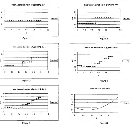
This

example

demonstrates how

to

use

a

discrete

wavelet

transform

(DWT)

to

approximate a given

function. The

function,

chosen

at

random,

is

defined

as

g(t)

= 5t2-

3t

+

1

.

The

wavelet

to

be

used

is the

simplest

wavelet

known.

It is

called

the

Haar

wavelet.

The Haar scaling function is

what

is

commonly known

as

the

unit

step function.

However,

if

the

formula

that is

given

for

the

scaling function

is

referred

to,

the

scaling function

has

coefficients

/2(0)

=

1/V2

and

/z(1)

=

1/V2.

>

t

Haar

Scaling

Function

<|>(t)

"?

t

Haar Wavelet

T(t)

The

initial scale,

j0,

was

chosen

to

be

zero.

As

stated

in

the

earlier

section,

it

could

be

chosen at random.

Zero

was

picked

because it

seemed

logical.

Also,

the

interval

on which

we want

the

approximation was picked

to

be

from

zero

to

one

because

it

seemed

logical.

The first step

was

to integrate the

function

times the

scaling function

over

the

internal. The scaling function is simply

the

unit

step function

from

zero

to

one.

c(k)

=

$

(5t

2

-3r

+

1)(1)a&

=

1

.

1 66667

CHAPTER

2

This

becomes

our

V0

subspace.

The

plot

is

shown on

the

following

page.

The

next subspace

is

approximated

by finding

d0(0). This

means

finding

the

value

of

the

integral

of

the

wavelet

times the test

function

over

the

interval.

05

d0(0)=

J(5f2

-3f

+

1)(1)df+

j(5t2

-3t

+

1)(-1)df

= -0.500000

05

This

spans

the

subspace

W0

which

is

the

difference between

the

adjacent

subspaces.

If

the

spreadsheet

is

referred

to,

look

at

the

W0

column.

It

shows

a

negative

0.5

value

halfway down,

and

then

a

positive

0.5 the

rest of

the

way.

This is due

to the

DWT formula. The

coefficient must

be

multiplied

by

its

wavelet.

In

this case, the

wavelet

simply

flops

from

positive

one, to

negative one.

The

next

step is

finding di(0)

and

di(1 ).

This

is

what

the

associated

wavelets

look like.

*i

0.5

0.5

These

graphs

show

how

the

scaling

and

translation

principles work.

The

wavelets

still

have the

same

height,

only

they

are

in different

places and scaled.

Both

of

these

wavelets

have

magnitudes

of

1

everywhere.

The

coefficients are

calculated

using the

following

formulas.

025 0.5

d,(0)

=

J(5f2-3f

+

1)(1)rf/

+

J(5r2

-

3/

+

1)(-1)df

=

0.031 2500

CHAPTER

2

075

d,

(1)

=

|(5r2

-3t

+

1)(1)<#

+

J(5r2

-3/

+

1)(-1)dSf

=-0.281

2500

0.5 0.75

These

coefficients

may

then

be

used

to

calculate

the

values

in

column

W1

.

They

must

be

multiplied

by

V2

and

by

the wavelet,

of course.

This

can

be

found in the

formula. The

approximation

to

g(t) may

be

found

by

summing

all

the

previous

subspaces,

including

V0.

At any

rate,

it

should

be

clear now

how

each

successive subspace

is

approximated.

The

graphs show a

few

more approximations.

It

can

be

seen

that

the

last

approximation

is

not a

very

good one.

However,

it does

serve

the

purpose

to

demonstrate how

the

DWT

works.

Also,

this

example

clearly

shows

how

coarse

the

Haar

wavelet

really is. The

challenge

is

to

find

smoother

wavelets

which are

still

orthogonal.

Ingrid Daubechies has done

a

lot

of work

in

this

area.

She

really

is

considered

to

be

one of

the

leaders in

wavelet

technology.

Haar Approximationof g(t)=5tA2-3t+1 Haar Approximationof g(t)=5tA2-3t+1 3 2 5 2

I

15 0 5 0

0 2 0 4 06 0.8 1

t

Figure

1 3 25 2 15 n 05 0

0 2 0 4 0.6 0

Figure 2

Haar Approximationofg(t)=5tA2-3t+1

02 04 06 08

[image:19.556.48.267.58.487.2] [image:19.556.59.513.59.488.2] [image:19.556.292.517.61.489.2]

Haar Approximationofg(t)=5tA2-3t+1 25 2 - 15-i -05

|-*-W2J

0 02 04 06 08 1 12

Figure 3 Figure 4

Haar Approximationof g(t)=5tA2-3t+1

r** r*^

|--W3|

cn

}

! C 02 04 06 08 1 1

t 2 35 -3 -2.5 -2 -1.5 -1 05 0J

Known Test Function

/

/

/

' known!'

^-^

~^~-~^^__

___

) 0.2 0.4 0 6 08

t

|

,_ ,_

m in ,_ T ^_ ^_

in in ^_ T_ ^_ T_

in in T_ ^_ .^ ,_

in m ,- ,-c CO CO CM CM 00 00 m in 00 00 CM CM CO CO CO CO CM CM 00 00 in in 00 00 CM CM CO CO

5

o

o o T T

CN CN CM CM Is- Is- in in in in m in r- r- CM CM CM CM ^~

T-o o

T CN CN CO CO CO CO CO CO o o oo 00 sr sr r~- r^- sr sr CO 00 o o CO CD CO CO CO CO CM

>!

m CO CO o o ^

T-in in in m r^ r^ _{sr sr}

d d

CD CD r-- r-~ _{o o} in in CO CD o o CO oo .* 00 00

r- Is- co co _o

o in in m m CO co CO CO o

q

CO CO ^ 00 00 CM CM in in O

d d d d d

d d d d d d

d d

T T

CN CM C\i CM

in in CO CO in ID CM CN oo 00 sr sr CD CD CO CO CD CD CN CM CD CD _CM

in o in CO CM in o in CO Is-CM Is-CD CD CO r-- Is-CN r--co CD CO CD CD CO CO m in in m CO CO CN CN CD CD sr sr sr sr r-- r~- CO CO in m T T

sr sr CD CD

CD CO o o CD CD Is- Is- CD CD o o CM CM h- r^- ^ ^ o O 00 oo r-- r-- CD CD T T

00 00 00 00 CM cm CO CO CO CO co CO 00 00 t

sr sr CD CD CO CO sr sr CM CM CD CO CO OO o o o o sr sr in in T ^ ^ o o m in m m CD CD CD CD o O CO CO CD Is- Is- CO CO co co Is- r- CD CO

5

t h- r^ CO CO CO CO r^ r- CM CM T T _{in in}

T T

CD CD 00 00 CO CO Is- Is- _{o o o O} T T

00 CO CD CD CN CN CO CO 00 00

5

CD

5

CD

sj--sr CD CD CO CO CO CO sr sr CD CD o o CO CO CD CD CO CO CD CD CO CO T ^ CM CM t ^~

Is- r- Is- Is- _{co CO CD CO} in m CO CD CO CD CD CO t T- T~ T

^j ^_; sr sr 00 00 CO CO o o

d d d d d d d d d d d d d d

^ ^ ^ ^ T '- *~ ^ *

T~

CM CM CM CM

.,- ,_

CD CD ,-

,-T T~ Is- Is- OO 00 in in r~-

r-CO CO r-- c- T ^_ _{CO CD}

CD CD in m CD CO in in CD CD _{CN CM} T~ x

CD co o o CO CD r^ t-~ sr sr TT sr CM CM T T _{o O} r~- t-- 00 00 sr sr CO CD CN CN o o CO CD CD CD o o r- r^ _{CN CM} sr sr CO CO T T

co co r

r--sr sr sr ^r O O sr sr CD CD CN CN 00 CO ^

T-CD CD T- ^^ _{o O CM} CM T CO CO CM CM CO CO CO CO sr sr CO sT f CN CN CN CN sr sf CO CO 00 00 CD CD o o o o 00 OO T~

T-CD co CM CM sr sr CO CO

5

CN CN CD CO sT sr CN CN CO CO in in t T

CD CD o o CN CM 00 00 CO CO CD CD o o sr sr CD CO CN CN CN CM T

o o T

T-T in in _{CM CM} CD CD sr sr CM CN in in CD co Is- r- o o CN CM o O T T

O o o o o o o o ^ T _{O O} CN CM o o sr sr o o in in _o o Is-

Is-O O

d d

o o

d d d d

o o

d d

o o

d d

o o

d d

o CD

d d q q d d

o o

c O

d

1 1

d d

1 i

d d

i

d d

1 1

d d

i i

d

d

i

d d

i 1

d d

o

CO 00 00 00 CO CO CO CO in in in in r~- r-- r- r-- CN CM CM CM r- r- Is- Is- CM CM CN CM

To

sT sr sT sr Is- Is- Is- Is- CO CO CO CO CD in sr CD CD in ^r CD CD in sr CO CD m sr co

m m m m 00 00 CO 00 CM CN CN CN O O o o

E

in m m m T T

^ ^ o o o o CO CO CO CO sr sr sr sr t- Is- r- r- t t ^ t

CD in in in in CD CD CD CD CD CD CD CD r- r~~ r- r- o o o o sr sr sr sr ^r sr ^ sr X CD CD CO CD in in in in CD CD CD CD co CD co CD h- r- r~- r- _{00 CO} oo 00 sr sr sr -sr

2

Is- r~- Is- r^ _{co co CO co} in in m in CO 00 00 CO 00 00 CO

cq

CM CM CM CM

Q.

d d d d d d d d d d d d d d d d

CM CM CM CM

<

_{m m m m}

00 00 00 OO 00 OO CO 00 in m m m CO CO CO CO m in m in OO 00 00 00 in in in in CO

CO

X

Is- Is- Is- Is- _{00 00 00 00 CO CO CO CO} r- r~- h- r^

CD CD CD CD CM CM CM CM 00 00 oo 00 Is- Is- Is- Is-00 oo 00 00 _{co co co co} sr sr sr sr co co CO CO in in in in CD CD CD CD co co CD CO 00 00 00 00 CN CD CD CD CD *r sr sr sr CO CO CO CO sr sr sr

"a-in in in in CD CD CD CD CD CO CO CD

^

sT sr sr

si-in in in in CN CM CM CN CO CO CO CO _{o o o o} T- T T-

T-r- Is- r-- Is- CD CD CD CD

*? ^ m in in in o o o o o O O o CN CM CM CN T T _{o o o o} Is- Is- h-

Is-o o o o o

d d d d d d d d

o o o O

d d d d

T_ T- T_ T_

d d d d

"-;

,_

^ ^

If)

CD

d

d d d

i 1 1 i

d d

d d

i i i o

d

o o 1 1 o o o o O

CO CM CN CN CN CN CM CM CM CD CD CD CD CD O) CD CD sr sr sr sr sr sr sr -sr Q_ CD CD CD CO co CD co CO Is- Is- Is- I-- r^- r~- r-- r^- ^ ^ ^ ^ ^ T*~ T~* ^ t T~" T T

V T T~" T"~

in CO OO 00 00 00 00 00 00 sr sr sr sr sr sr sr sr CD CD CD CD CD CD CD CD sr sr sr sr sr sr sr sr .0 CT)o o o o o o o o CN CN CM CM CM CM CM CN CO 00 00 00 00 OO 00 00 sr sr sr sr sr sr ^r -sr

3 t

^ ^ ^ T ^ t

V-CM CM CN CM CM CM CM CM CO CD CD CO CD CO CD CO CD CO CD CD co CD co co

CO Is- r- Is- Is- r- Is- r- r- CO CD co CD co CD CD CO CM CM CM CM CM CM CM CN o o O o o o o o

d d d d d d d d d d d d d d d d

CM CM CN CN cn CM CM CN

CM

*T Tf

Tj-sr sr sr sr sr sr sr sr sr sr sr "J"

sr 00 00 00 00 00 00 00 00 CO 00 00 00 00 00 CO 00 CD CD CD CD CD CD CD CD CD CD CD CD CD CD CD CD CD sr sr sr sr t sr sr sr sr sr sr sr sr sr sr -sr

25

i

TT ^r -3

TJ-sr sr sr

5 5 ^

sr

5

5 5 5

r~- r- r~- r-Is- r~- r-r~- Is-Is- Is-n. Is-Is- Is-r- Is-CO r- "ST o sr o sr o sT O sr o sr o sr o sr o sr o sr o sr o sr o sr o sr o sr o sr o CO CD CO CD CO CD CO CD CO CD CO CD CO CD CO CDCO

CD CO CD CO CD CO CD CO CD CO CD CD CO CO

d d d d d d d d d

i

d

d d d

i

d d d d

i

d d d

1

d

i

d d

1

d

1

d d d d d d d d

Is- Is- Is- Is- Is- Is- Is- Is- r Is- r-- r-- r^ r~- r^ r^ r^. r- r- r^ r- r-- r- r- r- Is- Is- Is- Is- Is- Is- r--CO CD co CO CD CD CO CD CD CO CD co CO co CD CD CD CD CD CD CO co CD CD CD CO CD co CD CD co co CD CO CD CO CO CO co CD CO CD CD CD CO CD CD CO CD CO CD co CD CD co CD CD co co CD co CD co co O) CD co CO co CO CD CD co CD CD CD CO co co CO CO co CO co co CD CD CO CO co CD co co CD CD co co CD CD CO co CO CD CO co CD CD CD CO CO CO CO CD CO CD co co CD co CD CO co CD CO CO CD CD CO CO CO CD co co CD CO co CD CD CD CO co co co CO CD CD CD co CO CD CD co co CD

cq

co

cq

co CO CO CO ci

d d d d d d d d d d d d d d d

o in in in in m in in in in in in in m in in in in in in in in in in m in in in U^ in m in in

5

o

i

d

i

d d

i

d

i

d d

i

d

d d

i

d

i

d d

i

d

i

d

i

d

i

d d d d d d d d d d d d d d d d

Is- t^ r- r- r-- r- r Is- Is- Is- r- h- r-~ r^ r~- r- t- r-^ r^ r^ r~- r r- r- r- Is- Is- Is- Is- Is- Is- Is-co co co CD co co co CO co CD co co co CO CD co CD CD CD co co co co co co co co CD co co co CO CD co CD co CD CO CD CD CO co CO CD CD CD CD CD CD CD CD CO co CD CD CD CD CD CO co co CO co co CO co CD co CD CD CO CD CO CO CO co CO CD co CD CO co co co co co CD CD CO co CD CD co co CO CO o _{co co co co CD CD CD CO} CO co CO CO co CO co CO co CO CD CD CO co co CO co CO CD CD co CD co co

>

co co co CD CO CD CD CO co CO CO CO CO CO CD CD CD CO CD CD CD CD co CO CO CO CO CD CD CD CD CO CO CO CO co co co CO CD co CO co co co CO co CO co CO CO CO CD CO co co co co CD co CD CD co co

-* _o in CN CD O in CN CO o in CM m CN in Is-00 in r-co in CM

d

in CN

d

in CM CO in CM CO in r-CO in CO in CO sr in CO sr in

d

in

d

in CM co in in CM co in m CM CO in CM co in r~-00 co in 00 CO in

r--d

in

d

m CM 00 tfj CN 00 in t-CD m Is-00 in r--co CD m Is-CD

d d d

d d d

d d d d d d

d d d d d d

d d d d d d

CHAPTER

3

Daubechies Wavelets

The

family

of

compactly

supported

wavelets

constructed

by

Daubechies in

1988

opened

the

door

to

a

whole new

territory

in

mathematics.

Compactly

supported means

being

defined

over a

finite,

usually small, domain.

In

fact,

the

impact

of

her

work

is

so powerful

that the

Wavelet-Galerkin

method should

be

renamed

the

Daubechies-Galerkin

method.

The

fundamental

aspect

is

that the Daubechies

set of

wavelets provide

an

orthogonal

basis

with which

to

approximate

functions.

As

with

all

wavelets,

the

basic recursion,

or

dyadic,

or multi-resolutional equation

takes the form

q>{x)^ak(p(2x-k).

(3.1)

k

The

ak's

are

a

collection of

coefficients

that

categorize

the

specific

wavelet

basis.

The

mother wavelet also

takes the

conventional

form

^(x)

=

(-1)V^(2*-*)

(3.2)

k

These formulas

are

standard

for

all

the

wavelets encountered

in

practice.

Daubechies

work

begins

when

she

sets

the

rules

on

how

to

define the

coefficients

ak.

First,

the

scaling

function

must

be

normalized

so

that

j<pdx

=

1

.

This

provides

for

the

normalization condition.

Nfak=2

(3.3)

k=0

Hence,

we refer

to

<p(x)

and

y/{x)

of

this

form

as a multiplier

2

system.

This

also

is

gives

the

2j/2

CHAPTER

3

one

can generalize

wavelet systems

to

any arbitrary

nonnegative

integer.

The

translates

of

<p

are required

to

be orthonormal, that

is

j<p(x-k)<p(x-m)

=

Skm

(3.4)

From the

scaling

relation

this

implies

the

condition

Z^ak_2m=S0m

form=0,

1,

...,

(N/2)-1.

(3.5)

k=0

where

5V

is

the

Kronecker delta

symbol.

This

is the

orthonormal

condition.

For

coefficients

satisfying

these two conditions, the

functions consisting

of

translates

and

dilations

of

the

wavelet

function,

y/(2]

x-k),

form

a

complete,

orthogonal

basis for

square

integrable

functions

on

the

real

line,

L2(R).

"L"

signifies a

Lebesque

integral,

the

"2"

denotes

the

integral

of

the

square of

the

modulus

of

the

function,

and

R

means

that the

independent

variable of

integration is

a

number

over

the

whole

real

line.

In

other

words, this

is

the

space of

all

functions

with

a

well

defined integral

of

the

square of

the

modulus of

the

function.

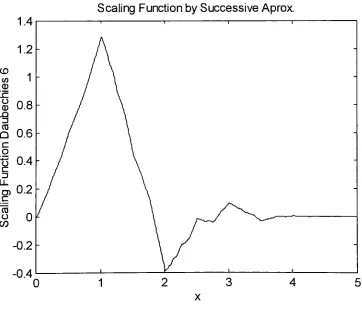
Daubechies

also states

that

if

only

a

finite

number of

the

ak

are

nonzero,

then <p

will

have

compact

support.

Thus,

\<p(x)y/{x-m)dx

=

(-1)V*a*-2

=

k

allows

the translates

of

the

scaling function

and

wavelet

to

define

summable

orthogonal subspaces!

This

will

be

a significant aspect.

Smooth scaling functions

arise

as a consequence of

the

degree

of

approximation

of

the individual translates.

The

conditions

that the

monomials

CHAPTER

3

1

,x,...

,

xp"1

be

expressed as

a

linear

combination

of

the translates

of

tp(x-k)

is

implied

by

the

condition

JV-1

(-1)**X=0

form=0,

1,

...,(N/2)-1.

(3.6)

k=0

The

above equation

is

referred

to

as

the

moment zero condition.

Throughout

these equations,

j

is

the

dilation

parameter or

simply

the

scale.

In

the

approximation

to

solutions

of

differential

equations,

j

is

also

called

the

approximation

level.

For

a

certain

value of

j

and

N,

the

support

of

the

scaling

function

(p(2J

x-k)\s

given as

follows:

~k

N+k-i

supp(<p(2}

x-k))

2

These

three

conditions make

it

possible

to

express

equations

in

the

now

familiar

form:

f(x)

=

Y,2j/2ck<p(2Jx-k)

(3.7)

k

Here it is

worth

emphasizing

that there

are

two

convergence properties used

in

the

above

expansion.

One

is the

uniform

convergence

for

the

level

of

approximation

in

relation

to the

scale

j

and

the

other

is

the

rapid convergence

for

smoother

scaling functions

which

relate

to the

variable

N. These

properties are

not shared at

the

same

time

by

the

usual

classical orthogonal

functions.

The

trade

off

for

the

N

and

j

is very important. The bigger

j

and

N

gives

higher

accuracy

and

faster convergence;

it

also gives a

larger

system of equations and

a

larger

number

of

connection

coefficients needed

to

be

calculated.

A

proper

CHAPTER

3

For

a

better

understanding

of

this,

please

refer

to the

paper

by

Qian

and

Weiss(6)

This

paper goes

into

more

detail

about

this

aspect.

The

authors states

that

a value

greater

than

N=20

should not

be

considered.

By

looking

at

the

error

graphs

in

this

paper

(page

165),

one should not

use

a

Daubechies

wavelet with

N>12.

However,

on page

160,

Qian

and

Weiss(6)

state

that

for

N=6,

the

Daubechies-Galerkin

method

actually

solves

the

Helmholtz

equation

in fewer

operations

than the

dealiased FFT

algorithm

(which

uses shifted grids

to

eliminate

aliasing

terms).

Also,

considering

that

reputable

sources

have

published values

for N=6 Daubechies

wavelet

(or simply

D6)

connection

coefficients

and

moments, I have

chosen

to

perform all

operations

using D6.

CHAPTER

4

Variational Formulation

This

process

begins

with a

differential

equation.

Suppose

you are given

a

differential

equation

defined

over some

boundary

or

interval. We

let the

differential

equation

take the

form

Au

=

f

within

the

boundary

or

interval

where

A is

the

differential

operator

and

the

form

Bu

=

g

on

the

boundary

or

interval

where

B

is

the

boundary

operator.

Let

us

consider

the

problem of

the

following

differential

equation:

d_

dx

a(x)

dx

=

q{x)

for 0<x<L

with

the

following boundary

conditions:

u(0)=u0

and

a

=Q0

\

dxj^

In

these expressions,

a

and

q

are

functions

of

x,

and

u0

and

Q0

are

specified values.

L

is

the

length

of

the

one-dimensional

domain,

u

is

the

dependent

variable.

We

will

take this

problem

to

have

nonhomogeneous

boundary

values,

which means

the

specified values

u0

and

Q0

are not equal

to

zero,

for

arguments sake.

This

type

of equation

may

be

commonly

found in

the

areas

of

heat

transfer

and

fluid

flow,

to

name

only

two

applications.

To

start

the

variational

formulation,

all

the terms

must

be

moved

to

one

side

of

the

equation.

Then,

the

equation

is

multiplied

by

a

function

w called a

test

CHAPTER

4

0=f

Jo

w

dx

f

du~^

a

V

dxj

-q dx

The resulting

equation above

is

called

the

weighted-integral

or

weighted-residual

statement.

The

expression within

the

brackets may be

called

the

residual.

Since

the

function

w

is

called

the

weight

function,

it is easy

to

see

where

the

term

"weighted-residual"

came

from. The

residual

does

not equal

zero when replaced

by

its

approximation.

The

weight

function is any function

that

is

zero on

the differential

boundary

and such

that the

integral

makes

sense.

In

essence,

it

can

be any

nonzero,

integrable function.

The

second

important step is

to

integrate

the

first

term

of

the

expression

by

parts.

Recall

that

integrating by

parts

is simply

using the

equivalent

expressions

below.

rb

p rb wdv =

\wv\

-vdw

rL

At any

rate, the

expression

0=

\

w

dx

(

du^

a

v.

dxj

-q dx

becomes

rf

dw

du

\

. a

wq

ax-i\dxdx

J

wa-

du

~dx

=

0

Notice

that

the

weight

function

is

required

to

be differentiable

at

least once,

ruling

out

constants

as

valid

weight

functions.

Of

special

note, this

is

called

the

weak

form

of

the

original

differential

equation.

"Weak"

refers

to the

reduced

(i.e.,

CHAPTER

4

weakened)

continuity

of

u,

which

is

required

to

be

twice-differentiable

in

the

weighted

integral

form,

but only

once-differentiable

in

the

weak

form.

Boundary

conditions should

be

given

some

attention now.

Boundary

conditions are of

two types:

natural

or

Neumann

and

essential or

Dirichlet

conditions.

The

following

rule

is

used

to

identify

the

natural

boundary

conditions

and

their

form. After

completing

the

integration

by

parts,

examine

all

boundary

terms

of

the

integral

statement.

The

boundary

terms

will

involve both

the

weight

function

and

the

dependent

variable.

Coefficients

of

the

weight

function

and

its

derivatives in

the

boundary

expressions

are

termed the

secondary

variables

(SV).

Specification

of

secondary

variables on

the

boundary

constitutes

the

natural

boundary

conditions

(NBC).

For

this example, the

boundary

term

is

w(a

du/dx). The

coefficient of

the

weight

function is

a

du/dx.

Therefore,

the

secondary

variable

is

of

the

form

a

du/dx. The secondary

variables

always

have

physical

meaning,

and are often quantities of

interest.

The

dependent

variable

of

the problem,

expressed

in

the

same

form

as

the

weight

function

appearing in

the

boundary

term,

is

called

the

primary

variable

(PV),

and

its

specification

on

the

boundary

constitutes

the

essential

boundary

conditions

(EBC).

Above,

the

weight

function

appears

in

the

boundary

expression

as w.

Therefore,

the

dependent

variable u

is

the

primary

variable,

and

the

EBC involves specifying

u

at

the

boundary

points.

It

should

be

noted

that the

number and

form

of

the

primary

and

secondary

variables

depend

on

the

order of

the

differential

equation.

The

number of

CHAPTER

4

variable

there

is

an associated

secondary

variable.

However,

only

one

of

the

pair

may be

specified at a point on

the

boundary!

The

third

and

last step is

to

incorporate

the

boundary

conditions.

We

require

the

weight

function

w

to

vanish at

the

boundary

points where

the

essential or

Dirichlet

conditions occur.

Accordingly,

the

weight

function

w

is

required

to

satisfy

the

following

conditions

W(0)

=

0,

because u(0)

=

u0

This leaves

our equation of

the

form:

0=f

a

-wq

\dx-w(L)QQ

where

Qt

iiO

du

a

V

dxjx=L

J0\dx

dx

J

This

completes

the

development

of

the

weak or

variational

form

of a

differential

equation.

CHAPTER

5

Approximation

Methods to the

Variational

Form

To

solve

the

variational

form,

we will

use

an

approximation.

This

will

be

done

out

of

necessity

basically.

For large

or

hard

problems,

an exact

solution

may be overly difficult. On

a

Global

level,

the

variational

form may be

solved

using

the

Rayleigh-Ritz

method.

It

also

may be

solved

on

a

local level using

what

is

called a weighted residual method.

These

methods

include the

Galerkin,

Least

Squares,

and

Collocation

methods.

This

paper will

focus

on

the

Galerkin

method.

In any

case,

we will

make

the

following

assumption:

ii=

*

=

,<:,

(5.1)

n

This

says

that the

exact solution

u

is

approximated

by

u*

which

is

equal

to

the

summation of

approximation

functions

OF)

multiplied

by

constants

(c). This

summation

may

now

be

substituted

into

the

variational

form.

Since

u*

is only

an

approximation

of

u, the

resulting Residual

equation

is

not equivalent

to the

equation

into

which

it

was

substituted.

That is why

the

Residual does

not equal

zero,

as

mentioned

in

the

earlier section.

In

order

for

an

approximation

technique to

be

considered

Galerkin,

the

weight

function

w

in

the

variational

form

must

be

exchanged

with

W. *F is

sometimes referred

to

as

a shape

function.

This

simple

fact that vF=w is

what

separates

the

Galerkin

method

from

other methods.

The

solution

to the

Galerkin

method

is found

by

solving

the

CHAPTER

5

the

exact

solution,

at

the

points where a solution

is found. With

this

knowledge,

it

is

easy

to

see

why

the

Galerkin

method

has

gained

so much

popularity

over

the

past

fifty

years.

As

stated

above,

shape

functions

are

function

approximations.

In

variational

methods,

the

shape

function

must

fulfill

certain requirements

in

order

for

the

approximation solution

u*

to

be

convergent

to the

actual

solution u as

the

number of elements

increase. These

are:

1

.

The

approximate solution should

be

continuous over

the element,

and

differentiable.

2.

It

should

be

a complete

polynomial,

i.e.,

include

all

lower-order

terms

up

to

the

highest

order

used.

3.

It

should

be

an

interpolant

of

the

primary

variables

at

the

nodes of

the

finite

element.

CHAPTER 6

Galerkin

Method

The Galerkin

Method

is

a

weighted

residual

method

of

approximating

solutions

to

differential

equations.

The Least Squares

Method

and

Collocation

are

also

weighted

residual

methods,

however,

we

will

be

focusing

on

the

Galerkin

method.

It is

an

incredibly

accurate method

that

has

gained

popularity

during

the

past

fifty

years.

The

actual

variables

that

will

be

solved

for

(displacement for

a structural

problem, temperature

for

a

thermal

problem,

etc..)

are

pinpoint accurate

with zero percent

difference!

It

is this

aspect which makes

the

Galerkin Method

so

well received.

As

stated

above, the

Galerkin Method is

a

weighted residual method.

The

first step

of

the

method

is to

make

a

substitution

for

whatever

variable

the

functional

is

in

terms

of.

For

instance,

if the functional

is in

terms

of

u,

and

f is

a

function

of

x,

L(u)

+

f=0

(6.1)

We

must make

a

substitution

for

all u's

as

follows:

I/ =* ₌

2^W-(eqn5.1)

where

u*

is

an

approximation

of

u,

%

is

called

the

shape

functions

and

Uiare

the

values

of

the

solution.

Shape functions

are

function

approximations.

Now,

the

Residual,

R,

is

as

follows:

R

=

CHAPTER

6

To

get

a

solution

to the

problem,

we

must

multiply R

by

a

weighting

function,

Wj(x),

and

integrate

over

the

element

size,

h,

and

set

this

equal

to

zero.

h

\w,(x)Rdx

=

0

i=l,2,3,...,n

(6.4)

0

However,

for

Galerkin

Method, Wj(x)

=

%{x).

Now,

Integrate

n

times

per

element.

The

number n

will

be determined

by

the type

of

shape

function

used.

The

resulting

equations will need

to

be

assembled

in

a master

equation which

will

take the

form

[A](U0

=

(F)

The

matrix

A

will

be

a

square

matrix.

The

solution

vector

(Ui)

may be

found

now

using

standard

Linear Algebra

techniques

and whatever

Boundary

Conditions

exist

in

the

problem.

Take

as an example

the

differential

equation:

3U"+4U'-5x

=

0

0<x<L

The

primes

that follow the

variable

denote the

derivative

with

respect

to

displacement.

ir=du_tU,t=(dir

dx

dx\dx

_j

Therefore,

tf

=

(34Vc7J+(42X<y,)-5x

*

0

Following

the

procedure,

\WlRdx

=

r),W]

=

XJ

This is

what

distinguishes

the

Galerkin

method

from

other

weighted-residual

methods.

CHAPTER

6

\W]3(Yd%'Uiydx

+

\^j4(^l'Ui)dx

=

]^j5xdx

0 0 0

Now,

the

equation

is ready

to

be

solved.

The first

term

on

the left

side of

the

equation

must

be

integrated

by

parts.

The

term

on

the

right

must

be

evaluated at x

=

xk

+

x,

where

xk

is

a constant.

This

means

that the

constant

term

will

change as

the

elements progress.

In

other

words,

xk

will

equal

the

previous

xk

plus element size

h.

Each

element

will

have its

own set

of equations.

A

Global

equation must

be formed

by

assembly

of

the

element

equations.

As

stated

earlier,

standard

Linear Algebra

techniques

may be

used

to

solve

for

the

values

of

U.

The

requirements

for

shape

functions may be found

on page

25

in

Chapter Four. There

are

three

common

types

of

shape

functions

which

satisfy

these

requirements.

They

are

linear,

quadratic,

and

cubic

hermite.

Linear

elements

have

two

equations

per element

(n=2)

and are affected

only

by

two

nodes.

The

nodes

are on opposite

sides

of

the

element.

This

makes

straight-line

approximations.

The quality

of

the

results

will

be

more

dependent

on

the

number

of

elements

(the

more elements

the

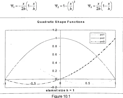
better). The

Quadratic

elements

make

use

of

three

nodes

(n=3).

The

nodes are

located

at

the

beginning,

middle,

and end

of

the

element.

The

three

nodes provide

for

smoother

fitting

of

the

approximation.

Cubic

Hermite

uses

four

equations

(n=4).

However,

there

are

two

nodes

located

at

the

beginning

and

the

end

of

the

element.

At

each node

there

are

two equations,

one

for

position

and one

for

slope.

This

makes

for

a

CHAPTER

6

elements will

give

the

same

precise values at

the nodes,

but

the different types

will give

progressively better

results

between

the

node