Predicting Visual Memory Schemas with Variational Autoencoders

Autoencoders.

White Rose Research Online URL for this paper:

http://eprints.whiterose.ac.uk/151860/

Version: Accepted Version

Proceedings Paper:

Kyle-Davidson, Cameron Philip, Bors, Adrian Gheorghe orcid.org/0000-0001-7838-0021

and Evans, Karla orcid.org/0000-0002-8440-1711 (2019) Predicting Visual Memory

Schemas with Variational Autoencoders. In: Proc. British Machine Vision Conference

(BMVC). .

[email protected] https://eprints.whiterose.ac.uk/ Reuse

Items deposited in White Rose Research Online are protected by copyright, with all rights reserved unless indicated otherwise. They may be downloaded and/or printed for private study, or other acts as permitted by national copyright laws. The publisher or other rights holders may allow further reproduction and re-use of the full text version. This is indicated by the licence information on the White Rose Research Online record for the item.

Takedown

If you consider content in White Rose Research Online to be in breach of UK law, please notify us by

Predicting Visual Memory Schemas with

Variational Autoencoders

Cameron Kyle-Davidson*

[email protected]

Adrian G. Bors*

[email protected]

Karla Evans**

[email protected]

*Dept. of Computer Science *YO10 5GH

**Dept. of Psychology **YO10 5DD

University of York York, UK

Abstract

Visual memory schema (VMS) maps show which regions of an image cause that im-age to be remembered or falsely remembered. Previous work has succeeded in generating low resolution VMS maps using convolutional neural networks. We instead approach this problem as an image-to-image translation task making use of a variational autoencoder. This approach allows us to generate higher resolution dual channel images that repre-sent visual memory schemas, allowing us to evaluate predicted true memorability and false memorability separately. We also evaluate the relationship between VMS maps, predicted VMS maps, ground truth memorability scores, and predicted memorability scores.

1

Introduction

Determining capacity and the nature of visual memory has been a focus of psychological experiments for decades. However, it is only recently thatmemorability has been able to be defined and predicted using computational methods. This definition of memorability has been found to be separate to other commonly computed image factors such as saliency or interestingness. The basis of this definition in prior work is related to the hit rate (HR) of an image, which is how well a target image is recognised after being repeated in a sequence of images. Predicting the memorability score for an image representing how likely a given image is to be remembered by a human during a recognition test, is a difficult task - memo-rability has been shown to be associated with the semantic content of the image, a complex dimension to extract. With the advent of large memorability datasets that contain tens of thousands of images paired with ground truth memorability scores, recent deep learning models’ have succeeded in achieving close-to-human performance in predicting how likely an image is to be remembered.

Previous work in the arena of memorability prediction has been engineered with the goal of predicting memorability scores for a given image. Few research studies explored creating models capable of predicting the regions of an image that contribute the most to an image’s memorability. These models’ predictions of memorable regions lack a clear relation to the ground truth, as until very recently no dataset of the regions that causehumans to find a

c

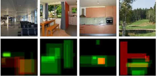
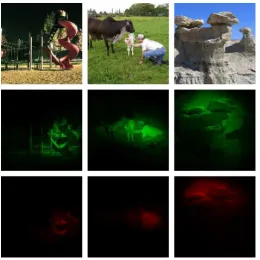
given image memorable, existed. A new image memorisation dataset was introduced in [1] which tackles this problem by introducing theVISCHEMAimage dataset, which contains human indications of what regions made them remember certain images. Moreover, a new concept known as Visual Memory Schema (VMS), which associates for each image in the dataset two dimensional probability density functions (PDF) that represent which areas of that image cause to be either remembered (a true VMS map), or falsely remembered (a false VMS map). Examples of the VMSs are shown on the second row in Fig.1, corresponding to the images from above. According to the experiments, such VMS maps have been shown to be consistent between people. By following certain psychology studies it was hypothesised in [1] that these regions correspond to mental structures that aid remembering.

Figure 1: Examples of images and their corresponding VMS maps. In the second row of images, red areas correspond to regions that cause the associated image to be falsely remem-bered, while green regions are responsible for correctly remembering the image. Falsely remembered regions cause a person to believe they have seen the given image when in fact, they have not.

We hypothesise that a relationship exists between images that have strong, either true or false VMS maps, and seek to learn this relationship to better understand the meaning of the VMS maps and the relation between memorability and false memorability. More specifically, we expect that memorable images align along dimensions of ‘memorability’ and likewise for false memorability. Learning a structured embedding in this ‘memorability space’ would lead to the capability to generate both true and false VMS maps for unseen images, and hence aid understanding of which mental structures contribute to remembering or falsely remembering an image. We approach this problem via Variational Autoencoders (VAE) models, which have previously been shown to be capable of learning to group similar data in an unsupervised fashion by mapping through a latent space. We hence pose the problem of learning such transformations, and the resulting VMS map generation, as an image-to-image translation problem.

use VAE for learning VMS maps, Section5presents the experimental results and Section6

draws the conclusions of this study.

2

Relevant Work

2.1

Predicting the memorability of images

Predicting how likely an image is to be remembered is a problem that has only recently be-come an active area of interest in computer vision. Isolaet al. created an initial memorability dataset of over 2000 images and experimented with using certain feature extractors paired with a support vector machine (SVM) for prediction[10]. Isola found that humans generally agree on what is memorable, achieving a consistency of more than 0.68 as measured by the Spearman Rank Correlation metric. In general hand picked features achieve a consistency of less than 0.5. Penget al. [16] and Jinget al. [11] use multiview modelling achieving a consistency with the ground truth greater than that of any SVM based model. Later work by Khoslaet al. improves upon these results, introducing the LaMem dataset [12] of 60,000 images and their corresponding memorability scores. Moreover, they introduced MemNet, a convolutional neural network (CNN), for the purpose of prediction. Fajtlet al. constructed a CNN-LSTM (Long Short-Term Memory) hybrid model known as AMNet that iteratively generates attention-based memorability scores, achieving a performance very close to human consistency [6] when trained upon the LaMem dataset.

2.2

Predicting memorability maps

Relatively little work has examined the generation of memorability maps directly. Khoslaet al. used a probabilistic process to generate memorability maps [13] by considering the re-gions of images that are likely to be remembered or forgotten. The MemNet CNN developed also by Khosla was also capable of creating heatmaps of the most memorable and the least memorable regions of a given image. Similarly, the work of Fajtlet al. iteratively generates attention based memory maps that are concatenated to generate a final score. However, none of these methods would generate memory maps which can be compared with ground truth maps of memorability.

A dataset of 800 scene images and their associated ‘Visual Memory Schema’ (VMS) was developed during the VISCHEMA experiment. The images considered for this dataset are divided through a tree structure, where each level describes a certain aspect of that image in increasing detail. Images are first divided intoindoorandoutdoor. Theindoorcategory contains the categoriesprivateandpublicwhile theoutdoor category containsman-made

andnaturalimages. These are further subdivided, withprivatecontainingkitchenandliving room,publiccontainingsmallandbig(which refers to the size of the public space shown in the image). Theman-madecategory containswork/homeandpublic entertainmentand the

3

Variational Autoencoders

Autoencoders (AE) attempt to learn efficient latent-space encodings of the input data that would allow its reconstruction from such an encoding. A variational autoencoder (VAE) [14] is an extension of the AE, which has the training aim to maximise the lower bound of the marginal log-likelihood of the data following encoding and reconstruction. This means minimising the KL divergence between the posterior anda prioridata distributions during the training. Rather than just learning a compressed encoding of the data, a VAE learns a probability distribution that is an approximation of the true probability distribution of the underlying data. This allows a VAE to be used as a generative model based on sampling in the latent space.

VAEs are made up of two components - anencoder which converts input dataxinto a latent space representationz, and adecoderthat converts a latent space variablezback into datax′ akin to the inputx. CNNs are used for implementing both the encoder and the decoder. The encoder is defined as a probabilistic machineqθ(z|x)that extracts a specific latent space codezwhereθrepresents the parameters of the encoder’ network. Meanwhile, the decoder maps the information in a probabilistic sense defined bypφ(x|z)in the opposite way from the codezback to the data spacex, whereφdefined the parameters of the decoder network. The encoder and decoder are related through the loss function which consists of two components:

L(θ,φ) =−E_z∼q

θ(z|x)[logpφ(x|z)] +KL(qθ(z|x)||p(z)) (1)

whereKL(·)represents the Kullback-Liebler divergence between thea prioridistribution of the latent spaceqθ(z|xi)and its estimated distributionp(z). The first term from equation (1) represents the reconstruction loss and the second term regularises the learnt distribution. The latter term helps the VAE to learn to group conceptually similar data in the same regions of the latent space.

4

Generating Visual Memory Schemas using VAEs

The aim of this research study consists in developing a generative method for Visual Mem-ory Schemas (VMS), for a given input image. In our approach we would aim to generate both true and false VMSs, simultaneously. This is defined as an image-to-image translation problem by making use of an VAE consisting of two CNNs, with the first one, the encoder designed to learn a mapping from an image to a latent code, while the decoder to learn the mapping from that latent code to a VMS. Previous work [7,15] has shown that CNNs work well at extracting high-level image features that also allow for the prediction of memorability [2]. CNNs such as VGG-16 network have also been shown to be capable of learning to re-construct VMS maps at some degree for certain image categories [1]. We propose using VAE models which have good ability to learn data classification in the latent space, as exemplified in Fig.2. This model would allow a good separation of the false and positive VMS encoding spaces and then for the generation of dual channel VMS maps for generic scene input images corresponding to true and false VMS structures in which given random memorable images produce latent codes similar to those indicated experimentally by humans in memorable im-ages. Moreover, the learned latent space modelled by VAEs can be easily inspected in order to find relations between the memorability and false memorability of images.

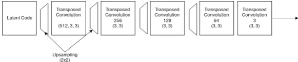
Figure 2: Predicting VAEs in images using an autoencoder.

layers. The final output of the VGG architecture will be connected to a dense layer in order to compress the representation further, followed by the latent encoding. In CNNs the deep features that would emerge capture structures of the objects in the scene [18] and semantic structures [8] present in the input image.

The decoder would usually be simpler than the encoder. Whereas the input of the encoder consists of real world scenes, the output of the decoder is a VMS map, which consists of only two channels representing the spatial density of how likely a given image region is to cause that image to be remembered. There is no benefit in using a very deep architecture for the decoder, as we do not need to recreate any meaningful semantic features in the output. Additionally, a simpler architecture keeps the number of trainable parameters low, which is important when considering the low amount of available training data.

The loss function for this model is similar to the standard VAE loss function from (1), with the exception that in the reconstruction term, instead of reconstructing the original

image data, aims to reconstruct associated information, such as VMSs. If X is the set of scene images andY the set of associated VMS maps, withx∈X andy∈Y representing corresponding images drawn from these sets, our loss function is:

L=−E_z∼qφ(z|x)[logp_Ψ(y|z)] +KL(qθ(z|x)||p(z)) (2) whereΨrepresents the parameters associated with the VAE reconstructing the VMSs datay

at the end of the encoder. We additionally investigate replacing the reconstruction term with the l1-norm as in [1].

5

Experimental results

5.1

Experimental Setup

For the encoder we use a pretrained VGG-16 network to extract a 7×7×512 representation of an image, then compress this further using an n dimensional dense layer, which leads to a latent space with a dimension of m. All parameters of the VGG network are frozen, by considering learning rates set to 0 during training, to avoid damaging the deep features while training on a small dataset such as ours. We employ data augmentation for training due to the small size of the training set. Data augmentation involves various realistic image manipulations, such as for example shifting the image either horizontally or vertically by 0.1 of the total image width, zooming the image, and horizontal flipping, for increasing the training data.

The decoder consists of a five layer upsampling network, shown in Fig.3, that imple-ments transposed convolutions in order to convert them-dimensional latent variable space back into an image. We apply batch normalisation after every convolution and employ l2 kernel regularisation [4], l = 0.02, and a learning rate of 0.0001. We use a batch size of 32 and train the network for 250 epochs with 20 steps per epoch. In the experiments we evaluate three different architectures considering: 1) n = 64 and m=8; 2) n = 64 and m=8 with anl1 reconstruction loss; 3) n = 128 and m=32. The input and output of the entire architecture is a 224×224 image. The model is implemented in Keras1.

5.2

Datasets

We evaluate the network over three datasets:

1. VISCHEMA. The dataset2used in [1]. Consists of 800 images and 800 Visual Mem-ory Schemas taken experimentally on a group of 100 people who were asked to indi-cate whether they remember certain images and if yes, to indiindi-cate what image regions made them remember them. This dataset is divided into a 640 image training set and a 160 image test set.

2. VISCHEMA2. A new set of scene images extracted from the FIGRIM dataset, and divided into the same hierarchical structure as the original VISCHEMA dataset. No ground truth visual memory schemas are available yet for this dataset, but because the categories and semantic content of the images are highly similar with the original dataset, VISCHEMA2 is useful for evaluation purposes.

3. LaMem. A dataset of 60,000 images, of a wide variety, with corresponding ground truth memorability scores [12].

5.3

VMS reconstruction

We evaluate reconstruction results of the original VISCHEMA dataset using both standard mean squared error (MSE) over all test images and the two dimensional Pearson product-moment correlation coefficientsρ2D_{. We average the results on all true VMSs, and false}

VMSs, separately. True VMSs represent the VMS map regions indicated by participants in the experiments that represent what made them remember that image, while false VMSs rep-resent regions from images, falsely indicated by people that made them remember those im-ages. Actually those images have not been shown to them before. We obtain this metrics for all visual schemas and then evaluate the relation between this metric and the more standard ‘memorability score’ provided in the LaMem dataset [6]. The relationship between visual memory schemas and computational saliency is also explored. Computational saliency maps for the VISCHEMA datasets are generated via the Graph Based Visual Saliency (GBVS) al-gorithm [9].

Finally, we employ a state-of-the-art memorability prediction network and evaluate the relation between the VISCHEMA datasets memorability scores of the predicted VMS and the VMSs corresponding to the choices made by people, for both datasets, VISCHEMA and the VISCHEMA2. For all evaluations of our memorability metrics and standard memorabil-ity scores we follow prior work from [10], [12] and use Spearmans rank correlation.

1_{https://keras.io}

Latent Space VMS ρ2D MSE Dimension (m)

32

True 0.545 92.54 False 0.369 70.526 All 0.57 85.379

8

True 0.513 90.812 False 0.333 64.228 All 0.53 83.472

8 and L1 norm in (2)

True 0.543 72.348 False 0.168 25.131 All 0.559 72.052

Table 1: Reconstruction accuracy for three deep learning architectures.

Table1shows the reconstruction results in terms of both MSE and Spearmans rank cor-relation,ρ2D. The network with an m=8 dimensional latent space and an l1-norm component to its loss function has the overall best MSE, while the network with the overall best Pear-sons correlation with the ground truth is the network with a m=32 dimensional latent space. Our overallρ2D _{results are slightly worse than those presented in [1], though it should be}

noted that we generate both the true and false maps simultaneously. This allows us to inves-tigate how well the individual true and false VMS are reconstructed. In general, false VMS maps are more difficult to accurately reconstruct than true VMS maps. This is likely due to the overall lower consistency between human observers for false VMS maps. While what is memorable tends to be well agreed on among people, what causes false remembering of an image is more varied, and this effect crosses over to generative models. Interestingly, we find that a higher dimensional latent space has the best effect on reconstruction accuracy, rather than the use of an l1-norm in the loss term. This is due to the effect of the second term in the loss function from equation (2) and indicates that higher dimensional spaces are better at capturing ‘memorability’. For the rest of this section we evaluate the results of the network with am=32 dimensional latent space, given that this architecture performs the best as measured by theρ2Dmetric.

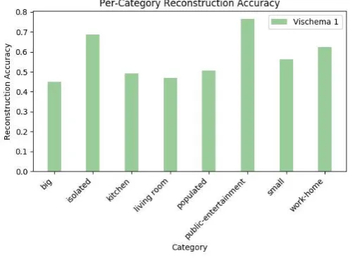
Figure4shows the reconstruction accuracy measured byρ2D for each category in the VISCHEMA dataset, over the 160 image test set. We find that the best performing category is that of Public Entertainment, with a correlation of 0.766, which is better that the results from [1] which found that the Work-Home image category had the best performance with a correlation of 0.677. A comparison with prior work is shown in Table2.

Work Best Category ρ2D Worst Category ρ2D Overallρ2D

Previous Method Work/Home 0.677 Living Room 0.506 0.588 Our Method Public Entertainment 0.766 Big 0.449 0.57

Table 2: Comparison with Prior Work

The worst performing category for VMS reconstruction is the "Big" which contains im-ages of airport terminals with a correlation of 0.449. In general, we find that categories that have high overall memorability tend to reconstruct better than the categories with low overall memorability. Differences from prior work may also be due to generating higher res-olution images, which captures more detail in some categories yet causes more divergence in categories with less available memorability information. We found that the correlation between predicted VMS maps and saliency maps, provided by GBVS algorithm [9], to be 0.69 which agrees with other results on the relationship between memorability and saliency

[1,5]. GBVS is a well used saliency measure, but VMS maps offer more than saliency alone. When averaging on all image categories and comparing with saliency, we found that false VMS maps have a correlation of 0.625 while true VMS maps have a correlation of 0.704.

5.4

Memorability results

(a) VISCHEMA2 (b) VISCHEMA

Figure 5: Comparison of the memorability results for a set of image categories between the VISCHEMA2 and VISCHEMA datasets.

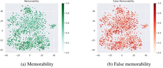
of the Memorability and those corresponding to False Memorability, shown in Fig.6a and

6b, respectively. Images that tend to be highly memorable also tend to be highly falsely memorable. In Fig. 7, three images from VISCHEMA2 are shown on first line and their corresponding true and false VMSs are shown on second and third line, respectively.

(a) Memorability (b) False memorability

Figure 6: VISCHEMA2 Latent Space Embedding. Green represents memorability and red represents false memorability, normalised between 0 and 1.

5.5

VMS Maps and Memorability Scores

Predicted memorability scores for both VISCHEMA 1 and 2 datasets were obtained by em-ploying the AMNet network [6]. These scores were then compared to the memorability metric used for evaluating visual schemas. No significant relationship was found between the per-category memorability metrics and the predicted category memorability scores aside from VISCHEMA2’s "Populated" category which had a Spearmans rank correlation with the AMNet scores of 0.203 with p<0.01. It appears that VMSs, even predicted schemas, do not directly relate to predicted memorability scores for the same images, and that unlike our VMS prediction model, predicted memorability scores may not take fully into account what humans find memorable. It has been shown that deep neural networks take the simplest approach possible to solving a problem [3], and it is possible that memorability prediction models are working on factors that do not necessarily align directly with memorability if some other learned metric provides a ‘good enough’ approximation. This could explain why predicted scores do not align with VMS maps.

We also examine the relationship between the ground truth memorability scores and our metric by predicting VMSs for a 10,000 image subset of the LaMem dataset, used in [6], and estimating only the true memorability score for them. We then use the Spearmans rank to compare the ground-truth score and our metric. We find a rank correlation of 0.147 withp<0.01, indicating that VMS maps and experimentally-based memorability scores are weakly, but significantly, related.

6

Conclusion

Figure 7: Set of three images from VISCHEMA2 dataset and their predicted true VMS and false VMS on second and third lines.

metrics and the predicted per-category metrics, and finally show that current state-of-the-art memorability prediction does not appear to correlate with ground truth or predicted VMS metrics, and that these metrics do have a significant, but weak, positive correlation with ground truth memorability scores from the LaMem dataset. This indicates that VMSs can provide additional information about image memorability which is not traditionally captured by other memorability prediction methods.

7

Acknowledgements

The first author would like to acknowledge the support from the Doctoral Training Grant provided by the EPSRC.

This project was undertaken on the Viking Cluster, which is a high performance com-pute facility provided by the University of York. We are grateful for computational support from the University of York High Performance Computing service,Viking and the Research Computing team.

References

[1] E. Akagunduz, A. G. Bors, and K. K. Evans. Defining Image Memorability using the Visual Memory Schema. IEEE Trans. on Pattern Analysis and Machine Intelligence (PAMI), 2019. URLhttp://arxiv.org/abs/1903.02056.

[3] W. Brendel and M. Bethge. Approximating CNNs with Bag-of-local-Features models works surprisingly well on ImageNet. InProc. Int. Conf. on Learning Representations (ICLR), 2019. URLhttps://arxiv.org/abs/1904.00760.

[4] Corinna Cortes, Mehryar Mohri, and Afshin Rostamizadeh. L2 regularization for learn-ing kernels.CoRR, abs/1205.2653, 2012. URLhttp://arxiv.org/abs/1205. 2653.

[5] R. Dubey, J. Peterson, A. Khosla, M. Yang, and B. Ghanem. What makes an object memorable? InProc. IEEE Int. Conf. on Computer Vision, pages 1089–1097, 2015. [6] J. Fajtl, V. Argyriou, D. Monekosso, and P. Remagnino. AMNet: Memorability

Estima-tion with AttenEstima-tion. InProc. IEEE Computer Vision and Pattern Recognition (CVPR), pages 6363–6372, 2018.

[7] D. Garcia-Gasulla, F. Parés, A. Vilalta, J. Moreno, E. Ayguadé, J. Labarta, U. Cortés, and T. Suzumura. On the Behavior of Convolutional Nets for Feature Extraction.Jour. of Artificial Intelligence Research, 61:563–592, 2018.

[8] A. Gonzalez-Garcia, D. Modolo, and V. Ferrari. Do Semantic Parts Emerge in Convo-lutional Neural Networks? Int. Journal of Computer Vision, 126(5):476–494, 2018. [9] J. Harel, C. Koch, and P. Perona. Graph-Based Visual Saliency. InProc. Advances in

Neural Information Processing Systems (NIPS), pages 545–552, 2006.

[10] P. Isola, J. Xiao, A. Torralba, and A. Oliva. What makes an image memorable? In

Proc. IEEE Conf. on Comp. Vision and Pattern Recognition, pages 145–152, 2011. [11] P. Jing, Y. Su, L. Nie, and H. Gu. Predicting Image Memorability Through Adaptive

Transfer Learning From External Sources. IEEE Trans. on Multimedia, 19(5):1050– 1062, 2017.

[12] A. Khosla, A. S. Raju, A. Torralba, and A. Oliva. Understanding and Predicting Image Memorability at a Large Scale. InIEEE Int. Conf. on Comp. Vision, pages 2390–2398. [13] A. Khosla, J. Xiao, A. Torralba, and A. Oliva. Memorability of image regions. In

Advances in Neural Information Processing Systems (NIPS), pages 296–304, 2012. [14] D. P. Kingma and M. Welling. Auto-Encoding Variational Bayes. InProc. Int. Conf. on

Learning Repres. (ICLR), 2014. URLhttp://arxiv.org/abs/1312.6114. [15] J. Lukavský and F. Dˇechtˇerenko. Visual properties and memorising scenes: Effects of

image-space sparseness and uniformity. Attention, Perception, & Psychophysics, 79 (7):2044–2054, October 2017.

[16] H. Peng, K. Li, B. Li, H. Ling, W. Xiong, and W. Hu. InProc. of the 23rd ACM Int. Conf. on Multimedia, pages 1147–1150, 2015.

[17] K. Simonyan and A. Zisserman. Very Deep Convolutional Networks for Large-Scale Image Recognition. 2014. URLhttp://arxiv.org/abs/1409.1556.

[18] B. Zhou, A. Khosla, A. Lapedriza, A. Oliva, and A. Torralba. Object Detectors Emerge in Deep Scene CNNs. InProc. Int. Conf. on Learning Representations (ICLR), 2015.