Corrosion Inhibition Efficiency of Thiophene Derivatives on Mild Steel: A QSAR Model

Int. J. Electrochem. Sci., 9 (2014) 1678 - 1689

International Journal of

ELECTROCHEMICAL

SCIENCE

www.electrochemsci.org

Corrosion Inhibition Efficiency of Thiophene Derivatives on

Mild Steel: A QSAR Model.

Bishir Usman1,2,Hasmerya Maarof1, Hassan H. Abdallah1,Rosmahaida Jamaludin, Abdo M. Al-Fakih1, Madzlan Aziz1*

1

Department of Chemistry, Faculty of Science,Universiti Teknologi Malaysia, 81310 UTM. Skudai, Johor Bahru, Malaysia,

2

Department of Pure and Industrial Chemistry, Bayero University, Kano.P. M. B. 3011, Kano, Nigeria. *

E-mail: madzlan@utm.my; bishirbum@yahoo.com

Received: 25 November 2013 / Accepted: 30 December 2013 / Published: 2 February 2014

A quantitative structure activity relationship (QSAR) model was built using Interval Partial Least Squares and Partial Least Squares (IPLS-PLS) regression for the prediction of corrosion inhibition efficiency of thiophene derivatives. Eleven compounds with their activity expressed as percentage inhibition efficiency (%IE) were obtained and divided into a training set (ntrn = 7) and test set (ntes= 4). Molecular descriptors were generated using Dragon software and the important relevant descriptors were selected using an objective variable selection followed by subjective variable selection using IPLS. Several models were built using PLS regression and the models were evaluated using statistical significance characterization, r2 and root mean square error calibration (RMSEC). The robustness, accuracy and predictive ability of the models were carried out using external and internal cross validation using regression coefficient cross validation (r2cv) and regression coefficient prediction (r2pred). The values were calculated and found to be > 0.5 and 0.8 respectively for the first and second model and for the external validation the values are found to be > 0.6 and 0.5 respectively and the r2 value was found to be > 0.9. Application of the built model to calculate the theoretical %IE was obtained and is closer to the %IE experimental. The result showed the predictive ability of the model was good and can be used to design a similar group of compounds with corrosion inhibition efficiency.

Keywords: Thiophene, QSAR, IPLS, PLS, %IE, mild steel, corrosion inhibitor

1. INTRODUCTION

act by adsorption on the metal surface and forming a layer as complexes with the metal atom and protect the metal from corrosion [3,4, 5].

Experimental methods are costly, time consuming and can produce toxic site products. The most common methods used in computational chemistry to study corrosion is a quantum chemical calculation using molecular and electronic property of a molecule [6].

The use of corrosion inhibitors for corrosion protection attract many researchers into the area for a number of decades to find a lasting solution to this important global problem, and therefore, a lot of research have been reported on the use of inhibitors to minimize or stop corrosion by theoretical approach. El Ashry and Senior, studied the corrosion activity of lauric hydrazide and its salts as corrosion inhibitors using quantum chemical calculation and QSAR the result revealed the effect of inclusion quantum chemical parameters to improve corrosion inhibition efficiency [7].

Khaled, reported on the corrosion inhibition of 1,3-Pyrimidine derivatives as corrosion inhibitors using genetic algorithm and QSAR model technique the activity of this compound show similarities with experimental [8]. Corrosion inhibition efficiency phenethroline derivatives were investigated by Obot et al., the result shows that protonated specie of inhibitors give better experimental inhibition efficiency [9]. Inhibition and adsorption efficiency of cysteine, glycine, leucine and alanine on mild steel in hydrochloric acid was investigated and the result define the effect of various concentration of the amino acid inhibited the corrosion of mild steel and the correlation between the theoretical obtained from (QSAR) with experimental was found to be excellent [10].

However, Masoud et al., explained the inhibition performance of aminopyridine as corrosion inhibitor using quantum chemical calculation the correlation was found to be good between the theoretical and experimental corrosion inhibition [11]. Therefore the most effective way to obtain a complete set of data without necessarily performing an experiment is the application of quantitative structure activity relationship (QSAR) [12,13]. Once QSAR model is established the activity of the molecules can be predicted and know which structural features play a significant role in the activity. Advances in QSAR model have lead to the search of more potential corrosion inhibitors and their mechanism for corrosion inhibition. Many methods such as multiple linear regression (MLR), partial least square (PLS), heuristic method (HM) and different types of artificial neural network (ANN) which can be applied for QSAR model development and can be used in predicting the corrosion inhibition efficiency, using QSAR model can predict with confidence some experimeally unknown properties which relate molecular structure to specific property.

2. MATERIALS AND METHOD

2.1. Data

A data set of the compounds which consists of eleven thiophene derivatives as corrosion inhibitors were obtained from the literature [15]. The chemical structure and percentage corrosion inhibition are presented in Table 1.

Table 1. Thiophene derivatives with Percentage inhibition efficiency

Compounds structure %IE Experimental Compounds structure %IE Experimental S O O 2-Thiophenemethylester 79.7 S O HO 2-thiophenecarboxylic acid 62.1 S O

H3C

2-acetylthiophene 78.3 S Cl 2-chlorothiophene 60.4 S Br 2-bromothiophene 73.5 S 2-methylthiophene 60.2 S Br 3-bromothiophene 68.9 S 3-methylthiophene 55.5 S HO 2-hydroxythiophene 68.4 S Thiophene 35.5 S O 2-thiophenecaboxaldehyde 67.1

The data on the compound are arranged in order of increasing inhibition efficiency and split into training and testing set in the ratio of 3:1, the splitting is done by choosing every third compound as the test set. The training set and the test compound are stored as a 2D and 3D structure in the computer [16].

2.2. Descriptor Generation and Calculation

[16]. The descriptors were calculated using Dragon-software 6.0 [17]. A total of 2217 descriptors was generated after the calculation using the whole block from the dragon software.

2.3. Feature Selection

The data size is reduced by selecting the most informative descriptor from the pool of data that are used for prediction and building an accurate model. The minimal number of descriptors that are informative were retain and therefore all the data containing redundant information were removed by objective and subjective variable feature selection.

2.4. Objective Feature Selection

Objective feature selection was carried out in order to remove all the descriptors by pairwise correlation matrix , therefore descriptors with high correlation values greater than 0.95 were removed and descriptors with constant values or poor correlation values were discarded and descriptors with zero or missing value were also remove and the descriptor that are not informative were reduced manually which bring the number of descriptors to 250. Finally the descriptors need to be reduced further in order to get robust and accurate QSAR model by subjective feature variable selection using statistical analysis by IPLS stepwise variable selection [18].

2.5. Subjective Feature Selection

The dependent variable was used to select the descriptors that are highly informative in the data set, since iPLS is a method of graphical orientation for local regression modeling of a data. Interval Partial Least Square (IPLS) was used to reduce the data set size, IPLS algorithm was applied to the data contain 7 training set with 250 descriptors , the best interval was selected as described elsewhere [14, 19]. The descriptors containing relevant information were selected in order to improve the capability of the PLS model.

The selected descriptors were based on the evaluation of the regression coefficient value on the number of descriptors selected which was started by a small number of descriptors and subsequently added new variables to improve the model regression coefficients until there was no improvement in the model regression coefficient. From the two models 5 and 2descriptors were found to be significant based on the validation coefficient (r2) and root mean square error cross validation (RMSECV) , than descriptors were used to build the model [14,20,21].

2.6. Model Development

Before the analysis the descriptors were auto-scaled to zero unit and the model was built and evaluated using correlation coefficient r2 and root mean square error of calibration , RSMEC. The model with higher value of r2 and lower value of RMSEC is selected as a good model.

The QSAR Model is represented as QSAR equation with the regression coefficient explaining the significance of the individual descriptors in the regression model.

However, the plot of the experimental activity vs predicted activity is represented and explained the activity of calculated and experimental inhibition efficiency in QSAR.

2.7. Model Validation

This is the final step in QSAR model development that involve external and internal validation of the model.The purpose of model validation is to ensure the model is accurate in terms of stability, robustness and predictive ability. Therefore cross validation was employed as an internal validation using leave one out and checked the model thoroughly. For external validation (external test set ) it involves the prediction of the property of interest for compound that are not used in the model building. The statistical output was obtained in terms of leave one out cross validation regression coefficient ( r2 ), regression coefficient cross validation (r2cv) and regression coefficient predict (r2 pred). The higher the value of r2cv the better the model for the prediction and similarly higher value of r2 pred implies the prediction power of the model. The model obtained was used and predicted the feature compound for corrosion inhibitors which will be used for experimental evaluation.

3. RESULTS AND DISCUSSION

QSAR analysis was used to relate the structure activity relationship of different eleven thiophene derivatives as corrosion inhibitors. In this method of analysis the model quality depends on the fitting and prediction ability. In order to build QSAR model and test the model workability, the data are divided into 7 training set which was used in building the model and test set of 4 compounds which was used to evaluate the model built as in Table 1.

The IPLS-PLS analysis was used to generate 2-model with 5 and 2 descriptors respectively based on latent variable (LV). The linear model built using selected descriptors from the training data set were used and obtained the following linear equation. The selected descriptors obtained from IPLS in combination with PLS for the models with five and two descriptors linear equations as represented below.

%IE = -135.541+[-8.4374(SpMAD_L)]+[-6.8488(MATS4M)]

The equation for the IPLS with PLS for the second model with 2 descriptors

%IE = -135.541 + [-9.881 (MATS4M)] + 57.272 (SpMAX3-Bh(m)) (2) r2 =0. 9295, r2cv = 0.8481, r2pre = 0.5114, N= 250

N is the number of compounds, r2 is the square correlation coefficient, r2cv is the square cross-validation coefficients for leave-one-out and RMSEC is the root means error for calibration an prediction respectively .

3.1. Model validation and interpretation

In this study IPLS in combination with PLS was employed in building the model for the structure of thiophene derivatives as corrosion inhibitors more appropriately, application of the PLS method allow the construction of good QSAR equations without over fitting and eliminating most of the variable that lack information. And this method is used in combination with cross validation to obtain the highest number of components [21]. The PLS regression method used was based on SIMIPLS algorithm existed in the PLS Toolbox of Matlab software (Version 7.6.0), in order to obtain the best output based on the regression coefficient for the predicted compound and leave-one –out cross validation model is represented in Table 2. Results show the regression coefficient r2, with a regression coefficient leave one out cross validation r2cv, and RMSEC. The regression coefficient for prediction r2cv and the model with higher value of these coefficients is selected as the best model.Therefore, model 3 and model 2 are considered as the best models and the best linear model equation are obtained from the models.

Table 2. PLS Model output for regression coefficient

Parameters PLS Model With 2 descriptors PLS Model with 5 Descriptors

r2 0.9295 0.9767

r2cv 0.8481 0.4738

r2pre 0.5114 0.6055

RMSEC 3.415 1.967

The selected descriptors obtained from IPLS in combination with PLS for the first model with five descriptors are represented in Table 3. with the equation of the model.

Table 3. Selected descriptors for the first model with 5-descriptors

Descriptors Definition

SpMAD_L Spectral absolute deviation from Laplace

MATS4M Moran autocorrelation of lag4 weighted by Mass

SPMAX3_Bh (m) Largest Eigen values n3 of Burden matrix weighted by mass RDF010S Radial distribution function weighted 010s/ weighted by 1-state R1P R1p – autocorrelation of lag1/weighted by polarizability

Table 4. Selected descriptors for the second model with 2-descriptors

Descriptors Definition

MATS4M Moran autocorrelation of lag4 weighted by Mass

SPMAX3_Bh (m) Largest Eigen values n3 of Burden matrix weighted by mass

The equation for the IPLS with PLS for the second model with 2 descriptors %IE = -135.541+[-9.881 (MATS4M)] + [57.272 (SpMAX3-Bh(m))] r2 =0. 9295, r2cv = 0.8481, r2pre = 0.5114, N= 250

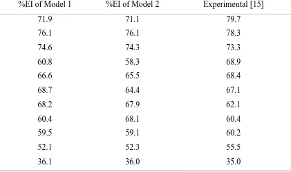
Table 5. Calculated %IE and Experimental of thiophene derivatives

%EI of Model 1 %EI of Model 2 Experimental [15]

71.9 71.1 79.7

76.1 76.1 78.3

74.6 74.3 73.3

60.8 58.3 68.9

66.6 65.5 68.4

68.7 64.4 67.1

68.2 67.9 62.1

60.4 68.1 60.4

59.5 59.1 60.2

52.1 52.3 55.5

Application of the above models to test the predictability by calculating the theoretical inhibition efficiency and compare with the experimental %IE of the compound from the literature are shown in Table 5, the result shows a closer similarity in values between the calculated %IE and experimental %IE , compound 1-6 %IE experimental are higher than the calculated , while 7-11 are favored towards calculated values. This is attributed to the nature of the molecular property [22], as well as the possibility of forming an error during experiments [23]. For model 1and 2 the calculated values are closer but model with less number of descriptors is found to be better.

Figure 1. shows the variation in % IE of calculated and experimental with 5 descriptors

Figure 3. Correlation between experimental and calculated %IE with 5 descriptors

Figure 4. Correlation between experimental and calculated %IE with 2 descriptors

R2 = 0.850 1 Latent Variable RMSEC = 2.9218 RMSECV = 14.8548 RMSEP = 6.692 Calibration Bias = 0 CV Bias = 2.9258 Prediction Bias = -2.7491

35 40 45 50 55 60 65 70 75 80

0 100 200 300 400 500 600 700

Y Measured 1

Q R e s id u a ls ( 7 9 .9 8 % )

Samples/Scores Plot of c & Test,

Q Residuals (79.98%) Calibration Test 95% Confidence Level

Figure 5. Studentized residual by y-measured %IE with 5 descriptors

35 40 45 50 55 60 65 70 75 80

-3 -2.5 -2 -1.5 -1 -0.5 0 0.5 1 1.5 2

Y Measured 1

Y S td n t R e s id u a l 1

Samples/Scores Plot of c & Test,

Y Stdnt Residual 1 Calibration Test Zero

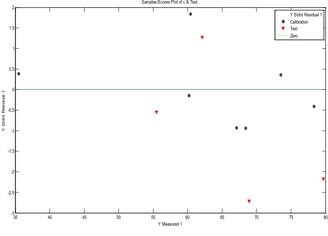
Figure 6. Studentized residual with y-measured %IE with 2 descriptors

3.2. Descriptors interpretation

SpMAD_L is a 2D matrix descriptor explaining the spectral absolute deviation of the Laplace and the correlation of melting point and spartial atom contribution.

MATS4M is the 2D autocorrelation descriptors which define by Moran autocorrealation of lag4 weighted by mass and is showing the effect of branching and non linearity in the compound.

SPMAX3_EA(ed) is an edge adjancy descriptor weighted by edge degree due to the nature and size of the neighboring atom.

RDF10S is the radial distribution function descriptor weighted by 1- state and it relates the shape of the 3D distribution of the atomic mass and the molecular structure of the compound.

R1P is 2D autocorrelation lag1 weighted by polarization. Therefore, higher value of MTS4M, SPMAX3_EA (Ed), RDF10S, R1P and lower value of SpMAD_L descriptors lead to the effective corrosion inhibition of the compound.

4. CONCLUSION

The aim of this work was to develop a QSAR model and predict corrosion inhibition activity of thiophene derivatives. Different descriptors were calculated by Dragon software and selected by interval partial least square (IPLS) method the model built from IPLS in combination with PLS was assessed by internal and external validation and the result shows that the model has prediction power and robustness . The 5 descriptors selected shows that Moran autocorrelation of Lag4 weighted by mass (MATS4M) and Largest eigenvalues n3 of Burden matrix weighted by mass ( SPMAX3_Bh(m)) are the most influential descriptors because of their presence in both the two models. Therefore, this approach can be use to search for more corrosion inhibitors from the properties obtained by dragon software apart from conventional method using quantum chemical calculations by Gaussian software.

We hope that the derived models will be used as precursor in searching more potential corrosion inhibitors from the pool of data prior to experimental evaluation.

ACKNOWLEDGEMENT

I wish to thank the support of computational laboratory, Chemistry Department, Faculty of Science and Research Management Centre (RMC) University Teknologi, Malaysia. I also acknowledge the support given to me by Bayero University Kano, Nigeria and McArthur scholarship Grant for undertaking this program.

References

1. S. G. Zhang, W. Lei, M. Z. Xia, and F. Y. Wang., THEOCHEM, 732 (1–3) ( 2005) 173–182. 2. B. E. A. Rani and B. B. J. Basu. Int J. Corros. (2012) 1–15.

3. C. M. Goulart, A. Esteves-Souza, C. A. Martinez-Huitle, C. J. F. Rodrigues, M. A. M. Maciel, and A. Echevarria, Corros. Sci., 67 (2013) 281–291.

4. Z. El Adnani, M. Mcharfi, M. Sfaira, M. Benzakour, A. T. Benjelloun, and M. Ebn Touhami, Corros. Sci., 68 (2013) 223–230.

5. A. Zarrouk, A. Dafali, B. Hammouti, H. Zarrok, S. Boukhris, and M. Zertoubi, Int. J. Electrochem. Sci. 5 ( 2010) 46–55.

7. E. S. H. El Ashry and S. A. Senior, Corros. Sci., 53 ( 2011) 1025–1034. 8. K. F. Khaled, Corros. Sci., 53 (2011) 3457–3465.

9. I. B. Obot, S. A. Umoren, and E. E. Ebenso, Quantum., 6 ( 2011) 5649–5675.

10.N. O. Eddy, F. E. Awe, C. E. Gimba, N. O. Ibisi, and E. E. Ebenso, Int. J. Electrochem. Sci., 6 (2011) 931–957.

11.M. S. Masoud, M. K. Awad, M. A. Shaker, and M. M. T. El-Tahawy, Corros. Sci., 52 ( 2010) 2387–2396.

12.A. J. Leo and C. Hansch, Perspectives in drug discovery and design, kluwer - Academic Publication , Netherland, (1999).

13.A. Beheshti, E. Pourbasheer, M. Nekoei, and S. Vahdani, Arabian J. Chem, (2012) in press. 14.Z. Xiaobo, Z. Jiewen, M. J. W. Povey, M. Holmes, and M. Hanpin, Anal. Chem. Acta., 667 (1–2)

(2010) 14–3.

15.K. F. Khaled, Int. J. Electrochem. Sci. 7 ( 2012) 1045–1059.

16.A. Golbraikh, M. Shen, Z. Xiao, Y. D. Xiao, K. H. Lee, and A. Tropsha, J. Comput.-Aided Mol. Des.,17 ( 2003) 241–253.

17.R. Toderschini “Author ’ s personal copy,”vol. 4, pp. 129–172, 2009.

18.A. Golbraikh and A. Tropsha, J. Comput.-Aided Mol. Des., 16 (2002) 357–69. 19.X. Zou, J. Zhao, H. Mao, J. Shi, X. Yin, and Y. Li, Appl. Spect., 64 (2010) 786–94. 20.A. Golbraikh and A. Tropsha, J. Mol. Graphics Modell. 20 (2002 269–76.

21.A. F. C. Pereira, M. J. C. Pontes, F. F. G. Neto, S. R. B. Santos, R. K. H. Galvão, and M. C. U. Araújo, Food Res. Int., 41 ( 2008) 341–348.

22.G. Gece, Corros. Sci, 50 (11) ( 2008) 2981–2992.