PestNet : an end-to-end deep learning approach for large-scale multi-class pest detection and classification

White Rose Research Online URL for this paper:

http://eprints.whiterose.ac.uk/150790/

Version: Accepted Version

Article:

Liu, L., Wang, R., Xie, C. et al. (4 more authors) (2019) PestNet : an end-to-end deep

learning approach for large-scale multi-class pest detection and classification. IEEE

Access, 7. pp. 45301-45312.

https://doi.org/10.1109/access.2019.2909522

© 2019 IEEE. Personal use of this material is permitted. Permission from IEEE must be

obtained for all other users, including reprinting/ republishing this material for advertising or

promotional purposes, creating new collective works for resale or redistribution to servers

or lists, or reuse of any copyrighted components of this work in other works. Reproduced

in accordance with the publisher's self-archiving policy.

[email protected]

Reuse

Items deposited in White Rose Research Online are protected by copyright, with all rights reserved unless indicated otherwise. They may be downloaded and/or printed for private study, or other acts as permitted by national copyright laws. The publisher or other rights holders may allow further reproduction and re-use of the full text version. This is indicated by the licence information on the White Rose Research Online record for the item.

Takedown

If you consider content in White Rose Research Online to be in breach of UK law, please notify us by

Date of publication xxxx 00, 0000, date of current version xxxx 00, 0000.

Digital Object Identifier 10.1109/ACCESS.2017.Doi Number

PestNet: An End-to-End Deep Learning

Approach for Large-Scale Multi-Class Pest

Detection and Classification

Liu Liu1,2_{, Rujing Wang}1_{, Chengjun Xie}1,*_{, Po Yang}3,*_{, Senior Member, IEEE, Fangyuan}

Wang1,2_{, Sud Sudirman}3 _{and Wancai Liu}4

1_{Institute of Intelligent Machines, and Hefei Institute of Physical Science, Chinese Academy of Sciences, Hefei, 230031 China} 2_{University of Science and Technology of China, Hefei, 230026 China}

3_{Liverpool John Moores University, Liverpool, L3 3AF United Kingdom} 4_{National Agro-Tech Extension and Service Center, Beijing, 100125 China}

*Corresponding authors: Chengjun Xie (e-mail: [email protected]), Po Yang (e-mail: [email protected])

This work was supported by The National Key Technology R&D Program of China under Grant 2018YFD0200300 and the National Natural Science Foundation of China under grant 31401293, 31671586, 61773360.

ABSTRACT Multi-class pest detection is one of crucial components in pest management involving localization in addition to classification which is much more difficult than generic object detection because of the appearance differences among pest species. This paper proposes a region-based end-to-end approach named PestNet for large-scale multi-class pest detection and classification based on deep learning. PestNet consists of three major parts. Firstly, a novel module Channel-Spatial Attention (CSA) is proposed to be fused into Convolutional Neural Network (CNN) backbone for feature extraction and enhancement. The second one is called Region Proposal Network (RPN) that is adopted for providing region proposals as potential pest positions based on extracted feature maps from images. Position-Sensitive Score Map (PSSM), the third component, is used to replace Fully Connected (FC) layers for pest classification and bounding box regression. Furthermore, we apply Contextual RoI (Contextual Region of Interest) as contextual information of pest features to improve detection accuracy. We evaluate PestNet on our newly collected large-scale pests image dataset, Multi-class Pest Dataset 2018 (MPD2018) captured by our designed task-specific image acquisition equipment, covering more than 80k images with over 580k pests labeled by agricultural experts and categorized in 16 classes. Experimental results show that the proposed PestNet performs well on multi-class pest detection with 75.46% mean Average Precision (mAP), which outperforms the state-of-the-art methods.

INDEX TERMS Channel-Spatial Attention, Convolutional Neural Network, Multi-class Pest Detection, Position-Sensitive Score Map, Region Proposal Network

I. INTRODUCTION

In agriculture field, specialized control of numerous pests has always been a key issue affecting agricultural productivity for decades. Thus, monitoring for the number of pest species is of great significance to eliminate pests without delay to avoid blind use of pesticides which result in unhealthy crops. There are millions of species of pests in the world making pest detection becoming one of the major challenges in agriculture pest management. Previously, pest detection is performed by manual observation which is obviously laborious and error-prone.

With the development of modern computer science, computer vision has become an increasingly and widely used

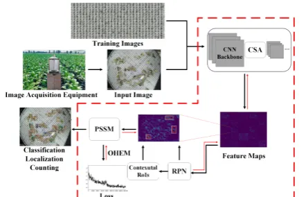
FIGURE 1. Technical pipeline of our PestNet. The components surrounded by red bold dotted box will go through the prior training phase on training images before test phase. The red arrows in this box represent the gradient descent process of the backward propagation stage during training.

FIGURE 2.Sample images of 16 Pest Species in our Work. Note that these sample images are partially taken from images of MPD2018.

by introducing new features, yet paying more attentions on developing novel architectures for large-scale multi-class pest detection task that requires to achieve not only pest recognition but also localization and number counting, which is more helpful for pest monitoring [3,4].

In this context, motivated by the various applications of Convolutional Neural Network (CNN) in deep learning [5-8] and the development of region-based CNN detection techniques in generic objects [9,10], we develop an end-to-end architecture PestNet based on deep learning for multi-class pest detection, whose pipeline is shown in Fig. 1, in which features are extracted and learned from original images automatically without any preprocessing rather than hand-crafted. In order to validate our PestNet, we design an image capture equipment to build our 10-year-term of task-specific dataset Multi-class Pest Dataset 2018 (MPD2018) covering more than 80k images with over 580k pests labeled by agricultural experts and categorized in 16 classes, and some of pests’ examples are shown in Fig. 2. In PestNet, images are firstly input into a CNN backbone for feature extraction and the output is so-called 'feature maps'. In this phase, we propose Channel-Spatial Attention (CSA) module to enhance the channel and spatial information between every two convolutional blocks. Then we apply Region Proposal Network (RPN) to compute region proposals for each position in feature maps. These regions could distinguish between pests and non-pests so they indicate the potential pests’ positions.

The goal of the following step is to predict pests’ categories and fine-tune bounding boxes from region proposals. In generic object detection methods, the feature maps are taken a pooling operation based on the region

proposals for cropping into a fixed size. In PestNet, we augment contextual information named Contextual Regions of Interest (Contextual RoIs) into the region proposals and fuse them together for more accurate prediction. Furthermore, many state-of-the-art CNN methods for detecting generic objects adopt Fully Connected (FC) layer to achieve prediction [11]. But FC might be insensitive to spatial location which is a major limitation leading to worse results. Besides, FC holds large number of parameters causing much more computational cost, which might affect real time performance. In PestNet, to address these issues, a module called Position-Sensitive Score Map (PSSM) is used to replace FC layer, which could compute confidence scores of each position in proposed regions. Moreover, Online Hard Example Mining (OHEM) [12] strategy is used for improving the effectiveness of training. The entire training and test phase could run automatically to achieve pest detection and classification so PestNet is an end-to-end system.

The major contributions of this paper are as follows: 1) A novel end-to-end convolutional neural network based automatic pest detection architecture PestNet is designed and developed for large-scale multi-class pest detection and classification.

2) PestNet is a region-based approach adopting Region Proposal Network (RPN) for providing pest regions and Position-Sensitive Score Map (PSSM) for pest classification and bounding box regression. Furthermore, our method obtains improved pest detection accuracy by integrating a novel feature enhancement module Channel-Spatial Attention (CSA) and considering Contextual Regions of Interest (Contextual RoIs) for accurately classifying the types of pests and qualifying their positions.

3) We build a 10-year-term of large-scale pest dataset Multi-class Pest Dataset 2018 (MPD2018) captured by our designed task-specific image acquisition equipment, covering more than 80k images with over 580k pests labeled by agricultural experts and categorized in 16 classes.

II. RELATED WORK

rotation, scale and translation. To deal with it, employed Scale-invariant feature transform (SIFT) was employed with LOSS algorithm to classify five insects [4]. Meanwhile, compared with previous classifiers such as k-nearest neighbors [18] and linear discriminate analysis (LDA) [19], support vector machine (SVM) was proposed with Haar-like features to classify insects and obtained a better performance than the state-of-the-art methods [20]. In terms of neural network approaches, Artificial Neural Network (ANN) was adopted as well as SVM based on their own designed features [21]. In addition, ANN was also used for categorizing butterfly and other insects [22,23].

Although the aforementioned pest identification methods have achieved great success to some extent, their results rely too much on hand-crafted features selection such as SIFT and Haar. In this case, one potential consequence is that the extracted descriptors show strong similarity to others among pests. i.e. the feature vectors with different species are highly close in feature space because of the relative variability of their texture, color, shape and so on. Furthermore, the processing of designing features is laborious and insufficient to represent all aspects of the insects. As a result, sustainable insect detection methods should rely on greater depth to mine more valuable information and learn features automatically instead of blind low-level feature descriptors.

Another limitation is that few previous works using traditional machine learning methods aim to address multi-class pest detection issue that focuses more on pest localization which is much more difficult than classification. As it is well known, CNN in deep learning has made an obvious breakthrough on computer vision in the recent years for generic object detection [24-26]. Many sorts of algorithms based on CNN have emerged to significantly improve current systems performance for classification as well as object localization [27]. Besides, CNN architecture could also achieve automatic feature extraction. In agricultural area, deep learning has also received widespread attention in the past two years. Among these works, the region-based architectures especially Faster RCNN are the most popular choice to detect generic in-field insects [28,29]. Besides, Single-Shot Detector (SSD) [30] is another common method used in plant disease and pest detection [31]. For pest identification task, ResNet has become a widely used CNN backbone to extract pest features. Therefore, we propose region-based end-to-end approach named PestNet for large-scale multi-class pest detection and classification based on deep learning, which improves performance by the following aspects. Firstly, a novel module Channel-Spatial Attention (CSA) is proposed into CNN based network for feature extraction and enhancement. Secondly, for pest localization, we employ a region proposal method combined with PSSM module generating candidate boxes automatically, in which Contextual RoI (Contextual Region of Interest) as contextual information are augmented. Such this end-to-end method does not require any preprocessing as well as human intervention and could yield state-of-the-art performance.

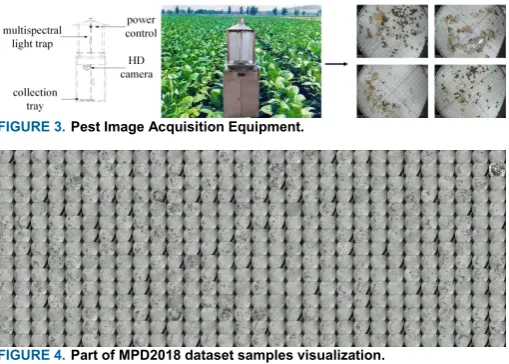
FIGURE 3.Pest Image Acquisition Equipment.

FIGURE 4.Part of MPD2018 dataset samples visualization.

III. MATERIALS AND METHODS

A. MULTI-CLASS PEST DATASET 2018 (MPD2018)

For agriculture pest identification, there exist a few open datasets released such as Butterfly Dataset [32]. However, to our best knowledge, few open datasets suitable for multi-class pest detection task are released while our purpose is to detect different kinds of pests simultaneously in one image. As a result, we build a dataset for our large-scale multi-class pest detection task. Specifically, the pest image acquisition equipment designed for capturing images of multi-class pests in our dataset is shown in Fig. 3. In this device, the multispectral light trap could emit light for attracting multi-class pests, in which the wavelengths could vary with time according to habits of pests in the day to ensure different types of pests could be captured. Then these attracted pests would be stunned by the screen and fall into the pest collection tray on the bottom. At the same time, the HD camera in the tray above is set to take pictures periodically at 15 second intervals. After being photographed, the pests would be swept away from the pest collection tray immediately to avoid accumulation and overlapping. The captured images are stored in JPG format at 2592 1944

resolution. Hereafter, each pest in images are annotated by agricultural experts with labels and bounding boxes. Finally, 88,670 images containing 582,170 pest objects categorized in 16 classes are captured. Our newly built dataset is named Multi-class Pest Dataset 2018 (MPD2018) and part of examples are visualized in Fig. 4.

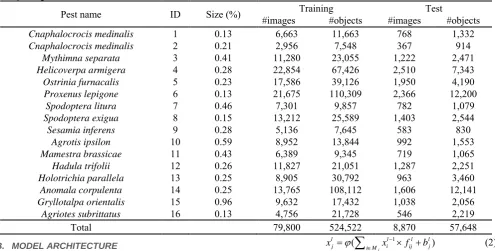
Table 1. Statistics on Two Subsets in MPD2018. The dataset is divided into training and test subsets. For each class, the number of images (containing at least one pest the class) and that of objects are shown in columns. ‘Size’ represents the percentage of the area of object in the whole image. Note that because single image may contain objects of several classes, the totals shown in the ‘#images’ columns are not simply the sum of the corresponding columns.

Pest name ID Size (%) _#images Training _{#objects #images} Test _#objects

Cnaphalocrocis medinalis 1 0.13 6,663 11,663 768 1,332

Cnaphalocrocis medinalis 2 0.21 2,956 7,548 367 914

Mythimna separata 3 0.41 11,280 23,055 1,222 2,471

Helicoverpa armigera 4 0.28 22,854 67,426 2,510 7,343

Ostrinia furnacalis 5 0.23 17,586 39,126 1,950 4,190

Proxenus lepigone 6 0.13 21,675 110,309 2,366 12,200

Spodoptera litura 7 0.46 7,301 9,857 782 1,079

Spodoptera exigua 8 0.15 13,212 25,589 1,403 2,544

Sesamia inferens 9 0.28 5,136 7,645 583 830

Agrotis ipsilon 10 0.59 8,952 13,844 992 1,553

Mamestra brassicae 11 0.43 6,389 9,345 719 1,065

Hadula trifolii 12 0.26 11,827 21,051 1,287 2,251

Holotrichia parallela 13 0.25 8,905 30,792 963 3,460

Anomala corpulenta 14 0.25 13,765 108,112 1,606 12,141

Gryllotalpa orientalis 15 0.96 9,632 17,432 1,038 2,056

Agriotes subrittatus 16 0.13 4,756 21,728 546 2,219

Total 79,800 524,522 8,870 57,648

B. MODEL ARCHITECTURE

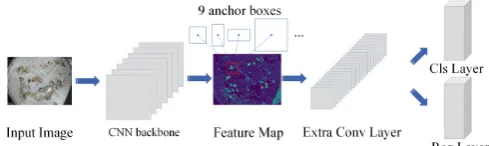
Our PestNet consists of three stages: pest feature extraction, pest regions search and pest prediction. In PestNet, the input image is firstly fed into a CNN backbone to extract feature maps, where CSA module is proposed for feature enhancement. Then we fuse RPN and PSSM for providing pest regions and pest prediction respectively. During the prediction phase, Contextual RoIs are presented as contextual information to improve detection accuracy.

1) CONVOLUTIONAL NEURAL NETWORK (CNN)

Conventional computer vision employed hand-crafted features to describe the images. Instead, we adopt CNN for automatic feature extraction which is basically composed of 3 parts: convolutional layer, activation function, and pooling layer.

Convolutional Layer: Standard convolutional layer takes a set of filters (also called kernel) as a filterbank to the input and the output feature map in each subsequent layer could be regarded as abstract transformations of image. Take a size of

1 1 1

l l l

W  H  C feature map and a filterbank within Cl filters at size of l l l 1

f f C in layer l1 for example,

augmenting the other two hyper-parameters padding l p and

stride l

s , the output feature map in layer l is at size of

l l l

W H C :

( ,l l) ( l 1, l 1) 2 l l 1 l

W H p f

W H

s

 

   

_  _

  (1)

where    denotes floor operation. Note that the number of

filters must be equal to that of input feature map. More specifically:

1

( )

j

l l l l

j i M i ij j

x 



where i and j are indexes of input and output feature maps at range of _Wl_Hl and _Wl1_Hl1 respectively.

j

M here indicates the receptive field of filter and l

j

b is bias term. Activation Function: In the equation (2), ( ) is called activation function applied to achieve element-wise non-linearity in deep learning, which contains many types such as sigmoid, Rectified Linear Units (ReLU) [33]. In our method, we utilize ReLU as activation function for faster training because of larger gradient in (0, ) :

( ) max(0, )x x

  (3) Pooling Layer: In CNN, pooling layer is usually applied for feature dimension reduction. Besides, spatial translational invariance is another benefit of pooling layer. Among different pooling layer methods, max-pooling layer is selected in PestNet which applies local pooling by preserving maximum of receptive field and discarding other values. 2) CHANNEL-SPATIAL ATTENTION (CSA)

large background noises as shown in Fig. 5 (left part). This is because that the convolutional operation owns a well-known defect of limited receptive field. Thus, it is possible to obtain a higher detection performance by applying global spatial attention to filter the feature maps.

Inspired by these two observations, we propose a novel module Channel-Spatial Attention (CSA) for weighting channel and spatial information on output from each CNN block to enhance the representational power of feature maps. Fig. 5 shows an intuitive framework of our CSA module in the backbone that consists of two parts. In the first part of Channel Attention module (the upper part), the 3D feature map with shape of W H C extracted by CNN block is input into an extra global pooling layer that takes average pooling from the whole feature maps in each channel to generate a lower dimensional (1D) feature vector, in which the averaged value represents the global feature for each channel. Then, we apply a group of convolutional layers with non-linear activation ReLU following. This 1D feature vector is mapped into (0,1) area by adopting Sigmoid function and the output with shape of 1 1 C is so-called channel attention factor. Thus, the output of Channel Attention module is the broadcast element-wise product of the original input 3D feature map and the 1D channel attention factor. In this way, the input 3D feature map is activated in channel level.

FIGURE 5.Channel-Spatial Attention architecture.

The lower part in Fig. 5 is Spatial Attention module, whose operations are similar with Channel Attention module. In this part, the input 3D feature map (W H C) is fed into another convolutional layer with 1 1 kernel and only 1 filter to achieve global convolution. The output is a 2D feature map with shape of W H 1, so each value

could be a global feature for spatial level. To extract the global spatial information, we adopt an extra convolution operation with a large kernel size (e.g. 7 7 )and to zoom out the feature map into W/ 2H/ 2 1 shape. Next, a corresponding deconvolution operation is applied to generate the spatial attention factor (W H 1) and the

input 3D feature map is multiplied by the spatial attention factor in each spatial position so the feature map is activated in spatial level. Finally, the output of CSA is the sum of two activated feature maps.

3) REGION PROPOSAL NETWORK (RPN)

Our PestNet is a region-based CNN method so we adopt RPN module to search potential regions of object followed by CNN backbone. As RPN holds its own objectness scores and bounding box regression layer, it could effectively

provide regions automatically. In contrast to other relevant methods e.g. selective search [34] and edge boxes [35] which spends much time on thousands of regions, RPN could reduce a large number of proposal regions when ensuring the quality by introducing various anchor boxes for box regression reference.

FIGURE 6.Region Proposal Network architecture.

Fig. 6 shows an intuitive framework of RPN module in training phase. As it can be seen, the feature map extracted by base CNN is input into an extra convolutional layer which takes sliding windows to generate a lower dimensional region feature. For every sliding window in standard RPN module, there are 9 rectangular region boxes totally with 3 kinds of scales _{{128 ,256 ,512 }}2 2 2 _{and ratios}

{1:1,1: 2,2 :1}. Here for detecting pests with tiny sizes in MPD2018, we compute our own scales _{{64 ,128 ,256 }}2 2 2

specifically which ensures effective receptive field on input images for finding tiny pests. These boxes are also called anchors and could be referenced for coarse-tuning in next two sibling regression layers, which are fully connected. The two layers are called box classification and regression layers respectively employed for bounding boxes revision and the output is 2 9 scores and 4 9 coordinates based on 9 reference boxes, describing class scores for background and non-background regions and bounding boxes (x_min,y_min,x_max,y_max). Finally, RPN provides large number of region proposals also called Region of Interest (RoI) for next processing.

4) POSITION-SENSITIVE SCORE MAP (PSSM)

The following step is to classify the categories and fine-tune RoIs. In order to ensure translational invariance of RoIs, we adopt position-sensitive score maps (PSSM) to encode position information. As it is shown in Fig. 7, an extra convolutional layer is firstly extended after CNN backbone to produce a _{7 (}2 ₁₎

C channels score map

bounding box fine-tuning by augmenting an extra

2

4 7 ( C1) channels convolutional layer and it could produce 4(C1) channels in a similar way. Therefore, in PSSM method, the two score maps are sensitive to positions of region proposals because various channels indicate different positions.

FIGURE 7.Position-Sensitive Score Map architecture.

For predicting categories as well as bounding boxes, we employ softmax regression which is an expansion of logistic regression [36]. Besides, we define a threshold to filter most of boxes which hold low scores and non-maximum suppression (NMS) [37] is also applied to retain regions with locally maximal scores, in which Intersection-over-Union (IoU) is adopted as metrics to eliminate most of overlapping boxes, in which:

( , ) A B IoU A B

A B

 

 (4)

5) PEST CONTEXTUAL ROIS

To enhance the RoI information during box regression phase in PSSM, we take full advantage of contextual information of RoIs. The motivation is that the input of RoI pooling operation is derived from the original region proposals that are outputted from RPN, in which the information of pest might not be completely covered. In this case, some supportive contextual information that could help bounding boxes fine-tuning would lose leading to unsatisfied regression results. Thus, as shown in Fig. 8, we augment extra contextual information called Contextual RoI, which are expansion of 1.5 times larger than original RoIs. Then we append another RoI pooling on these extra contextual RoIs and fuse the two results. Through this way, the contextual information could be added into RoIs and fully utilized as extra auxiliary information for better results.

C. MODEL OPTIMIZATION

1) LOSS FUNCTION AND OPTIMIZER

Loss function is the criterion for training process. Our loss function is defined as the sum of the cross-entropy loss and the box regression loss:

( , ) cls( )c [ 0] reg( , ) L s t L s c L t t

 

   (5) where s_c denotes the predicted score class c while t and t denote { , , , }t t t t_{x y w h} of bounding boxes. [ c 0] indicates that we only consider the boxes of

non-background (the box is non-background if

c



0

function contains two parts for classification loss Lcls and

bounding box regression loss Lreg, in which:

( ) log( )

cls c c

L s   s (6) and

1 ( , , , )

( , ) ( )

reg _{i x y w h} L i i

L t t 



where:

2

1

0.5 if x <1 ( )

0.5 otherwise

L

x smooth x

x



  _

 (8)

In terms of optimizer, the momentum SGD [38] is chosen as our optimizer with momentum 0.9, which updates parameters based on one sample at each iteration. This optimizer could partly keep the update gradient at previous iteration and fine-tune the final gradient. In order to avoid over-fitting problem, we utilize dropout method [39] as well as early-stopping strategy [40] to select the best training iteration. As to learning rate policy, 'step' strategy is applied in gradient descent, in which we initialize learning rate to 0.001 and the learning rate will be divided by 10 per 50000 iterations. In addition, mini-batch size is set to 1 and the number of region proposals of every training example is at least 256.

FIGURE 8.Process of Contextual RoI.

2) ONLINE HARD EXAMPLE MINING (OHEM)

In order to achieve efficient training in our task, we append Online Hard Example Mining (OHEM) [12] as a training example selection strategy to enhance our learning consequent during training phase. OHEM mines hard regions for more effective backward propagation. In OHEM approach, we compute the loss of all N region proposals for one image in forward propagation. Then NMS method is applied to select B regions that have highest loss because highly overlapping regions might result in loss double counting problem. Therefore, in backward propagation, the model parameters are updated only based on these selected regions while we set the gradients of other N-B regions to 0.

IV. EXPERIMENTS

A. EXPERIMENTAL SETTINGS

data with original training images for doubling data volume to enlarge data amount for learning more invariant features. Therefore, we could obtain more examples for training to avoid over-fitting problem. In the aspect of experiments design, we train four CNN backbones with Faster RCNN [11] that contains RPN and fully connected network (FC) as the baseline in our experiments, which is one of the state-of-the-art architectures. Furthermore, we compare the performance of our PestNet with a state-of-the-art one-stage object detection method SSD [42] that is also a common choice in pest detection task. In addition, we adopt transfer learning [41] method to use CNN backbones pre-trained on ImageNet dataset as our model initial parameters.

B. CNN BACKBONES

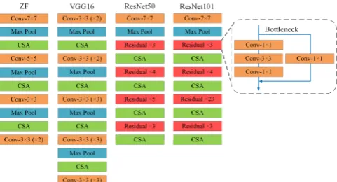
In our experiments, we are going to consider four CNN architectures of different complexity as prior CNN backbones with our CSA module for feature extraction which are ZF [24], VGG16 [25], ResNet50 and ResNet101 [26] whose details are shown in Fig. 9, where ZF and VGG16 are shallow CNNs while ResNet50 and ResNet101 are deep CNNs. In deep networks that contain residual blocks, we use bottleneck [43] to reduce computational cost by adopting extra convolution operation.

FIGURE 9.CNN backbones Details in PestNet. The integers followed by 'Conv' denote the kernel sizes.

C. EVLUATION METRICS

In order to accurately validate our model, mean Average Precision (mAP) is used as a major evaluation metrics that takes mean of Average Precision (AP) value among classes. AP value is defined as the area under Precision-Recall (PR) curve:

1 0

( ) Prcision(c) Recall(c)

C

AP c 



where c denotes the class, Precision-Recall is calculated by: # ( )

( )

# ( ) # ( ) TP c Precision c

TP c FP c



 (10)

# ( ) ( )

# ( ) # ( ) TP c Recall c

TP c FN c



 (11)

in which

TP

FP

FN

while higher Recall indicates the lower misdetection rate. So, the mAP could be obtained by taking mean:

1 _{( )}

c C

mAP AP c

C 





V. RESULTS AND DISCUSSION

A. TRAINING LOSS ANALYSIS

Training iteration is one of the major hyper-parameters in PestNet because proper iteration could assist to avoid overfitting problem. As it can be seen in Fig. 10 illustrating the training loss curves, with the iteration increasing, the training losses could keep dropping at approximately first 20k iterations, which indicates that our models could learn to detect the pests’ features well at the beginning of training phase. When networks continue iterating, the decline of training loss turns to be slower. During the iteration of 100k to 120k, the models become to achieve convergence. Therefore, we choose 120k as the best training iteration parameter in our experiments for training our model. It also could be observed in Fig. 10 that deep CNN architectures could obtain lower loss than the shallow network ZF. Furthermore, the training losses of ResNet50 as well as ResNet101 are more stable while there are large fluctuations in the curves of ZF and VGG16 networks.

FIGURE 10. Training loss on four different architectures grouped into ‘shallow’ models and ‘deep’ models based on their network’s depth. Training loss is calculated by summing loss and bounding box regression loss.

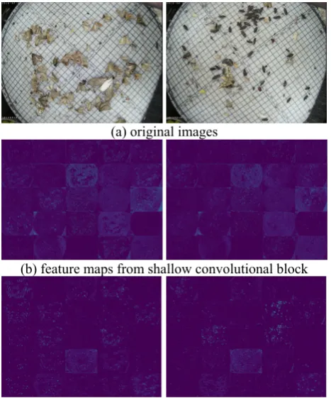
B. FEATURE VISUALIZATION

In order to prove the learning capacity of PestNet, part of feature maps outputted from 2 middle blocks in ResNet101 are visualized in Fig. 11. As it is shown, lots of feature maps in shallow convolutional block are influenced by grid lines of background while only a small part of those could filter the objects well. With the layer going deeper, points of pests are activated better and become clearer, which could neglect irrelevant content and extract valuable features of the pests. Meanwhile, features maps in deep convolutional block could separate the objects and the activation values of points are much brighter than background in feature maps. Among these figures, it is obvious that PestNet could progressively learn the pests' features using deep CNN.

C. PRECISION-RECALL ANALYSIS

precision could keep a high value in a small range of recall. Besides, PestNet using different backbone CNNs could obtain a larger precision and recall compared with Faster RCNN and SSD so PestNet could effectively reduce false positives rate as well as misdetections rate. Specifically, class #2 is relatively difficult to detect because the PR curve for this class is further away from the point (1,1). In addition, there is a significant decline in PR curves of class #9 and #16, which indicates that more false positives are detected leading to lower precision. Furthermore, among these illustrated PR curves, PestNet performs best on class #16 with the highest integral of the PR curve, which means that a high precision in addition to recall could be obtained at same time.

(a) original images

(b) feature maps from shallow convolutional block

(c) feature maps from deep convolutional block FIGURE 11. Feature maps generated by PestNet using ResNet101 as CNN backbone. Each box shows its corresponding filter response. Note that only the first 25 feature maps are visualized because of space limitation and the sizes of feature maps are shrinking from top to down and the figure shows same size for best view.

(a) mean PR Curve among all the classes

(b) PR Curve for class 2 (c) PR Curve class 3

(d) PR Curve for class 9 (e) PR Curve class 16 FIGURE 12.Mean Precision-Recall curve among all the classes and part of curves for some classes with different methods and backbone CNNs. Note that only PR curves of only 4 classes are shown here due to space limitation.

D. MULTI-CLASS PEST DETECTION RESULTS

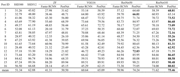
Table 2 presents the final multi-class pest detection results on test set of MPD2018 using PestNet, SSD and Faster RCNN with various CNN backbones. As it can be seen, SSD seems to be an unsatisfied approach in pest detection task, which could only obtain 51.34% and 62.88% mAP on 16 pest categories. This phenomenon could be attributed to the limitations of one-stage detector such as inadequate feature extraction. Compared with other two-stage pest detection approach, it is clear that PestNet architecture could significantly outperform Faster RCNN using ZF network on almost all classes, leading to around 9.19% improvement. Similarly, the homologous advance appears in the two deep networks ResNet50 and ResNet101, which improving 3.28% and 4.84% mAP respectively. This gain is largely due to our CSA’s ability to activate the channel and spatial information more rather than simple fully connected layer for pest recognition, which is helpful to sufficiently learn the features of pests in global channel and spatial level. Furthermore, Faster RCNN and PestNet might obtain lower mAP on shallow CNN backbones because of lower quality of feature maps in shallow models. Another observation derived in Table 2 is that although the best performance occurs in PestNet using ResNet101 which achieves detection precision with 75.46% mAP, there does not exist a large difference between PestNet with ResNet101 and that with ResNet50. This might be explained by Fig. 10 where training losses of these two models are showed to be close in training phase, implying that more depth of network could be less significant in improving performance when model owns enough depth.

them by comparing Table 2 and Table 1. Furthermore, the number of training examples would also affect model performance, where classes #4, #5 and #14 who hold large training volumes are detected with more than 70% AP even they are very tiny object. Meanwhile, PestNet could dramatically improve detection accuracy of these 'difficult' pest species while maintain a strong performance for the 'easy' categories. However, in shallow convolutional network (ZF, VGG16), PestNet might not get improvement in class #12 due to the limited number of training samples (6389 samples for class #11). But this case does not occur in deep convolutional networks because of more depth leading to efficient learning so deep CNN ResNet50 as well as ResNet101 could slightly overcome the sample limitation problem with a great improvement.

E. REAL-TIME ANALYSIS

Real-time performance investigation also shows a dramatic improvement on both training and test phase as PestNet could detect and classify the pests faster (Table 3) than Faster RCNN. For Faster RCNN, this is due to the replacement of PSSM module with FC layer, in which fully convolutional layer in PSSM module holds much less calculation than FC layer. This phenomenon is more pronounced in deep networks rather than shallow networks, in which the test speed of more than 0.6 seconds per image might result in much slow system response. Therefore, PestNet could greatly reduce the impact of this drawback in deep networks with the test speed of 0.441s per image. In

terms of one-stage detector, SSD is the fastest pest detection approach among these methods due to the designed structure of one-stage detector which adopts fully convolutional layers for predicting pests’ boxes and their corresponding categories instead of using RPN. However, SSD could not detect and classify pests in MPD2018 with a passable mAP so it might not be applied in practical pest monitoring.

F. DISCUSSSION AND ANALYSIS

Part of the final results are visualized in Fig. 13 and 14. As it can be seen, PestNet could achieve multi-class pest detection well under both simple and complex scenarios, despite some intractable challenges such as noisy image and tiny objects. Meanwhile, Fig. 13 (c) illustrates that some of occluded pests are also localized and categorized in our model. In pest detection results under complicated scenario, occlusion and dense pest distribution might be the major challenge influencing the detection performance of PestNet. Even though, our method could still localize them well with a few tiny pests missing because our Contextual RoIs augmentation considering more contextual information of each pest region that is helpful to filter pests’ features. Another difficulty of complex scenario is that non-target insects influence, including beneficial insects and less harmful pests that do not need monitoring. PestNet could also distinguish pests from these non-target insects because of proposed CSA module for adequate feature learning.

Table 2. Multi-class Pests Detection Results AP value (%)

Table 3. Training and test time spent per image on different models (s/image)

SSD300 SSD512 ZF VGG16 ResNet50 ResNet101

Faster RCNN PestNet Faster RCNN PestNet Faster RCNN PestNet Faster RCNN PestNet training 0.077 0.084 0.327 0.288 0.517 0.452 0.686 0.573 0.712 0.618

test 0.031 0.043 0.108 0.101 0.185 0.177 0.616 0.413 0.636 0.441

Pest ID SSD300 SSD512 ZF VGG16 ResNet50 ResNet101

Faster RCNN PestNet Faster RCNN PestNet Faster RCNN PestNet Faster RCNN PestNet

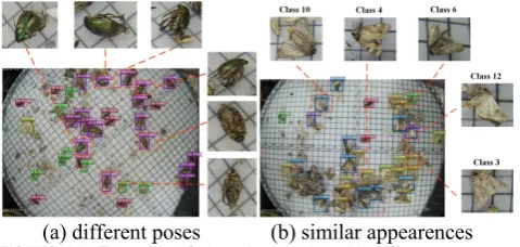
Specifically, some typical examples are shown in Fig. 14, in which pests from the same class but under large different poses, such as frontal side and back side, could also be found precisely. Besides, PestNet could also solve the problem that similar pest identification in different classes (Fig. 14 (b)).

VI. CONCLUTION

This paper proposed a novel end-to-end automatic pest detection network PestNet, which successfully achieves large-scale multi-class pest detection. Our PestNet could realize the automatic extraction of higher quality features by our proposed CSA module that is a novel feature enhancement module. Furthermore, compared to many common object detection methods, we adopted PSSM instead of FC for computational cost reduction in pest classification and box regression process. Besides, contextual RoIs was also considered as contextual information in PestNet to further improve detection performance. Under our enriched dataset MPD2018, PestNet have achieved a higher mAP (75.46%) among 16 classes of pests than the state-of-the-art methods.

(a) One class pest detection

(b) Multi-class pest detection under simple scenario

(c) Multi-class pest detection under complex scenario FIGURE 13. Examples of pest detection results demonstration. These results are outputted by PestNet model based on ResNet101. The scenarios of input images from top to bottom are more and more complicated. Note that some certain insects are not localized and classified here because they are some kind of beneficial insects rather than 16 types of pests in our MPD2018.

(a) different poses (b) similar appearences FIGURE 14. Examples of detection results with different poses and similar appearances.

REFERENCES

[1] J. Wang, C. Lin, L. Ji and A. Liang, “A new automatic identification system of insect images at the order level,” Knowledge-Based Systems, vol. 33, pp.102-110, 2012.

[2] P. Fedor, I. Malenovský, J. Va hara, W. Sierka and J. Havel, “Thrips (Thysanoptera) identification using artificial neural networks,” Bulletin of entomological research, vol. 98, no. 5,

pp.437-447, 2008.

[3] M. E. Nilsback and A. Zisserman, “Automated flower classification over a large number of classes,” in Computer Vision, Graphics & Image Processing, 2008. ICVGIP'08. Sixth Indian Conference on,

2008, pp. 722-729.

[4] L. O. Solis-Sánchez, R. Castañeda-Miranda, J. J. García-Escalante, I. Torres-Pacheco, R. G. Guevara-González, C. L. Castañeda-Miranda and P. D. Alaniz-Lumbreras, “Scale invariant feature approach for insect monitoring,” Computers and electronics in agriculture, vol. 75,

no. 1, pp. 92-99, 2011.

[5] Z. Wang et al., "Efficient rail area detection using convolutional

neural network," IEEE Access., to be published. DOI:

10.1109/ACCESS.2018.2883704.

[6] C. Wu et al., "A Greedy Deep Learning Method for Medical Disease

Analysis," IEEE Access., vol. 6, pp. 20021-20030, 2018.

[7] G. Liang et al., "Combining Convolutional Neural Network With

Recursive Neural Network for Blood Cell Image Classification,"

IEEE Access., vol. 6, pp. 36188-36197, 2018.

[8] D. Hu et al., "A novel image steganography method via deep

convolutional generative adversarial networks," IEEE Access., vol. 6,

pp. 38303-38314, 2018.

[9] R. Girshick. (2015, Apr). Fast r-cnn. arXiv. [online]. Available:

https://arxiv.org/abs/1504.08083.

[10] J. Dai, Y. Li, K. He and J. Sun, “R-fcn: Object detection via region-based fully convolutional networks,” in Advances in neural information processing systems, 2016, pp. 379-387.

[11] S. Ren, K. He, R. Girshick and J. Sun, “Faster r-cnn: Towards real-time object detection with region proposal networks,” IEEE transactions on pattern analysis and machine intelligence, vol. 39,

no. 6, pp. 1137-1149, 2017.

[12] A. Shrivastava, A. Gupta and R. Girshick, “Training region-based object detectors with online hard example mining,” in Proceedings of the IEEE Conference on Computer Vision and Pattern Recognition,

2016, pp. 761-769.

[13] X. Zhang et al., "Identification of Maize Leaf Diseases Using

Improved Deep Convolutional Neural Networks," IEEE Access., vol.

6, pp. 30370-30377, 2018.

[14] C. Xie, R. Wang, J. Zhang, P. Chen, W. Dong, R. Li, T. Chen and H. Chen, “Multi-level learning features for automatic classification of field crop pests,” Computers and Electronics in Agriculture., vol.

152, pp. 233–241, 2018.

[15] I. Y. Zayas and P. W. Flinn, “Detection of Insects in Bulkwheat Samples with Machine Vision,” Transactions of the ASAE, vol. 41,

no. 3, pp. 883, 1998.

[16] P. J. D. Weeks, M. A. O'Neill, K. J. Gaston and I. D. Gauld, “Species–identification of wasps using principal component associative memories,” Image and Vision Computing, vol. 17, no. 12,

pp. 861-866, 1999.

[17] J. Cho, J. Choi, M. Qiao, C. W. Ji, H. Y. Kim, K. B. Uhm and T. S. Chon, “Automatic identification of whiteflies, aphids and thrips in greenhouse based on image analysis,” Red, vol. 346, no. 246, pp. 244,

2007.

[18] C. Wen, D. E. Guyer and W. Li, “Local feature-based identification and classification for orchard,” insects. Biosystems engineering, vol.

104, no. 3, pp. 299-307, 2009.

[19] X. Li, S. Huang, M. Zhou and G. Geng, “KNN-spectral regression LDA for insect recognition,” in Information Science and Engineering (ICISE), 2009 1st International Conference on, 2009, pp. 1315-1318.

[20] N. Larios, B. Soran, L. G. Shapiro, G. Martinez-Munoz, J. Lin and T. G. Dietterich, “Haar random forest features and SVM spatial matching kernel for stonefly species identification,” in Pattern Recognition (ICPR), 2010 20th International Conference on, 2010,

pp. 2624-2627.

[21] J. Wang, C. Lin, L. Ji and A. Liang, “A new automatic identification system of insect images at the order level,” Knowledge-Based Systems, vol. 33, pp. 102-110, 2012.

[23] Y. Kaya and L. Kayci, “Application of artificial neural network for automatic detection of butterfly species using color and texture features,” The visual computer, vol. 30, no. 1, pp.71-79, 2014.

[24] M. D. Zeiler and R. Fergus, “Visualizing and understanding convolutional networks,” in European conference on computer vision, 2014, pp. 818-833.

[25] K. Simonyan and A. Zisserman. (2015, Apr). Very deep convolutional networks for large-scale image recognition. arXiv. [online]. Available: https://arxiv.org/abs/1409.1556

[26] K. He, X. Zhang, S. Ren and J. Sun, “Deep residual learning for image recognition,” in Proceedings of the IEEE conference on computer vision and pattern recognition, 2016, pp. 770-778.

[27] R. Girshick, J. Donahue, T. Darrell and J. Malik, “Rich feature hierarchies for accurate object detection and semantic segmentation,” in Proceedings of the IEEE conference on computer vision and pattern recognition, 2014, pp. 580-587.

[28] Y. Shen, H. Zhou, J. Li, F. Jian and D. S. Jayas, (2018). “Detection of stored-grain insects using deep learning,” Computers and Electronics in Agriculture, vol. 145, pp. 319-325, 2018.

[29] D. Xia, P. Chen, B. Wang, J. Zhang and C. Xie, “Insect detection and classification based on an improved convolutional neural network,”

Sensors, vol. 18, no. 12, pp. 4169, 2018.

[30] F. Alvaro, Y. Sook, K. Sang and P. Dong, “A robust deep-learning-based detector for real-time tomato plant diseases and pests recognition,” Sensors, vol. 17, no. 9, pp. 2022, 2017.

[31] X. Cheng, Y. Zhang, Y. Chen, Y. Wu and Y. Yue, “Pest identification via deep residual learning in complex background,”

Computers and Electronics in Agriculture, vol. 141, pp. 351-356,

2017.

[32] B. Xiao, J. F. Ma and J. T. Cui, “Combined blur, translation, scale and rotation invariant image recognition by Radon and pseudo-Fourier–Mellin transforms,” Pattern Recognition, vol. 45, no. 1,

pp.314-321, 2012.

[33] A. Krizhevsky, I. Sutskever and G.E. Hinton, (2012). “Imagenet classification with deep convolutional neural networks,” in Advances in neural information processing systems, 2012, pp. 1097-1105.

[34] J.R. Uijlings, K.E. Van De Sande, T. Gevers and A.W. Smeulders, “Selective search for object recognition,” International journal of computer vision, vol. 104, no. 2, pp. 154-171, 2013.

[35] C.L. Zitnick and P. Dollár, “Edge boxes: Locating object proposals from edges,” in European conference on computer vision, 2014, pp.

391-405

[36] F. E. Harrell, “Ordinal logistic regression,” in Regression modeling strategies, 2001, pp. 331-343.

[37] A. Neubeck, and L. Van Gool, “Efficient non-maximum suppression,” in Pattern Recognition, 2006. ICPR 2006. 18th International Conference on, 2006, vol. 3, pp. 850-855.

[38] L. Bottou, “Stochastic gradient descent tricks,” in Neural networks: Tricks of the trade, 2012, pp. 421-436.

[39] N. Srivastava, G. Hinton, A. Krizhevsky, I. Sutskever and R. Salakhutdinov, “Dropout: A simple way to prevent neural networks from overfitting,” The Journal of Machine Learning Research, vol.

15, no. 1, pp.1929-1958, 2014.

[40] R. Caruana, S. Lawrence and C. L. Giles, “Overfitting in neural nets: Backpropagation, conjugate gradient, and early stopping,” in

Advances in neural information processing systems, 2001, pp.

402-408.

[41] Y. Bengio, “Deep learning of representations for unsupervised and transfer learning,” in Proceedings of ICML Workshop on Unsupervised and Transfer Learning, 2012, pp. 17-36.

[42] W. Liu et al., “SSD: Single Shot MultiBox Detector,” in European Conference on Computer Vision, 2016.

[43] V. Sze, Y. Chen, T. Yang and J. Emer, “Efficient processing of deep neural networks: A tutorial and survey,” Proceedings of the IEEE,