Applications
.
White Rose Research Online URL for this paper:
http://eprints.whiterose.ac.uk/127176/
Version: Published Version
Article:
Bale, Simon Jonathan, Deshpande, Pratik Dilip, Hough, Mark et al. (2 more authors)
(2018) High-Q Tuneable 10-GHz Bragg Resonator for Oscillator Applications. IEEE
Transaction of Ultrasonics Ferroelectrics and Frequency Control. pp. 1-11. ISSN
0885-3010
https://doi.org/10.1109/TUFFC.2017.2782567
eprints@whiterose.ac.uk https://eprints.whiterose.ac.uk/
Reuse
This article is distributed under the terms of the Creative Commons Attribution (CC BY) licence. This licence allows you to distribute, remix, tweak, and build upon the work, even commercially, as long as you credit the authors for the original work. More information and the full terms of the licence here:
https://creativecommons.org/licenses/
Takedown
If you consider content in White Rose Research Online to be in breach of UK law, please notify us by
High-Q Tuneable 10-GHz Bragg Resonator
for Oscillator Applications
Simon J. Bale ,
Member, IEEE
, Pratik D. Deshpande, Mark Hough, Stuart J. Porter,
Member, IEEE
,
and Jeremy K. A. Everard ,
Member, IEEE
Abstract— This paper describes the design, simulation, and measurement of a tuneable 9.365-GHz aperiodic Bragg resonator. The resonator utilizes an aperiodic arrangement of non (λ/4) low-loss alumina plates (Er=9.75, loss tangent of≈1×10⁻⁵ to
2×10⁻⁵) mounted in a cylindrical metal waveguide. Tuning is
achieved by varying the length of the center section of the cavity. A multi-element bellows/probe assembly is presented. A tuning range of 130 MHz (1.39%) is demonstrated. The insertion loss S21varies from−2.84 to−12.03 dB while the unloaded Q varies from 43 788 to 122 550 over this tuning range. At 10 of the 13 measurement points, the unloaded Q exceeds 1 00 000, and the insertion loss is above −7 dB. Two modeling techniques are discussed; these include a simple ABCD circuit model for rapid simulation and optimization and a 2.5-D field solver, which is used to plot the field distribution inside the cavity.
Index Terms— Bragg resonators, dielectric resonators (DRs), low-noise oscillators, tuneable resonators.
I. INTRODUCTION
T
UNEABLE oscillators are a fundamental element in almost all communication and measurement systems. In these systems, high-Q resonators are required for low phase noise signal generation. This is because in an oscillator the phase slope of the resonator (group delay and Q) causes any internal phase fluctuations, within the bandwidth of the resonator, to be transformed into frequency fluctuations and phase noise.At microwave frequencies, the tuning range and quality factor of conventional resonator structures, such as dielectric resonators (DRs) or yttrium–iron–garnet (YIG) spheres, are limited. The maximum unloaded quality factor attainable from a DR is defined by the loss tangent (tan δ) of the dielectric material as well as the losses introduced by the shield used to enclose the resonator. Modern DRs operating in the TE01δ mode are capable of providing Q-factor of between 10 000 and 30 000 at 10 GHz [1]. At higher frequencies, the dimensions of the dielectric puck can become small if it is operated in a TE or TM hybrid mode, and alternatively, a whispering gallery mode can be used where the field energy is confined to the
Manuscript received June 15, 2015; accepted December 4, 2017. Date of publication December 11, 2017; date of current version January 26, 2018. This work was supported in part by EPSRC project EP/K040820/1 and in part by Selex ES Ltd (now Leonardo MW Ltd). (Corresponding author: Simon J. Bale.)
S. J. Bale, M. Hough, S. J. Porter, and J. K. A. Everard are with the Depart-ment of Electronic Engineering, University of York, Heslington, York YO10 5DD, U.K. (e-mail: simon.bale.@.york.ac.uk; jeremy.everard.@.york.ac.uk;
stuart.porter.@.york.ac.uk; mark.hough.@.york.ac.uk).
P. D. Deshpande is with Viper RF, Newton Aycliffe DL5 6ZE, U.K. (e-mail: pratik.deshpande.@.viper-rf.com).
Digital Object Identifier 10.1109/TUFFC.2017.2782567
outer edge of a ring of dielectric material [2]. The quality factor is then almost entirely defined by the loss tangent of the dielectric and is relatively insensitive to any conducting material boundaries.
Mechanical tuning of a DR can be achieved by perturbing the magnetic field distribution around the resonator by moving a metallic object close to the dielectric material. A tuning range of up to 10% can be achieved using this technique [3]. Electrical [4], [5] and optical [6]–[8] techniques are also available, but the tuning range is typically limited to less than 3% for the electrical techniques and 1% for the optical. All of these methods usually degrade the Q as the tuning range is increased.
YIG resonators typically use a single crystal of YIG which is shaped into a sphere and mounted on the end of a thermally conductive rod. YIG is a ferrite material with a sharp ferro-magnetic resonance at microwave frequencies. The frequency of this resonance is directly proportional to the strength of an applied dc magnetic field which can be provided by a mixture of fixed and current tuned electromagnets. YIG resonators are widely used in oscillators and filters that require a wide tuning range and a high quality factor. Unloaded Qs in the region of many thousands with a multioctave bandwidth are achievable at 10 GHz [9]. The principal disadvantages of a YIG resonator are its size and power consumption. This is a result of the large magnetic field strengths required to tune the resonator.
The distributed Bragg resonator can offer a substantial increase in quality factor when compared to the traditional microwave resonators described previously. It is a structure formed by replacing the end and/or side walls of an empty metal cavity with alternating layers of air and dielectric material. The sudden change in dielectric constant at each air– dielectric interface causes a partial reflection of the incident electromagnetic wave. If several air–dielectric layers are com-bined, then more of the energy is reflected back into the central air region of the cavity and kept away from the lossy metal end walls. The reflector section lengths in a Bragg resonator are typically one-quarter of the guide wavelength (λg/4) in
thickness in order to maximize their reflectivity [10]. Several authors have demonstrated high-Q fixed frequency Bragg resonators utilizing materials such as sapphire, alumina, quartz, and yttrium aluminum garnet (YAG). Maggioreet al. [11] demonstrated a layered sapphire res-onator with a stated quality factor of 5.31×10⁵at 18.99 GHz. Later, Flory and Taber [10] and Flory and Ko [12] measured quality factors of 4 50 000 and 7 00 000 at frequencies of 13.2 and 9 GHz, respectively, for sapphire resonators
consisting of interpenetrating concentric rings and plates. Krupkaet al. [13] demonstrated a Fabry–Perot resonator oper-ating at 39 GHz consisting of two pairs of quarter-wavelength single-crystal quartz Bragg reflectors; it achieved a Q-factor of 5 60 000. Spherical Bragg resonators were demonstrated by Krupkaet al.[14]. Two resonators were constructed, one from YAG and the other from quartz. The YAG resonator produced a Q-factor of 1.04×10⁵at 26.26 GHz, and the quartz resonator produced a Q of 6.4×10⁴ at 27.63 GHz.
Breezeet al.[15] demonstrate that by utilizing an aperiodic arrangement of dielectric plates, the energy losses within a Bragg resonator can be redistributed away from the lossy dielectrics and into the lower loss air regions. Initially, they demonstrate (through simulation) that an aperiodic spherical Bragg resonator can be designed with a quality factor in excess 107 at 10 GHz. More recently they constructed an aperiodic sapphire resonator consisting of concentric dielectric rings separated by dielectric plates which achieved a Q-factor of 6 00 000 at 30 GHz [16]. Bale and Everard [17] demonstrated a fixed frequency aperiodic cylindrical Bragg resonator using alumina plates with an unloaded Q of 2 00 000 at 10 GHz.
In this paper, which is a significant extension of a paper submitted to the joint EFTF-IFCS 2015 conference [18], we present the design, simulation, and measurement results for a broad tuning X-band cylindrical distributed Bragg resonator which utilizes an aperiodic arrangement of non λ/4 low-loss alumina plates.
This paper is ordered as follows. Section II describes a simple ABCD waveguide model that can be used to opti-mize the quality factor of resonator as well as ascertain its tuning range. Section III describes the simulations of the resonator performance and tuning range. Section IV describes a custom finite-difference time-domain (FDTD) field solver that was used to ascertain the field distributions inside the cavity and verify the results of the ABCD model. Section V describes the construction of the tuneable resonator. Section VI describes the measurement results and performance of the current design, and finally, Section VII discusses the effect of temperature.
II. RESONATORCIRCUITMODEL
A simple model of a Bragg resonator can be constructed by considering it as a cascaded set of waveguide sections where each section can be represented using two-port ABCD network parameters [17]. The direction of the voltages and currents in the ABCD parameter set is defined such that a cascade connection of networks is simply the product of the individual ABCD matrices.
The model described in this paper represents a cylindri-cal resonator structure, and the cavity has been designed to operate using the TE011 mode at 10 GHz. This is the mode typically chosen for high-Q cavities as it exhibits a low inherent loss [19]. It is often possible to obtain an increase in Q by designing the cavity to operate using a higher order mode, such as TE012, but this has the disadvantage of increasing the cavity volume and therefore increasing the mode density.
The resonator model contains ABCD matrices for each air and dielectric section and for the end wall. The ABCD matrix for a lossy transmission line of lengthl meters with complex propagation constant γ and characteristic impedance Zo is
shown in the following equation:
V1 I1 =
Cosh(γl) ZoSinh(γl)
1
ZoSinh(γl) Cosh(γl)
V2
I2
. (1)
The complex propagation constantγ is defined as
γ =α+jβ (2)
whereα is the attenuation coefficient (Npm−1) andβ is the phase constant (radm−1). The phase constant for the air and the dielectric sections can be calculated using the following equation:
β=
ω2µε−
χ0 mn a 2 (3)
where ε is the permittivity of the material filling the guide,
ω is the angular frequency, anda is the cavity radius. χ0mn represents thenth zero of the derivative of the Bessel function of the first kind of orderm. In the case of the TE01 mode, the value ofχ0mn ≈3.8318. The attenuation coefficients for the air and dielectric sections of the resonator are now discussed.
A. Air Section Losses
The loss in the air sections is due to the conductive side wall losses. This can be modeled using (4). This equation represents the attenuation coefficient, in units of Npm−1, for a transverse electric (TE) mode with circumferential mode numberm and radial mode numbern in a cylindrical waveguide of radiusa
operating at frequency f
αc=
Rs
aη
1−fc f 2 f c f 2 + m 2 χ0 mn 2
−m2
. (4)
where η is the wave impedance for a plane wave inside an unbounded infinite medium, Rs is the surface loss resistance
of the walls, and fc is the lower cutoff frequency of the guide.
B. Dielectric Section Losses
The total loss in the dielectric sectionαtotal can be consid-ered as the sum of the sidewall conducting loss αc and the
dielectric lossesαd
αtotal =αc+αd. (5)
The conductive side wall losses can be calculated using (4) but the loss in the dielectric must be treated differently. The attenuation due to the lossy dielectric αd can be calculated
from the complex propagation constant as shown in [20]. If the loss is small then the phase constant in the dielectric section can be assumed to be constant. The attenuation due to dielectric loss is given as follows:
αd=
ω2µεtanδ
2
ω2µε−χmn0 a
TABLE I
APERIODICBRAGGRESONATORABCD MODEL
SIMULATIONPARAMETERS
C. Metal End Walls
The loss in the metal end walls of the cavity can be approx-imated by considering the complex propagation constant γ
and intrinsic wave impedance η for a plane wave in a good conductor [21]. The ABCD parameters for the end wall section can be written as follows:
V1
I1
=
1 0
1/Zs 1
V2
I2
(7)
where
ZS=(1+ j)
ωµ
2σ (8)
whereσ is the electrical conductivity of cavity shield. Equations (1)–(8) can be used to entirely characterize the dielectric, air, and metal end wall sections of the resonator. The attenuation in the air and the dielectric sections along with the wall losses degrade the unloaded quality factor. Hence, to maximize the quality factor, it is critical that wall and dielectric losses are minimized. The side wall loss can be reduced by using a high conductivity metal such as copper, silver, or silver-plated aluminum. The dielectric losses were minimized by using a low-loss high-purity (99.9%) alumina (Al2O3)produced by CoorsTek.
The computational requirements of this ABCD model are minimal and the resonant frequency and quality factor for a given mode can be extracted very rapidly using standard circuit simulation techniques. One disadvantage of the model is that it considers each mode in isolation and therefore to calculate the resonant frequencies of other modes additional simulations are required. Table I summarizes the various constants used in the ABCD model.
III. TUNEABLERESONATORDESIGN
In [17] and [22], a six-plate, fixed frequency, aperiodic Bragg resonator with a measured unloaded quality factor of 200 000 was constructed and measured by this group. The design procedure for this resonator is briefly described as this is now used in the design of the new tuneable resonator.
Initially, the parameters, shown in Table I, were used in the ABCD model and an S-parameter simulation was performed for a periodic Bragg resonator. In a periodic Bragg resonator
TABLE II
DIELECTRIC ANDAIRSECTIONREFLECTORTHICKNESSES FOR ANOPTIMIZEDSIX-PLATEAPERIODICBRAGGRESONATOR
Fig. 1. Simulation of the quality factor and resonant frequency as a function of the central section length for the TE011 mode of the tuneable aperiodic
Bragg resonator.
each of the dielectric plates and air sections are one quarter of the guide wavelength (λg/4) in thickness in order to maximize
their reflectivity [10]. Once the dimensions of the air sections and the dielectric sections for a periodic resonator were obtained, the model was then split in two by removing the center section. The reflector section lengths for just one half of the resonator were then optimized until the magnitude of the input reflection coefficient reached a maximum. This was achieved by using the ABCD model in combination with a custom genetic optimization algorithm. The lengths are now dependent on the losses and dispersion in each section as well as the frequency of operation. The phase response of the reflection was taken into account by adjusting the length of the center section (LC) for the final complete resonator. For reference, the optimized reflector section lengths, for one half of the resonator, are shown in Table II. Section L6 is closest to the metal end wall of the resonator.
Fig. 2. Finite-difference mesh for the BOR computations. Eϕ-, Hz-, and
Hr-field components, which are required for the simulation of the TE01n
modes.
IV. NUMERICALFIELDSOLVER
In order to determine a detailed field distribution inside the resonator cavity a custom parallel FDTD field solver was developed. Performing a 3-D full-wave simulation would be an extremely time-consuming task due to the large electrical size and high-Q nature of the structure. Fortunately, the cylindrical resonator we are considering in this paper is rotationally symmetric and this type of problem can be solved using the FDTD body of revolution (BOR) technique. This method expresses the azimuthal (ϕ) dependence of the fields as a Fourier series [23] and as a result it is not necessary to mesh the problem in the ϕ dimension. This means that the FDTD-BOR method can be considered a 2.5-D technique with 2-D computational resource requirements. A disadvantage of this method is that a separate solver run is required for each of the azimuthal modes that are to be investigated. In this problem, we are primarily concerned with the TE01n modes and so only a single solver run is required.
As we are only considering the TE01n modes, the only field components required are Eϕ, Hr, andHz. The mesh used for
the FDTD-BOR computations is illustrated in Fig. 2. The red circles and arrows represent the boundary conditions of the problem and are set to zero in order to represent a perfect electrical conductor (PEC).
The finite-difference equations used are based on those derived by Chen et al. [24]. The required update equations are as follows:
Enφ+1(i,j)=
⎛
⎝
1−2σφoφ1t
1+2σφoφ1t
⎞
⎠Eφn(i,j)+
1t oφ
1+2σφoφ1t
⎡
⎣
Hn+
1 2
r (i,j)−H n+21
r (i,j−1)
1z ⎤ ⎦− 1t oφ
1+2σφ1oφt
⎡
⎣
Hn+
1 2
z (i,j)−H n+21
z (i−1,j)
1r
⎤
⎦ (9)
Hn+
1 2
z (i,j)= H n−12
z (i,j)+
m1t µoµzi1r
Ern(i,j)− 1t µoµz
i+121r En
φ(i+1,j)−
i−211r En φ(i,j)
i1r2
(10)
Hn+
1 2
r (i,j)= H n−12
r (i,j)−
m1t µoµr(i−12)1r
Enz(i,j)
+ 1t
µoµr
Eφn(i,j+1)−Eφn(i,j)
1z
(11)
Hn+
1 2
z (0,j)= H n−12
z (0,j)−
41t µoµz1r
Enφ(1,j). (12)
Due to the singularities which occur for r = 0, a half cell is used at the axis and the Hz component is calculated
using Faraday’s law as shown in (12) [23]–[25]. The spatial increment and time step must be carefully selected in order to maintain numerical stability. The numerical stability limit for the BOR algorithm described here can be empirically represented [23] using the following equation:
1t≤ 1x
s×c (13)
where1x is the smallest spatial increment and s represents a stability factor that is dependent on the azimuthal mode numberm. For m >0, s≈m+1 and for m =0, s =√2. The time step was further reduced by an additional 10% to be conservative.
A. Quality Factor Computation
The Bragg resonator is an extremely high-Q structure and in order to perform an accurate simulation we must correctly model the loss in the metals walls as well as the dielectric materials. In a high conductivity metal, the skin effect dictates that the current density will be greatest near the surface of the conductor with a rapid decay as the field penetrates the metal. A very fine spatial grid and lengthy computation time would therefore be required in order to fully model the loss in the metal walls. The perturbation method as described by Wanget al.[26] can be used as an alternative. If the material is sufficiently low loss then we can assume that fields at the surface of the lossy material are not sufficiently different from the lossless case. The quality factor for a low-loss structure can then be expressed, in discrete form, as
Qc =
2
δ
1Vµ(i,j)|FH(i,j)|21V
1Sµ(i,j)|FH t(i,j)|21S
(14)
Qd =ω0
1V(i,j)|FE(i,j)|21V
1Vσ (i,j)|FE(i,j)|21V
(15)
whereQc andQd are the quality factors associated with the conductive loss and dielectric loss, respectively.FE (i,j) and
FH (i,j) are the complex values of Fourier transforms of the
E- andH-field at the mesh point (i,j).FH t(i,j) is the Fourier
TABLE III
[image:6.612.53.296.91.371.2]SIMULATIONPARAMETERS FOR THEBOR FDTD SIMULATION OF THETUNEABLEAPERIODICBRAGGRESONATOR
Fig. 3. Frequency response of the aperiodic Bragg resonator after 280×106 iterations.
B. Field Patterns
Energy is coupled into the FDTD mesh using an internal field source which was implemented by adding the value of a temporal driving function to the E-field at a specific node. A Gaussian modulated sinusoidal pattern was used as this signal has no dc component, is time limited and has a finite bandwidth. The cavity specifications are those outlined in Tables I and II and the simulation parameters are shown in Table III. A wideband source, placed at the center of the model, was used in order to excite a broad range of modes. The source energy was designed to fall to the simulation noise floor at the edges of the bandwidth.
Fig. 3 shows a frequency domain plot of the structure after 280×106 iterations, normalized to the frequency response of the source excitation. The Eϕ-field in the monitored cell had decayed by 29 dB. The TE011resonant mode is clearly visible at 10.02 GHz, as are many additional modes.
The perturbation method described previously was used to calculate the Q-factor of the cavity, at the center frequency of the TE011 mode, after every 10 000 time steps. A Hann window was applied in the frequency domain to minimize the effects of the early truncation of the time series. A plot of the data is shown in Fig. 4 where it is clearly visible that by 40 00 000 iterations the Q-factor has converged to within
[image:6.612.342.527.282.472.2]±0.01% of its final value of 367 275. This is lower than the predicted value of 401 513 obtained from the ABCD model. The cause of this is thought to be the overly simplistic end
Fig. 4. Simulated quality factor of the aperiodic Bragg resonator. The Q-factor was calculated using the perturbation method after every 10 000 time steps of the FDTD-BOR solver.
Fig. 5. Plot of the magnitude of the Eϕ-field inside the aperiodic Bragg
resonator at 10.02 GHz.
wall model used in the ABCD waveguide simulations. This effect was not observed in the periodic Bragg field simulation as the end wall losses form a smaller portion of the total loss. This is because the high field regions are located closer to the center of the cavity in the periodic resonator.
Figs. 5–7 show 2-D plots of the magnitude of the Eϕ-,
Hr-, andHz-field distributions inside the cavity at the resonant
frequency. These plots show the presence of the TE011 mode at 10.02 GHz.
Fig. 8 shows a plot of the voltage standing wave distribution predicted by the ABCD model and the magnitude of the
Fig. 6. Plot of the magnitude of the Hr-field inside the aperiodic Bragg resonator at 10.02 GHz.
Fig. 7. Plot of the magnitude of the Hz-field inside the aperiodic Bragg resonator at 10.02 GHz.
design. A similar plot for a periodic Bragg resonator is shown in [17].
V. TUNEABLERESONATORCONSTRUCTION The resonator developed in [17] was modified and a new center section was designed in order to tune the center fre-quency. Initially, a tuneable center section consisting of two close fitting concentric cylinders was used but due to energy leakage the Q was greatly degraded. As a result, a new center section was designed where the central section consists of an upper section, bottom section and a solid middle section for the probes with two bellows either side of the middle section. The air waveguide dimensions of the center sections were optimized to incorporate the thickness of the copper sheets which form the tuning bellows. A cross-sectional view of the prototype resonator is shown in Fig. 9.
[image:7.612.82.268.63.250.2]The following construction technique was used to fabricate the center section: first, each bellows is made up of two
Fig. 8. Normalized plots of the voltage standing wave distribution predicted by the ABCD model and the magnitude of theEϕ-field taken along the center
[image:7.612.312.560.274.394.2]of the aperiodic Bragg resonator model.
Fig. 9. Cross-sectional view of the six-plate tuneable aperiodic Bragg Resonator. The tuning bellows are visible as are the coupling probes.
Fig. 10. Copper rings which form the tuning bellows. The etched solder release groove is visible, and these are used to control the position of the solder during assembly.
[image:7.612.85.269.301.485.2] [image:7.612.337.536.443.591.2]Fig. 11. Tuneable cavity center section with the micrometers and the loop probes used to excite the cavity.
Fig. 12. Tuneable Bragg resonator showing the micrometers and upper and lower reflector sections.
section and finally the entire assembly was soldered to the lower section to form the tuneable center section. Since a number of different soldering operations have to be performed at different times, two different temperature solders (unleaded and leaded solder) were used to stop the solder from reflowing when a new joint was produced.
To obtain the correct ratio of loaded-to-unloaded Q (QL/Q0)
and insertion loss for low-noise oscillators [27]–[29], the probes need to be placed in the middle of the center section close to the cavity wall. The tuneable center section is shown in Fig. 11. Micrometers were used to tune the length of the central section. It is planned to use an electronic micrometer with piezo-nanotips for coarse and fine electric control.
The complete resonator assembly including the micrometers and the upper and lower reflector sections is shown in Fig. 12.
VI. MEASUREMENTRESULTS
Measurements of the tuning range were achieved by initially setting the micrometers to a maximum position so that the spacing between the upper section and the lower section was maximized. The micrometers were then adjusted so that the high-Q mode was observed with reasonable spacing from the nearest unwanted modes. The forward transmission coefficient scattering parameter (S21) was measured on a network ana-lyzer for a frequency span of 1 GHz as shown in Fig. 13.
Fig. 13. Plot of the measured forward transmission coefficient (S21) for the
six-plate aperiodic tuneable Bragg resonator for a frequency span of 1 GHz.
The high-Q resonance can be clearly seen at the center of this plot. Many additional modes are also clearly visible.
Once the high-Q mode was located, the micrometers were then slowly adjusted in 10-MHz steps in order to tune the resonant frequency. A combined plot showing the tuning range of this mode is shown in Fig. 14. Each trace shows a plot of
S21over a span of 100 MHz and the traces are cascaded left to right with increasing frequency. A tuning region of 130 MHz from 9.30 to 9.43 GHz is observed. Within this range, the resonance passes through several lower Q modes degrading the quality factor at these frequencies.
Fig. 15 shows plots, with a 100 MHz span, of the wanted mode at the start (blue trace), middle (red trace), and end (yellow trace) of the tuning range. At the start of the tuning range (9.3 GHz), the closest unwanted mode is approximately 4 MHz lower in frequency than that of the desired mode and as we tune the center section, we move away from this mode. At the center of the tuning range, which is 9.37 GHz, the unwanted modes are approximately 9 MHz below and 24 MHz above the center frequency. Finally, at the end of the tuning range at 9.43 GHz, the closest unwanted mode is approximately 4 MHz higher in frequency.
The span was reduced to 1 MHz (1601 points) to get an accurate measurement of the insertion loss (S21) and the loaded Q (QL) for the individual frequencies. A nine-point moving
average filter was applied to the measured S-parameter data before calculating the quality factor. The unloaded Q (Q0) was calculated from (16) using the return loss method [30]. The advantage of this method is that it does not assume the input–output couplings are equal and can therefore account for any unequal coupling which results from differences in the structure and position of the probes
QO =
2QL S11+S22
[image:8.612.48.299.274.389.2]
Fig. 14. Plot of the measured insertion loss versus frequency over the tuning range. Each trace shows a plot ofS21over a span of 100 MHz, and the traces
are cascaded left to right with increasing frequency.
Fig. 15. Plot of the measured insertion loss versus frequency at the start, center, and end of the tuning range. The location of the closest spurious modes is visible.
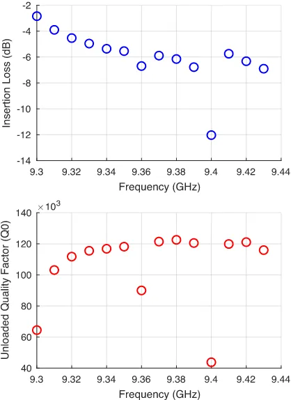
The results are shown in Fig. 16 where it can be seen that the maximum and minimum unloaded quality factors are 122 550 and 43 788, respectively, over the tuning range (130 MHz). The insertion loss (S21) varies between−2.84 and−12.03 dB over this range. Ignoring the frequencies (9.3, 9.36, and 9.4 GHz) where the wanted resonance interacts with an unwanted mode, the unloaded Q is above 100 000 and the insertion loss above
−7 dB. There may be other frequencies where this problem can occur because it is difficult to make high-Q measurements over such a broad frequency range.
A plot of insertion loss versus frequency with a narrow span of 1 MHz with the 3-dB points for the highest unloaded Q of 122 550 is shown in Fig. 17. The insertion loss (S21) was measured to be −6.15 dB at 9.38 GHz. The unloaded Q is
[image:9.612.51.560.313.530.2]Fig. 16. Plot of the measured insertion loss and unloaded quality factor (Q0)
[image:10.612.70.279.57.344.2]for the tuneable Bragg resonator. The cavity was tuned over a 130-MHz range.
Fig. 17. Plot of measured insertion loss versus frequency with a 1-MHz span showing an unloaded Q of 122 550.S21= −6.15 dB,S11= −9.13 dB,
andS22= −4.81 dB at 9.38 GHz.
field, high energy storage region, and radiation or losses in this section are likely to degrade the Q-factor. An absorbing boundary condition could be implemented in the 2.5-D field solver [25]. A narrow slot could then be modeled in the central air region and the effect of radiation losses investigated.
VII. DISCUSSION OFTEMPERATURESTABILITY The temperature dependence of a tuneable resonator can reduce the maximum allowable tuning range around a fixed center frequency because the center frequency will shift as a function of temperature.
The effect of this can be reduced by active temperature compensation and by varying the temperature coefficients of the materials used to construct the resonator. Based on the data sheet, the dielectric (alumina) used in this paper has a coefficient of thermal expansion (CTE) of approximately
+8.2 ×10⁻⁶/°C and the aluminum shield has a CTE of approximately+22.2×10⁻⁶/°C. The variation in the alumina dielectric constant with temperature is not known.
The cavity is also held together with 28 steel bolts, the torque on these is not fixed as these are adjusted to obtain maximum Q (minimum leakage) between the metal sections. This leakage is probably due to the imperfect flatness of the metal plates.
Calculating the temperature dependence of the resonant frequency is therefore nontrivial and further evaluation through measurement and modeling will be required.
VIII. CONCLUSION
In this paper, we have demonstrated a high-Q tuneable Bragg resonator with a tuning range of 130 MHz. The insertion loss S21 varies from−2.84 to−12.03 dB while the unloaded Q varies from 43 788 to 122 550 over the tuning range. At the center of the tuning range, there are unwanted modes approx-imately 9 MHz below 24 MHz above the center frequency.
The fitness function in the optimization algorithm could be modified to include mode to mode spacing as well as the magnitude of the input reflection coefficient. It may then be possible to find alternative plate arrangements that have a more desirable spurious mode response.
We believe that this combination of quality factor and tuning range is not possible with any other microwave resonators present in the literature. Broad tuning ultrahigh-Q cavities such as this one will enable versatile ultra-low phase noise tuneable oscillators offering broadband electromechanical course tuning and electronic fine tuning.
X-band oscillators with a fixed frequency Bragg resonator which have an unloaded Q of 200 000 are currently under investigation. Initial phase noise results for these oscillators are around−153 dBc/Hz at 10-kHz offset. The results are based on a measured residual flicker noise corner of around 26 kHz (an operating power noise figure of 8.1 dB including phase shifter/cable losses) and a PAVO at the input of the resonator of 11.5 dBm. These results are within 1 dB of the theory [27], [28]. Also, residual phase noise measurements of the active components are being measured using a broadband cross correlation phase noise measurement system [31].
ACKNOWLEDGMENT
The authors would like to thank J. Clapham for his help in the construction of the main cavity.
REFERENCES
[image:10.612.51.298.381.570.2][2] C. McNeilage, J. H. Searls, E. N. Ivanov, P. R. Stockwell, D. M. Green, and M. Mossamaparast, “A review of sapphire whispering gallery-mode oscillators including technical progress and future potential of the technology,” inProc. IEEE Int. Freq. Control Symp. Expo., Aug. 2004, pp. 210–218.
[3] B. S. Virdee, “Current techniques for tuning dielectric resonators,”
Microw. J., vol. 41, no. 10, pp. 130–138, Oct. 1998.
[4] A. Fox and L. A. Trinogga, “The electronic tuning and analysis of a slotted dielectric resonator filter,” inProc. ISAP, Chiba, Japan, 1996, pp. 949–952.
[5] A. N. Farr, G. N. Blackie, and D. Williams, “Novel techniques for electronic tuning of dielectric resonators,” inProc. 13th Eur. Microw. Conf., Nurnberg, Germany, Sep. 1983, pp. 791–796.
[6] P. R. Herczfeld, A. Daryoosh, C. D’Ascenzo, M. Contarino, and A. Rosen, “Optically tuned and FM modulated X-band dielectric resonator oscillator,” inProc. 14th Eur. Microw. Conf., Liège, Belgium, 1984, pp. 268–273. [Online]. Available: http://ieeexplore.ieee.org/ document/4132044/
[7] J. Gan and D. Xu, “Technique for optically tuning dielectric resonators,”
Electron. Lett., vol. 34, no. 22, pp. 2137–2138, Oct. 1998.
[8] P. R. Herczfield, A. S. Daryoush, V. M. Contarino, A. Rosen, Z. Turski, and A. P. S. Khana, “Optically controlled microwave devices and circuits,” inIEEE MTT-S Int. Microw. Symp. Dig., St. Louis, MO, USA, Jun. 1985, pp. 211–214.
[9] W. J. Keane, “YIG filters aid wide open receivers,”Microwaves, vol. 17, no. 8, pp. 295–308, Sep. 1980.
[10] C. A. Flory and R. C. Taber, “High performance distributed Bragg reflector microwave resonator,”IEEE Trans. Ultrason., Ferroelect., Freq. Control, vol. 44, no. 2, pp. 486–495, Mar. 1997.
[11] C. J. Maggiore, A. M. Clogston, G. Spalek, W. C. Sailor, and F. M. Mueller, “Low-loss microwave cavity using layered-dielectric materials,”Appl. Phys. Lett., vol. 64, no. 11, pp. 1451–1453, 1994. [12] C. A. Flory and H. L. Ko, “Microwave oscillators incorporating
high performance distributed Bragg reflector microwave resonators,”
IEEE Trans. Ultrason., Ferroelect., Freq. Control, vol. 45, no. 3, pp. 824–829, May 1998.
[13] J. Krupka, A. Cwikla, M. Mrozowski, R. N. Clarke, and M. E. Tobar, “High Q-factor microwave Fabry–Perot resonator with distributed Bragg reflectors,”IEEE Trans. Ultrason., Ferroelect., Freq. Control, vol. 52, no. 9, pp. 1443–1451, Sep. 2005.
[14] J. Krupka, M. E. Tobar, J. G. Hartnett, D. Cros, and J. M. L. Floch, “Extremely high-Q factor dielectric resonators for millimeter-wave applications,” IEEE Trans. Microw. Theory Techn., vol. 53, no. 2, pp. 702–712, Feb. 2005.
[15] J. Breeze, J. Krupka, and N. M. Alford, “Enhanced quality factors in aperiodic reflector resonators,” Appl. Phys. Lett., vol. 91, no. 15, p. 152902, 2007.
[16] J. Breeze, M. Oxborrow, and N. M. Alford, “Better than Bragg: Optimizing the quality factor of resonators with aperiodic dielectric reflectors,”Appl. Phys. Lett., vol. 99, no. 11, p. 113515, 2011. [17] S. Bale and J. Everard, “High-QX-band distributed Bragg resonator
uti-lizing an aperiodic alumina plate arrangement,”IEEE Trans. Ultrason., Ferroelect., Freq. Control, vol. 57, no. 1, pp. 66–73, Jan. 2010. [18] P. D. Deshpande, S. J. Bale, M. Hough, and J. Everard, “Highly tuneable
X-band Bragg resonator—Initial results,” in Proc. Joint Conf. IEEE Int. Freq. Control Symp. Eur. Freq. Time Forum, Denver, CO, USA, Apr. 2015, pp. 423–426.
[19] D. M. Pozar,Microwave Engineering, 3rd ed. Hoboken, NJ, USA: Wiley, 2005, pp. 284–287.
[20] D. M. Pozar,Microwave Engineering, 3rd ed. Hoboken, NJ, USA: Wiley, 2005, pp. 97–98.
[21] D. M. Pozar,Microwave Engineering, 3rd ed. Hoboken, NJ, USA: Wiley, 2005, pp. 18–19.
[22] S. J. Bale, “Ultra high Q resonators and very low phase noise measure-ment systems for low noise oscillators,” Ph.D. dissertation, Dept. Elect., York Univ., York, U.K., 2012.
[23] A. Taflove,Computational Electrodynamics: The Finite-Difference Time-Domain Method. Boston, MA, USA: Artech House, 1995.
[24] Y. Chen, R. Mittra, and P. Harms, “Finite-difference time-domain algorithm for solving Maxwell’s equations in rotationally symmetric geometries,” IEEE Trans. Microw. Theory Techn., vol. 44, no. 6, pp. 832–839, Jun. 1996.
[25] V. Rodriguez-Pereyra, A. Z. Elsherbeni, and C. E. Smith, “A body of revolution finite difference time domain method with perfectly matched layer absorbing boundary,”Prog. Electromagn. Res., vol. 24, pp. 257–277, 1999. [Online]. Available: http://www.jpier.org/PIER/pier. php?volume=24
[26] C. Wang, B.-Q. Gao, and C.-P. Deng, “Accurate study of Q-factor of resonator by a finite-difference time-domain method,” IEEE Trans. Microw. Theory Techn., vol. 43, no. 7, pp. 1524–1529, Jul. 1995. [27] J. Everard, Fundamentals of RF Circuit Design: With Low Noise
Oscillators. Hoboken, NJ, USA: Wiley, Dec. 2000.
[28] J. Everard, M. Xu, and S. Bale, “Simplified phase noise model for negative-resistance oscillators and a comparison with feedback oscillator models,” IEEE Trans. Ultrason., Ferroelect., Freq. Control, vol. 59, no. 3, pp. 382–390, Mar. 2012.
[29] J. K. A. Everard and C. D. Broomfield, “High Q printed helical resonators for oscillators and filters,”IEEE Trans. Ultrason., Ferroelect., Freq. Control, vol. 54, no. 9, pp. 1741–1750, Sep. 2007.
[30] Z. Ma and Y. Kobayashi, “Error analysis of the unloaded Q-factors of a transmission-type resonator measured by the insertion loss method and the return loss method,” inIEEE MTT-S Int. Microw. Symp. Dig., Seattle, WA, USA, Jun. 2002, pp. 1661–1664.
[31] S. J. Bale, D. Adamson, B. Wakley, and J. Everard, “Cross correlation residual phase noise measurements using two HP3048A systems and a PC based dual channel FFT spectrum analyser,” inProc. 24th Eur. Freq. Time Forum, Noordwijk, The Netherlands, Apr. 2010, pp. 1–8.
Simon J. Bale (M’05) received the M.Eng. and
Ph.D. degrees from the University of York, York, U.K., in 2004 and 2012, respectively.
He is currently a Research Fellow with the Depart-ment of Electronics, University of York. In the RF/microwave area, his research interests include high-Q microwave resonators, ultralow phase noise oscillators, and low-noise measurement techniques. In the evolutionary computing area, his research interests include microelectronic design optimization using bioinspired methods and techniques as well as nanoscale analog and digital designs.
Pratik D. Deshpande received the M.Sc. degree in communication engineering from the University of Manchester, Manchester, U.K., in 2011, and the Ph.D. degree in RF and microwave electronics from the University of York, York, in 2016.
He is currently an MMIC Design Engineer with Viper RF, focusing on high-power amplifiers, low-noise amplifiers, and phase shifters and attenuators up to Ka band using GaAs and GaN technologies.
Mark Hough received a Higher National Certifi-cate in electronics and communications engineering from York Technical College, Rock Hill, SC, USA, in 1990.
He is currently with the Department of Electronics, University of York, where he is involved in the area of Technical Support Services for teaching and research. The majority of his work is in the design and fabrication of electronic hardware and mechanical assemblies.
Stuart J. Porter (M’93) received the B.Sc. and D.Phil. degrees from the University of York, York, U.K., in 1985 and 1991, respectively.
Jeremy K. A. Everard(M’90) received the B.Sc. Eng. degree from the University of London (King’s College), London, U.K., in 1976, and the Ph.D. degree from the University of Cambridge, Cam-bridge, U.K., in 1983.
He worked in industry for six years at the GEC Marconi Research Laboratories, Great Bad-dow, Chelmsford, U.K., M/A-Com, Dunstable, U.K., and Philips Research Laboratories, Redhill, U.K., on radio and microwave circuit design. At Philips, he led the Radio Transmitter Project Group. He joined King’s College London as a “New Blood” Lecturer in 1983, where he taught RF and microwave circuit design, optoelectronics, and electromagnetism for nine years while leading the Physical Electronics Research Group. He became a University of London Reader in electronics at King’s College London in 1990 and a Professor of electronics at the University of York, York, U.K., in 1993. He has published papers on oscillators, amplifiers, resonators and filters, all optical switching, optical components, optical fiber sensors, and mm-wave optoelectronic devices and a bookFundamentals of RF Circuit Design with Low Noise Oscillators(Wiley). He has co-edited and co-authored a book on
gallium arsenide technology and its impact on circuits and systems, and he has contributed to a book on optical fiber sensors. He has filed patent applications in many of these areas. In the RF/microwave area, his research interests include the theory and design of low-noise oscillators using inductor capacitor, surface acoustic wave, crystal, dielectric, transmission line, helical and superconducting resonators, flicker noise measurement and reduction in amplifiers and oscillators, high-efficiency broadband amplifiers, high-Q printed filters with low radiation loss, broadband negative group delay circuits, and ultralow phase noise compact atomic clocks using laser probing and coher-ent population trapping. His research interests in opto-electronics include all optical self-routing switches that route data-modulated laser beams according to the destination address encoded within the data signal, ultrafast three-wave optoelectronic detectors, mixers, and phase-locked loops, distributed fiber optic sensors, and terahertz transmitters and receivers.