Phase-field modeling of crack branching and deflection in heterogeneous media

This is a repository copy of

Phase-field modeling of crack branching and deflection in

heterogeneous media

.

White Rose Research Online URL for this paper:

http://eprints.whiterose.ac.uk/152816/

Version: Submitted Version

Article:

Hansen-Dörr, A.C., Dammaß, F., de Borst, R. et al. (1 more author) (Submitted: 2019)

Phase-field modeling of crack branching and deflection in heterogeneous media. arXiv.

(Submitted)

© 2019 The Author(s). For reuse permissions, please contact the Author(s).

eprints@whiterose.ac.uk

Reuse

Items deposited in White Rose Research Online are protected by copyright, with all rights reserved unless indicated otherwise. They may be downloaded and/or printed for private study, or other acts as permitted by national copyright laws. The publisher or other rights holders may allow further reproduction and re-use of the full text version. This is indicated by the licence information on the White Rose Research Online record for the item.

Takedown

If you consider content in White Rose Research Online to be in breach of UK law, please notify us by

Phase-Field Modeling of Crack Branching and Deflection in Heterogeneous

Media

Arne Claus Hansen-D¨orra_{, Franz Dammaß}a_{, Ren´e de Borst}b_{, Markus K¨astner}a,c,∗

a_{Institute of Solid Mechanics, TU Dresden, Dresden, Germany}

b_{University of Sheffield, Department of Civil and Structural Engineering, Mappin Street, Sir Frederick Mappin Building, Sheffield S1 3JD, UK} c_{Dresden Center for Computational Materials Science (DCMS), TU Dresden, Dresden, Germany}

Abstract

This contribution presents a diffuse framework for modeling cracks in heterogeneous media. Interfaces are depicted by static phase-fields. This concept allows the use of non-conforming meshes. Another phase-field is used to describe the crack evolution in a regularized manner.

The interface modeling implements two combined approaches. Firstly, a method from the literature is extended where the interface is incorporated by a local reduction of the fracture toughness. Secondly, variations of the elastic properties across the interface are enabled by approximating the abrupt change between two adjacent subdomains using a hyperbolic tangent function, which alters the elastic material parameters accordingly.

The approach is validated qualitatively by means of crack patterns and quantitatively with respect to critical energy release rates with fundamental analytical results from Linear Elastic Fracture Mechanics, where a crack impinges an arbitrarily oriented interface and either branches, gets deflected or experiences no interfacial influence. The model is particularly relevant for phase-field analyses in complex-shaped, heterogeneous solids, where cohesive failure in the constituent materials as well as adhesive failure at interfaces and its quantification play a role.

Keywords: phase-field modeling, brittle fracture, diffuse modeling framework, heterogeneity, adhesive failure

1. Introduction

Crack propagation is one of the most severe mechanisms compromising the bearing capacity of engineering struc-tures. The phase-field approach to fracture has proven to be a powerful tool for the numerical prediction of crack propagation. The method allows for the description of complex failure mechanisms, such as crack nucleation and arrest, as well as branching and merging phenomena [1,2,3,4]. The concept is based on the variational approach to brittle fracture [5], which is consistent with the energetic criterion of Griffith [6]. The key idea of the phase-field method is the regularization of the underlying energy functional [7]: Cracks are approximated by an auxiliary field, often referred to as the crack phase-field. The phase-field variable continuously varies from the intact to the fully broken material state; cracks are regularized using a finite length scaleℓc. Furthermore, the approach allows for the

description of cracks with a non-conforming mesh, i.e. the element edges do not have to be aligned with the crack. Modern engineering materials often consist of several components, e.g. fibre-reinforced composites. As a separa-tion of these components can occur, the adhesive interfaces within a heterogeneous material can significantly influence the mechanical behavior of structures under external loading. Therefore, it is indispensable to account for interfaces in numerical simulations of fracture phenomena.

In the context of the Linear Elastic Fracture Mechanics (LEFM) analyses of He and Hutchinson [8,9], the interface is defined as a zone of infinitesimal width, which is assigned a fracture toughness that differs from the bulk material. Different setups were investigated, where a crack impinges a possibly inclined interface and either experiences no interfacial influence regarding the crack path or gets deflected. These fundamental and insightful investigations serve as analytical reference for numerical models, which incorporate interfaces in different manners.

∗_{markus.kaestner@tu-dresden.de}

Nomenclature

Latin symbols

a domain measure

A cross-sectional area

b domain measure

c domain measure

phase-field

C circular integration domain

d signed distance

D physical dimensions

E Young’s modulus

g degradation function ˜

gi configurational force G energy release rate

Gc fracture toughness

I functional

Ji crack driving force

ℓ regularization length scale

ni surface normal vector

r radius

s,t coordinates oriented to interface

t time

¯

ti given surface traction

ui,ui¯ displacement, given displacement

u displacement boundary condition

V volume

xi index notation of coordinates

¯

x=[ ¯xy¯]⊤ position of virtual crack tip

x,y cartesian coordinates

Greek symbols

α First Dundurs’ parameter

γ surface density

Γ surface

δ Diracdistribution

δ• test function for•

δi j Kroneckerdelta

∆ increment of . . .

εi j strain tensor η residual stiffness

ηf kinetic fracture parameter/viscosity

θ angle

κ external volume micro force

ν Poissonratio

ξi micro force traction π internal volume micro force

σi j stress tensor

Σi j energy momentum stress tensor ϕ inclination angle

ψ free energy density

Ψ free energy

Ω domain

Sub-/superscripts

+ tensile part

− compressive part

ˆ

1,2 material numbering act actual . . .

b bulk . . . bottom

c crack/phase-field . . . C constant boundary condition def deformation . . .

dis dissipation . . . el elastic . . .

E exponential regularization

G Gaussian-like regularization

H Heaviside-like description

sharp Heavisidejump i interface . . .

ℓc regularized crack/phase-field . . . ℓi regularized interface . . .

len length along interface max maximum . . . min minimum . . .

modE varying Young’s modulus . . .

n increment number

N near-field boundary condition ref reference value

s side

t natural boundary condition

t top

th threshold tip crack tip . . .

⊤ transposed

T hyperbolic tangent boundary condition hyperbolic tangent regularization

u essential boundary condition

Abbreviations

BC boundary condition

FEniCS open-source finite element package LEFM Linear Elastic Fracture Mechanics PETSc numerics library

An approach quite close to the LEFM view on the interface was proposed by Paggi and Reinoso [10] and later Guill´en-Hern´andez et al. [11]. They introduced a phase-field model for brittle fracture, where the interface is captured by cohesive zone elements: The cohesive zone approach is extended so that the phase-field affects both, the bulk material and interface stiffness. Good agreement of their hybrid model and the analytic investigations of He and Hutchinson [8] was achieved. A drawback of the model is the necessity of a mesh-conforming interface, i.e. cohesive zone elements have to be introduced along the interface. An extension to moving interface problems as apparent in phase transitions is thus not straightforward.

Nguyen et al. [12,13] proposed a phase-field model for interface failure, where the relations for a standard cohesive zone model are applied to a regularized interface. The regularization is inspired by the crack surface density and takes the same form. Instead of the fracture toughness, a cohesive energy depending on the regularized displacement jump captures the energetic contribution to the total energy. In contrast to a classical cohesive zone model, the interface can be described in a non-conforming manner using a level-set, which can be generated from CT images.

Schneider et al. [14] presented a multiphase-field model capable of depicting cracks along the interface separating solid phases. By using a multiphase-field model, the interface is accounted for by a grain boundary energy, which is, however, different from the fracture toughness. For a varying grain boundary energy, the authors reproduced phenomena similar to those considered by He and Hutchinson [8]. A quantitative comparison is not straightforward because the fracture toughness, present in [8], was not used in [14] to characterize the fracture properties of the interface. The advantage of the multiphase-field model is the capability to describe non-conforming interfaces in a framework, which already allows for phase transitions and thus, a possible evolution of the interface itself.

Hansen-D¨orr et al. [15,16,17] have presented the concept of a regularized, diffuse interface: In the context of the fracture phase-field, the regularized interfaceΓℓi_{is defined as anarrowsubdomain of a solid with a small – but finite –}

characteristic widthℓi, which is assigned an interface fracture toughnessGic. As the length scales of the interface and

crack interact, the effective fracture toughness of the interface depends on the characteristic length scalesℓi andℓc,

and on the fracture toughness of the surrounding bulk material. In [17], a compensation of this effect by means of definition of a modified numerical interface fracture toughness was proposed. The advantage of this approach is simplicity, while keeping accuracy. Once the compensation has been determined, a non-conforming interface can be embedded. This approach can be extended to moving interfaces, where evolution equations for the interface have to be implemented [18,19].

The characteristic interface widthℓi is closely related to experimental work of Park and Chen [20], and Parab

and Chen [21]. In both papers, projectiles are fired at brittle solids to provoke dynamic crack propagation towards a perpendicular interface. The interface has a varying, finite width and is made of an adhesive, gluing two brittle solids together. Depending on the interface width, different fracture phenomena occur. The same behavior is observed in the present paper and underlines the fact, that the characteristic width of the interface is not a purely numerical parameter. This contribution extends the modeling approach developed by Hansen-D¨orr et al. [17] to obtain a more numer-ically robust description of the interface and to incorporate elastic heterogeneities. The first issue is addressed by introducing two continuous regularization functions that characterize the interface. These functions which smoothly describe the transition from the bulk to the interface fracture toughness, are considered instead of an actual material stripe assigned the interface fracture toughness. Elastic heterogeneities are captured by postulating an approxima-tion for the elastic constants in the interface region depending on the surrounding bulk materials properties. The consequences of different interface regularizations are discussed in detail. The model is validated by qualitative and quantitative comparisons to analytical results from LEFM [8]. In order to obtain a controlled crack growth through or along the interface,surfing boundary conditions[22] are applied. For a quantitative insight into the failure mecha-nisms, the concept of configurational forces is exploited [23,24].

0

δ(x)

δ

x

(a) Discrete crack surface representation

0 1

0 2ℓc

c

x

(b) Regularized crack surface representation

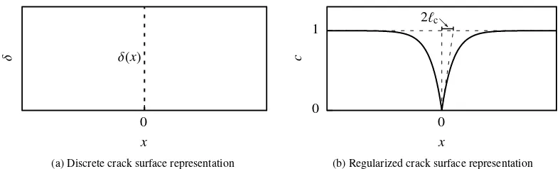
Figure 1: In(a), the location of the sharp crack is described by the Diracdistribution. The regularized representation using an exponential function

is depicted in(b). The length scale parameterℓccontrols the width of the transition region fromc=0 toc=1.

2. Phase-field modeling of regularized material heterogeneities

2.1. Introduction of crack surface density

The idea of phase-field modeling of fracture is the introduction of an additional scalar fieldc ∈ [0,1], which implements a smooth transition from intact (c = 1) to fully broken (c = 0) material. The additional field cis referred to as the phase-field in view of the resemblance of the concept to classical phase-field models. Suppose a one-dimensional rod withx ∈ [−∞,∞] of cross-sectional areaAwhich is cracked at the centre at x = 1 mm: The crack location can be fixed using a Diracdistribution, cf. Figure1a, and the total crack surfaceΓccan be obtained by integration over the domain

Γc= Z

Ω

δ(x) dV =

∞

Z

−∞

δ(x)Adx=A, (1)

yielding the intuitive resultΓc=A. The motivation to describe the crack surface in a regularized manner arises in the context of finite element analyses. The smooth functioncenables the use of non-conforming meshes, which obviates the need for remeshing in case of crack propagation. Following Bourdin et al. [1] the Diracdistribution is regularized using an exponential shaped function

c(x)=1−exp |x|

2ℓc

!

(2)

yielding a representation, which is depicted in Figure1b. The characteristic length scaleℓc controls the maximum gradient of the regularization, which has to be resolved in a finite element implementation.

It has been shown [2] that a functional

Ic,c′= Z

Ω

1 4ℓc

h

(1−c)2+4ℓc2 c′2

i

dV (3)

can be found, where Equation (2) is the solution to the Euler-Lagrange equation forI[c,c′_{]→ min andc}′_=dc/dx, subject to the boundary conditionc′_{(x → ±∞) =0. Note, that inserting Equation (2) into (3), in analogy to} Equa-tion (1), yieldsI = A = Γℓc_{, which is whyΓ}ℓc _{is used below instead of I. A three-dimensional generalization is}

obtained by replacingc′by the gradient

Γℓcc,c,i=

Z

Ω

1 4ℓc

h

(1−c)2+4ℓc2c,ic,i

i

| {z }

γℓc

dV, (4)

whereγℓc _{is referred to as crack surface density, cf. [2]. Herein, the summation convention and (•)}

2.2. Governing differential equations andClausius-Duheminequality

The local form of the momentum balance, neglecting volume forces and inertia, reads

σi j,i=0 where σi j=σji, (5)

with the Cauchystress tensorσ_{i j}, subject to the boundary conditions

σi jni=t¯j on ∂Ωt and

ui=u¯i on ∂Ωu,

(6)

where the boundary∂Ω =∂Ωt∪∂Ωuhas been decomposed into a part∂Ωt with natural boundary conditions and a

part∂Ωuwith essential boundary conditions, and∅=∂Ωt∩∂Ωu. The symmetry of the stress tensor follows from the

angular momentum balance. The stress is energetically conjugate to the strain rate ˙εi j, with the strain defined as

εi j=

1 2

ui,j+uj,i

, (7)

in a geometrically linear setting, and the displacementui.

Following Borden [25, p. 63ff.] or Kuhn [26, p. 41ff.], micro forces are introduced as energetically conjugate to the phase-field rate ˙c. The according conservation equation in the local form reads

ξi,i+π+κ=0 , (8)

whereξi is the micro force traction andπandκ are internal and external volume forces, respectively. After some

manipulations and consideration of the first and second laws of thermodynamics, the Clausius-Duheminequality

"

σi j(εkl,c)− ∂ψ ∂εi j

#

˙

εi j+

"

ξi

c,c,j,c˙

− ∂ψ

∂c,i

#

˙

c,i−

"

πc,c,j,c˙

+∂ψ

∂c

#

˙

c≥0 (9)

is derived. Here, the argument of Gurtin [27] has been employed, that the free energy densityψεi j,c,c,k

must not be a function of ˙c. The dependencies ofψare dropped above and below for sake of readability. Furthermore, ˙εi j and

˙

c,iappear linearly: If Equation (9) shall hold for any admissible ˙εi jand ˙c,i, the constitutive relations

σi j(εkl,c)= ∂ψ ∂εi j

and (10)

ξi

c,c,j,c˙

= ∂ψ

∂c,i

(11)

can be deduced. Following the argument of Gurtin [27] or Kuhn [26, p. 41ff.], the last term can be satisfied if

πc,c,j,c˙

=−ηfc˙− ∂ψ

∂c , (12)

whereηf ≥0 serves as a kinetic fracture parameter or viscosity. Inserting Equations (11) and (12) into Equation (8),

a Ginzburg-Landau-type equation

ηfc˙= ∂ψ ∂c,i

!

,i

−∂ψ

∂c (13)

is obtained. As the phase-fieldcis not influenced by any external quantity directly, a zero external micro volume forceκ=0 and the homogeneous boundary condition

ξi

c,c,j,c˙

ni=0 on ∂Ω (14)

2.3. Constitutive modeling of material response

The constitutive modeling approach follows an additive split of the total free Helmholtzenergy

Ψ=

Z

Ω

ψdV = Z

Ω

ψeldV+ Z

Ω

ψℓcdV (15)

into an elasticψeland a phase-fieldψℓc _{contribution. For the elastic term, the widely used tensile split [2]}

ψel=g(c)ψel_0,++ψel_0,− with ψel₀ = E(xl)ν

2(1−2ν)(1+ν)(εkk)

2₊ E(xl)

2(1+ν)εi jεi j (16)

has been adopted. Only the tensile partψel_0,+is degraded using the degradation functiong(c)=c2+ηto prevent crack forming under pressure. A small residual stiffnessη =10−6 _{is maintained for the fully degraded (c=0) state. The}

Young’s modulusE(xl) may exhibit a spatial dependence, cf. Section2.5.2, while the Poissonratioνis assumed to be constant in the remainder of this paper. The tensile split does not fully degrade the material under shear [28]. A remedy to this issue is the physically based split [29]. Possible impacts on the results are discussed below.

The energy apparently stored within the phase-field contribution takes the form

ψℓc =Gc(xl)

4ℓc

h

(1−c)2_+4ℓ c2c,ic,i

i

=Gc(xl)γℓc, (17)

which stems from the energetic criterion of Griffith [6]. It is noted, that the fracture toughnessGc(xl) may exhibit a

spatial dependence, see Section2.5.1.

With the constitutive model at hand, it is possible to deduce more specific expressions for the stress

σi j =g(c) ∂ψel_0,+

∂εi j

+∂ψ

el 0,−

∂εi j

, (18)

the evolution equation for the phase-field

ηfc˙= Gc(xl)

2ℓc

+2ℓc Gc(xl)c,i,i−c Gc(xl)

2ℓc

+2ψel_0,+

!

(19)

and the corresponding boundary condition

c,ini=0 on ∂Ω (20)

from Equations (10), (13) and (14).

In order to prevent existing cracks from healing, an irreversibility constraint has to be imposed. There are two widespread approaches, thedamage-like andfracture-like irreversibility condition. The former one interprets the phase-field as damage variable and requests ˙c ≤0 in every material point. This can be achieved by introducing a history variable [3]. The latter approach allows for local reversibility and does not constraint the phase-field before it reaches a critical threshold close to zero [4]. Then, a Dirichletboundary conditionc=0 is set at the corresponding location. The advantage of thefracture-likeconstraint is, that the dissipated energy associated with the crack surface is not overestimated [30]. In this contribution, the latter approach is chosen with a threshold ofcth =0.03. A study

for different values ofcthdid not reveal any significant differences. As well, studies with finer discretizations revealed

no further influence.

2.4. Weak form and finite element implementation

The weak forms of the partial differential equations (5) and (19) are derived by multiplication with test functions

δujandδc, and integration over the whole domain,

0= Z

Ω

σi j,iδujdV and (21)

0= Z

Ω

"

Gc(xl)

2ℓc

+2ℓc Gc(xl)c,i,i−c Gc(xl)

2ℓc

+2ψel_0,+

!

−ηfc˙

#

Integration by parts and making use of the divergence theorem yields

0= Z

Ω

σi jδuj,idV−

Z

∂Ωt

¯

tjδujdA and (23)

0= Z

Ω

"

Gc(xl)

2ℓc

−c Gc(xl)

2ℓc

+2ψel_0,+

!

−ηfc˙

#

δc−2ℓcGc(xl)c,iδc,idV+

Z

∂Ω

2ℓcGc(xl)c,iniδc

| {z }

=0,cf. Eq. (20)

dA. (24)

A time discrete form is obtained, by replacing the phase-field rate in Equation (24) using an Eulerbackward scheme

˙

c≈c−

n_c

∆t , (25)

wheren_{cis the converged phase-field value of the previous increment and∆tis the time step.}

The open-source finite element package FEniCS and the numerics library PETSc [31] allow for an efficient par-allelized solution of differential equations. An important ingredient of the framework is the so-calledUnified Form

Language(UFL) [32], a python-based language for mathematical expressions. The implementation is carried out by

stating the weak form and all necessary constitutive relations using UFL. Special attention has to be paid to the neces-sary spectral decomposition of the strain tensor due to the tensile split. From that, a parallelized code for the solution of the finite element system is automatically generated [33,34]. The resulting non-linear, time-discrete equations are solved using a fully coupled, monolithic approach. A heuristic adaptive time-stepping scheme is employed, which reduces the time step, if the Newton-Raphsonscheme reaches no convergence within 70 iterations and increases the time step if convergence is reached within four iterations. Spatial convergence has been verified. Along the interface and the crack path, the mesh is refined such that the characteristic element length is five to eight times smaller thanℓc.

2.5. Interface modeling in the context of regularized heterogeneities

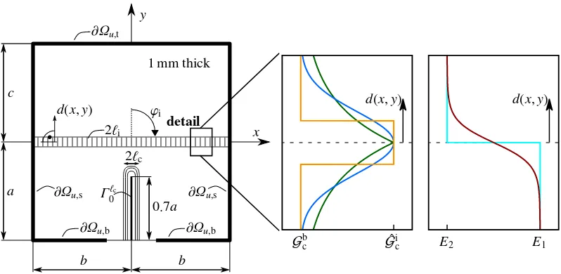
In the context of LEFM, interfaces are mostly introduced as infinitesimal layers of D−1 physical dimension, whereDis the dimension of the considered domain separated by the interface. Such a description is also chosen in the work of He and Hutchinson [8,9], who investigated crack deflection and branching at interfaces. Surrounded by two, possibly dissimilar, bulk materialsi=1,2 with elasticEi, νiand fractureGbcmaterial parameters, the interfaceΓi

is only assigned an interface fracture toughnessGi_c, cf. Figure2a. A crackΓcemerging along the interface hasD−1 physical dimension, too.

Hansen-D¨orr et al. [15,16,17] have introduced a regularized interface model which allows for non-conforming interfaces within a regular mesh. In analogy to classical phase-field models, the interface is regularized and defined as a subdomainΓℓi_{ofDphysical dimensions, which separates at least two other subdomains of materials with possibly}

dissimilar elastic properties. The interface mid-surface is identical to the discrete interfaceΓi. The difference of the interface Γℓi _{to other sub-structures is, that one physical dimension is considerably smaller than the smallest}

characteristic lengths of every other subdomain (except from other interfaces). This property is callednarrowand is quantified by introducing the length scaleℓi, which measures the width in the direction of the signed distanced, cf.

Figure2b. It is further assumed, that the elastic energy stored within such a regularized interface is negligibly small compared to non-interfacial subdomains. Thus, in analogy to the LEFM description, the interface is not explicitly assigned exclusive elastic parameters but also values depending on the surrounding bulk materials. Despite this simplification the fracture toughness Gi_c is still relevant and can significantly influence the macroscopic cracking behavior of a structure, even if the interface width is macroscopically not recognizable. A crack along the interface is regularized, too, and becomes a phase-field crackΓℓc_{with the characteristic lengthℓ}

c.

2.5.1. Incorporation of the interface by means of a fracture toughness reduction

An interface, which is schematically depicted in Figure2b, can be described using a Heaviside-like function for the fracture toughness

GH_c(d,Gb_c,Gi_c)=       

Gb

c for|d|> ℓi Gi_c for|d| ≤ℓi

Gb

c Gbc

Gb

c Gbc

Γc Γi,Gi_c

Γi,Gi_c

(a) Intact and broken interface according to LEFM [8]

d 2ℓi 2ℓc d

2ℓi

Gb_c Gb_c

Gb_c Gb

c Γℓc Γℓi_,Gi

c Γℓi_,Gi

c

(b) Intact and broken interface in a regularized setting

Figure 2: Intact and partially cracked interface for a 2D specimen: The interfaceΓiin LEFM is depicted by a line with a fracture toughnessGi_c different from the bulk material fracture toughnessGb

c,(a)left picture. Failure leads to a sharp crackΓc,(a)right picture. For a regularized interface Γℓi _{according to [17], the zone, where the fracture toughness deviates from}Gb

c, has a finite width. The regularization is schematically depicted

by the grey hatched area,(b)left picture. The parameterℓimeasures the width along the direction of the signed distanced. Failure leads to a regularized, phase-field crackΓℓc_{with characteristic lengthℓc,(b)right picture.}

within the whole domain. The spatial dependence ofGH_c is implicitly incorporated by the signed distanced, which measures the shortest distance from every point to the interface midline. This description was used by Hansen-D¨orr et al. [17], where it was shown that non-conforming interfaces can be described, despite the jump of the fracture tough-ness, which may occur within an element. However, the sharp switch between two fracture toughness values nega-tively influenced the convergence of the numerical solver. Besides the Heaviside-like description, an exponentially-shaped

GE_c(d,Gb_c,Gi_c)=Gb_c−Gb_c− Gi_c exp

"

−|d|

2ℓi

#

(27)

and a Gaussian-like

GG_c(d,Gb_c,Gi_c)=Gb_c−Gb_c− Gi_cexp

     

−

d

2ℓi

!2

    

 (28)

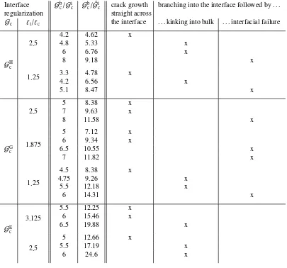
function are investigated. All three regularization functions1_{are depicted in Figure3a. The comparison clearly reveals,}

that the regularizationsGG_c andGE_c introduce a transition zone, which is larger thanℓi. However, in the context of the

regularized phase-field model, the lengthℓican still be identified as characteristic interface width in analogy to the characteristic crack lengthℓc. Additionally, the differentiation of the bulk material and the interface is softened by

introducing a continuous regularization: The interface is no longer an additional material stripe, which can clearly be identified, but a diffuse region.2

2.5.2. Incorporation of elastic heterogeneities near the interface

In the proposed model, the interface formally has the same number of material parameters as the surrounding bulk material. In earlier investigations with the model [16,35], only elastically homogeneous cases were investigated. The elastic constants of the two bulk materials were also applied within the interface even if it was in principle possible to consider completely different elastic constants, in a similar fashion as in Equation (26). However, as outlined above, the deformation energy of the interface is assumed to be negligibly small compared to the bulk materials’ deformation energy. This description is consistent with the assumption of analytic LEFM calculations [8], where the

D−1-dimensional interface neither has elastic properties.

In this work, the interface is interpreted as a transition zone with respect to the elastic material parameters. In principle, the transition could be modeled using a whole variety of different functions. In this work, only the Young’s modulus is allowed to vary, while the Poissonratioνis assumed constant for the present investigations. The modulus follows a hyperbolic tangent-like shape

ET(d)= E2−E1

2 tanh

"

d ℓi

#

+1

!

+E1. (29)

1_{In the context of the fracture phase-field, the authors understand the regularization of the interface as increase of its dimension, i.e. fromD−1}

in LEFM toDas in the present model within aD-dimensional domain.

2_{Referring to Figure2bthis means, that the grey stripe has to be understood as a symbol for the interface regularization and not a sharp}

Gi_c Gb_c

−4 −3 −2 −1 0 1 2 3 4

d/ℓi

-GH_c

-GG_c

-GE_c

(a) Regularization of the fracture toughness

E1 E2

−4 −3 −2 −1 0 1 2 3 4

d/ℓi

-EH

-ET

(b) Regularization of the Young’s modulus

Figure 3: Regularization curves for the material parameters:(a)depicts the fracture toughness distribution for the different functionsGH_c,GG_c and GE_c. The signed distanced(x,y) measures the shortest distance from any point within the domain to the interface midline.(b)depicts the spatial distribution of the Young’s modulusEHandET. In both plots, the location of the interface midlined/ℓ_i=0 is highlighted by a dashed

-line.

For some investigations, the smooth Young’s modulus transition is compared to the sharp limit, which reads

EH(d)=       

E2 ford>0

E1 ford≤0 .

(30)

It is further noted, that the length scales for the fracture toughness and Young’s modulus regularizations are both chosen in dependence ofℓi. Generally, these values could be independent from each other. However, it makes sense

to choose them in the same order of magnitude because they govern the spatial discretization, too. The functionsEH

andETare depicted in Figure3bforE2>E1, but not restricted to this condition.

The concept of regularizing jumps in the elastic constants according to Equation (29) is not new and has widely been used in literature, for example Schneider et al. [36], Mosler et al. [18] and Kiefer et al. [19], where a phase-field model is used to describe phase transitions. Equation (29) can thus be understood as a static phase-field. The assumption of such a transition might however lead to unwanted behavior in the vicinity of the interface as just stated. Physically not reasonable effects like an exaggerated, interfacial energy [36] or a violation of the mechanical jump conditions [36,18] may result. A possible solution is the so-called partial rank-I relaxationand accounts for the mechanical equilibrium in every material point.

In this contribution, no such approach is implemented at the cost of possible inaccuracies near the interface. The reason is that the combination of the tensile split introduced in Section2.4and apartial rank-I relaxationis non-trivial. The error which is made, is quantified below by a comparison to results obtained with a sharp, mesh-conforming elastic jumpEH_.

2.6. Configurational forces and link to energy release rate

The scope of this work is not only the qualitative analysis of various crack patterns in heterogeneous materials but also the quantification of the so-called crack driving forces, which lead to the aforementioned and yield a deeper understanding of why and when branching and deflection occur. Rice [37] and Cherepanov [38] developed the concept of a path independent integral, theJ-integral. The evaluation serves as an alternative way to calculate the energy release rateGin LEFM. Later, theJ-integral was generalized for multidimensional analyses, cf. [39,40,41]. For the specific application within a coupled mechanical crack phase-field framework, Kuhn and M¨uller [4,26,23] introduced a generalized configurational force balance, which is closely related to the generalizedJ-integral, to account for heterogeneities within the material in the determination of the energy release rate. The configurational force balance of the deformation energy

enables the computation of the crack driving forces. The individual contributions break down as follows. The defor-mation energy contribution

Σ_{i j}def=ψelδi j−uk,iσk j (32)

is identical to the integrand of the generalized J-integral, cf. [41]. The contribution of varying elastic material parameters manifests itself in

˜

gmodE_i =−∂ψ

el

∂xi

_explicit

, (33)

accounting for the explicit spatial dependence – in this work due to a varying Young’s modulus. The influence of the dissipative, viscous term is incorporated in

˜

gdis_i =ηfc c˙ ,i. (34)

Following Kuhn [23], the crack driving force

J_itip=−

Z

C ˜

gtip_i dV (35)

can be calculated by integrating over a circular volume of unit thickness

C=nx,y

(x−xtip)2+(y−ytip)2≤r2

o

(36)

with radiusrcentred at the crack tip [xtip ytip]⊤. The numerical evaluation is based on the weak form of Equation (31)

to avoid the calculation of the divergence, cf. [23]. In analogy to LEFM,J_itipcan be named generalizedJ-integral. In contrast to the classicalJ-integral it can be applied to locally heterogeneous structures. For the sake of simplicity, only the most important implications and relations have been mentioned here.

In general, the choice ofCmay influence the results of Equation (35), especially, when the radius is chosen too small or larger than the simulation domain. In order to arrive at an appropriate decision, the integral is evaluated for many different radii and the results are compared concerning converged integral component values. These components

J_itip,i=x,y, now reflect the energy release rates with respect to the chosen coordinate frame, which is why the term

energy release rateis used in the remainder of this paper for the discussion of individual components ofJ_itip. In this

work, a comparison of different radii revealedr=0.35 mm to be a good choice.

2.7. Interaction of regularization length scales

Hansen-D¨orr et al. [15,16,17] have observed that for homogeneous elastic properties and a fracture toughness variation according toGH

c, a straight mode-I crack does not propagate for a critical energy release rate equal to the

fracture toughness of the interfaceGi

c, but a higher valueG i,act

c betweenGicandGbc. The exact value of the actual

fracture toughness of the interface depends on the ratiosGb

c/Gic,ℓi/ℓcand the exact functionGHc,GGc orGEc which is

used.

The reason for this discrepancy is the interaction of the crack and the interface regularization. If the characteristic length of the interfaceℓiis in the same order asℓc, the phase-field for a cracked interface also protrudes into the bulk

material, which has a higher fracture toughness. This regularization induced exaggeration of the interface fracture toughness can be corrected in order to obtain the correct value Gi_c for a crack propagating along the interface by applying a lower, compensated numerical interface fracture toughness ˆGi_cin combination withGb_cfor the bulk material. For this purpose, a parameter study for variousGb_c/Gi_candℓi/ℓcsimilar to [17] has been carried out and the resulting

ratiosGb_c/Gi,actc for which Gbc/Gi,actc < Gbc/Gicholds, are recorded. They resemble discrete points of the functional

relation

Gb_c

Gi,act_c = f Gb_c

Gic ,ℓi

ℓc

!

. (37)

In the simulations,

Gb_c

Gi,actc !

=G

b c Gi c

= f G

b c

ˆ

Gi c

,ℓi ℓc

!

1 4 7 10 13 16 19

1 3 5 10 15 20

G

b c/

G

i c

Gb_c/Gˆi_c

(a) Heaviside-like description

1 3 5 7 9 11 13

1 3 5 10 15 20

G

b c/

G

i c

Gb_c/Gˆi_c

(b) Gaussian-like regularization

1 2 3 4 5 6 7

1 3 5 10 15 20

G

b c/

G

i c

Gb_c/Gˆi_c

(c) Exponential regularization

-ℓi/ℓc=3.125

-ℓi/ℓc=2.5

-ℓi/ℓc=1.875

-ℓi/ℓc=1.25

-ℓi/ℓc=0.625

Figure 4: Compensation of the length scale interaction ofℓi andℓc: A phase-field crack within the interface, whereℓi/ℓcis reasonably small,

experiences an influence of the surrounding bulk material fracture toughness, which is why the actual fracture toughness of the interface takes values betweenGi_candGb_c. Depending on the regularization(a)–(c)and the ratiosGb_c/Gi_candℓi/ℓc, a compensated fracture toughness ˆGi_ccan be determined, which accounts for the bulk material influence and leads to an interfacial crack resistance ofGi_c. The corresponding compensation plots are given in this figure. The exact procedure is described in the text and indicated in(b)with arrows and a brown, dashed interpolation line.

is required, i.e. the crack propagates along the interface forGc =Gic. Note that the compensated interface fracture

toughness ˆGi_c now appears in f. Thus, for a fixedℓi/ℓc, the right part of Equation (38) can be used to obtain the

compensated interface fracture toughness ˆGi_cby inversion of the function f. Since f, depicted in Figure4for every interface regularization, is not available in a continuous form, an alternative, graphical way has been chosen.

The graphical compensation is illustrated in the following for the Gaussian-like regularizationGG

c. Assume, it is

used to achieve the ratiosGb_c/Gi_c=6 andℓi/ℓc =1.25. The user now draws a horizontal, brown arrow in Figure4b

meeting the ordinate atGb_c/Gi_c=6. As the horizontal arrow does not meet a symbol ofℓi/ℓc=1.25 exactly, a brown, dashed interpolation line is drawn between the two adjacent symbols. The intersection of the horizontal arrow and the symbol/interpolation line of the ratioℓi/ℓc=1.25 marks the point, where a vertical arrow starts and runs down to the

abscissa, where the ratioGb

c/Gˆic ≈14.31 can be found and has to be applied within the simulations. In other words,

the fracture toughness regularization is slightly modified and now readsGG

c(d,Gbc,Gˆic) instead ofGGc(d,Gbc,Gic). Of

course, more sophisticated interpolation schemes are possible based on the data lying behind the plot.

The presented compensation approach, which is applied in the ensuing simulations on crack branching and de-flection, also works for the two other regularizations, where according compensation plots, Figures4aand4c, are provided. By comparing the three figures, a crucial difference becomes clear. For the same length scale ratios, dif-ferent values for the compensated interface fracture toughness have to be applied. In other words, if the interface regularization does not implement low fracture toughness values over a wide range across the interface, a compara-bly lower compensated interface fracture toughness has to balance the bulk fracture toughness influence. This effect increases from the Heaviside-like to the Gaussian-like to the exponential description and for the latter one, the satu-ration effect, which can be observed for every regularization, becomes the strongest, which is clearly a limitation. Its implications are discussed in Section3.

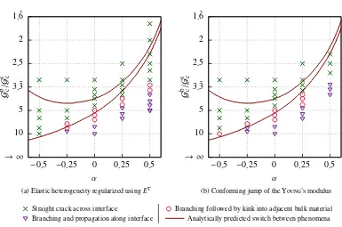
3. Crack branching and deflection at interfaces

The model presented above has been applied successfully to crack propagation along interfaces and it has been shown that the compensation is necessary for a quantitative comparison of crack driving quantities [17]. In this contribution, the setup is extended to a crack approaching an interface under a certain angleϕi. Depending on the bulk

y

x

b b

a c

0.7a

2ℓc

2ℓi ϕi

∂Ωu,b ∂Ωu,b

∂Ωu,s ∂Ωu,s

∂Ωu,t

Γℓc 0 d(x,y)

detail 1 mm thick

ˆ

Gi_c Gb_c

d(x,y)

E1 E2

d(x,y)

Figure 5: The general setup for the four different studies is sketched on the left. The regularized interface is schematically depicted by the grey hatched region, which may be inclined by a certain angleϕi. The interface regularization lengthℓiis no longer the exact width of the gray region

as it was in Figure2b, because not only the Heaviside-like descriptionGH_c is used. The signed distance_dfrom the interface is perpendicular to

the interface. The material parameters are assigned according to the regularization functions depicted on the right, using values ofE1,E2, ˆGi_cand Gb_c. Note, that the compensated interface fracture toughness ˆGi_cis used in all simulations to compensate the bulk material influence as described in Section2.7. Thedetailaround the vertically hatched interface area is magnified on the right, where the regularization plots from Figure3are shown. The initial crack is depicted byΓℓc

0. The bold marked boundary is decomposed into the bottom∂Ωu,b, the sides∂Ωu,sand the top∂Ωu,t.

These definitions are used below for applying the boundary conditions. It is noted, that homogeneous Neumannboundary conditions are applied in

the vicinity of the crack, i.e. forx∈[−0.2a,0.2a] andy=−a.

setups which are dealt with below: Depending on the choice of the Young’s moduliE₁andE₂, the bulk material and interface fracture toughnesses,Gb_candGi_crespectively, and the interface inclination angleϕi, four setups –

perpendicu-lar or inclined interface and homogeneous or heterogeneous elasticity – serve as benchmarks. The Poissonratio is not varied within the domain and the simulations have been conducted in a plane strain setting. For the investigations with a perpendicular interface, the domain measures area =b =c=1 mm. For the inclined interface, different domain measuresa =b/2=c/3=1 mm are chosen to avoid that the interface passes through the edges of the specimen for the anglesϕiunder consideration.

He and Hutchinson [8] have conducted their analytical investigations by assuming a symmetric far-field load in thex-direction. From that, the appropriate choice of the boundary conditions for the finite element model is not trivial. Hence, different types have been investigated for the first of the four studies, see Section3.1.1, and the choice for the other three studies is made based upon this.

In addition to the investigation of the boundary condition, all interface regularization functionsGH

c,GGc andGEc are

compared for the first study with a homogeneous Young’s modulus. Any influence arising from the regularization for the elastic heterogeneityET_{is avoided in this way.}

All simulations presented within this paper are conducted assumingℓc=15µm. The fracture toughness of the bulk

material is set to the constant valueGb_c =2.7 N mm−1 _whileGi

cis adapted according to the fracture toughness ratio Gb_c/Gi_cwhich is varied in order to study different fracture phenomena. Similarly, E1 = 210 kN mm−2 is considered

and for the investigation of elastic heterogeneity, different values ofE2are defined. A constant Poissonratioν=0.3 is assumed. The maximum and minimum time steps are∆tmax =8·10−2s and∆tmin=1·10−9s, respectively, and a

viscosityηf =10−5kN mm−2s−1is applied. In order to investigate the impact of this numerically motivated parameter,

a convergence study has been carried out. For this purpose,ηf =10−6kN mm−2s−1andηf =10−4kN mm−2s−1were

considered. The effect of the viscosityηf=10−5kN mm−2s−1on the simulations appeared to be rather small, and has

3.1. Homogeneous elasticity and crack perpendicular to interface

3.1.1. Comparison and quantification of boundary condition influences

In analytical investigations, failure phenomena are often analyzed neglecting boundary effects. For instance, He and Hutchinson [8,9] have considered a crack within an infinitely large domain and assumed a far-field loading. In contrast, a boundary condition has to be applied to a domain of finite size, when failure is investigated numerically. The boundary condition should be chosen such that it does not exclude certain failure modes. Unlike a far-field load, the boundary condition applied in a numerical model can influence the simulated crack path. In order to obtain numerical results comparable to the analytical investigations of He and Hutchinson [8,9], a boundary condition which causes a crack propagation similar to that caused by a far-field load should be chosen. Therefore, numerical results for different displacement boundary conditions and fracture toughness ratiosGb_c/Gi_ccan be compared in the following study.

Owing to its simplicity, a constant displacementuCinx-direction on the side edges∂Ω_u,s,

uC=uC

reft sign(x)

"

1 0

#

, (39)

is considered first. While the vertical component of the displacement is prevented on the boundary∂Ωu,s, the horizontal

component is increased proportionally with timetanduC_ref=4µm/s.

As it results in more steady, i.e. better controllable crack growth, the concept of the so-calledsurfing boundary

condition[22] is exploited. The key idea of this approach is to introduce a virtual crack tip with the time dependent

position ¯x. Here, a virtual tip moving along they-axis,

¯

x=

"

¯

x

¯

y

# =

"

0

v·t+y¯0

#

, (40)

is considered and two different types ofsurfing boundary conditionare investigated. Firstly, with respect to the virtual tip position, a displacement of hyperbolic tangent-like shape is applied on the side edges∂Ωu,s,

uT=

uT ref

2

1−tanh

_y−y¯

d

sign (x)

"

1 0

#

, (41)

assuminguT_ref=7µm,d=0.5 mm,v=0.3 mm/s and ¯y0=−2 mm. Alternatively, the LEFM near-field solution for a

crack under mode-I loading coinciding with they-axis,

uN=uN

ref

r

r

2π

3−ν

1+ν−cosθ

! "

−sin (θ/2) cos (θ/2)

#

, (42)

with r= q

x2_+(y−y¯)2 _{and θ=arctan} −x y−y¯

!

,

is prescribed on the the vertical ∂Ωu,s as well as on the top ∂Ωu,t and bottom ∂Ωu,b edges of the domain. The

parameters read uN

ref=8.4µm, v = 0.6 mm/s and ¯y0 = −1.5 mm. For convergence reasons, homogeneous Neu

-mannboundary conditions are applied instead of prescribing a displacement in the vicinity of the initial crack, i.e. forx∈[−0.2a,0.2a] andy=−a.

For a large variety of different fracture toughness ratios Gb_c/Gi_c ∈ (1,10], the crack patterns for all boundary conditions have been simulated and investigated. The Gaussian-like regularizationGG_c is applied andℓ_i/ℓ_c=1.25 is set, see Section3.1.2. A constant Young’s modulusE = 210 kN/mm2 and perpendicular interface,ϕ_i = 90◦, are considered to keep the setup as simple as possible.

(a)uNandGb_c/G_ci =4.25 (b)uCandG_cb/Gi_c=8.5 (c)uTandGb_c/Gi_c=6

Figure 6: Three different crack phenomena for an initial crack perpendicular to the interface. The interface midline is indicated in black. The phenomena(a)–(c)correspond to the last three columns in Tables1and2.

(a) For fracture toughness ratiosGb_c/Gi_clower than a critical value, all the boundary conditions induce crack growth straight across the interface, Figure6a. In other words, there is no influence of the interface regarding the crack path. For the surfing boundary conditionsuT anduN, the critical ratiosGb

c/Gic . 4.75 andGbc/Gic . 4.25,

respectively, are quite similar.3 _{In contrast,u}C_{leads to straight crack growth untilG}b

c/Gic.7.5.

(b) For higher ratios of the fracture toughnessGb_c/Gi_c, crack branching occurs when the crack approaches the inter-face midline and a symmetric growth with respect to they-axis is observed. For theuCboundary condition, one

of the two crack tips kinks into the bulk material beyond the interface when the interfacial crack advanced a bit, see Figure6b. The choice whether it is the left or right tip is governed by numerical round-offerrors. As soon as one of the crack tips kinks into the adjacent bulk material, the other crack tip arrests and does not propagate for the rest of the simulation. The same phenomenon is observed for the hyperbolic tangent-likesurfing boundary

conditionuTfor fracture toughness ratios 4.75.Gb

c/Gic.5.5, but never foruN.

(c) For the near-field solution-like boundary conditionuN, the crack branches into the interface, when 4.5.Gb

c/Gic

is reached, yet no subsequent kinking into the bulk material appears. Accordingly, a crack along the interface approaching the vertical edges of the calculation domain for a large simulation time, arises, Figure6c. When prescribinguT, analogous crack patterns are obtained for 6.Gb

c/Gic. ForuC, a long crack along the interface

was never observed.

According to analytical investigations [8], straight crack growth across the interface is expected forGb_c/Gi_c.4. For interfaces of low fracture toughness, 5 . Gb_c/Gi_c, crack branching into the interface is energetically favorable. Hence, the numerically predicted crack phenomena are in good agreement with LEFM predictions when applying one of thesurfing boundary conditionsuToruN. However, He and Hutchinson [8] anticipated a single deflection effect,

i.e. crack deflection into the interface not coming along with branching, for fracture toughness ratios 4.Gb_c/Gi_c.5. This crack pattern is not reproduced in any simulation. Even assigning one side of the interface a three percent lower fracture toughness does not lead to a single deflection. Instead, either the symmetric branching, possibly followed by a kink into the bulk material, or straight crack growth are recovered. In contrast, Paggi and Reinoso [10, p. 16f.] simulated a single deflection effect with cohesive zone elements depicting the interface. As the setup used here generally allows for predicting non-symmetric crack patterns, cf. Fig.6b, the fact that single deflection could not be reproduced must be attributed to the model presented herein. This limitation may be due to the application of the

3_{The rather unusual symbol.indicates the uncertainty of the critical fracture toughness ratio values deduced from simulation results. Since}

Table 1: Crack phenomena at an interface perpendicular to the initial crack, regularization withGG_c,ℓi/ℓc=1.25 and homogeneous elastic constants for different boundary conditions. The results are a representative selection of those obtained for various fracture toughness ratiosGb_c/Gi_c∈(1,10]. According to LEFM [8], crack growth straight across the interface is expected forGb_c/Gi_c.4, branching into the interface for 5.Gb_c/Gi_c. For 4.Gb

c/Gic.5, a single deflection into the interface is analytically predicted which was not recovered in any simulation.

BC type Gb_c/Gi_c Gb_c/Gˆi_c crack growth straight across the interface

branching into the interface followed by . . .

. . . kinking into bulk . . . interfacial failure

uC

4.5 8.38 x

7.5 20.89 x

8.5 25 x

10 30 x

uT

4.5 8.38 x

4.75 9.26 x

5.5 12.18 x

6 14.31 x

uN

4.25 7.56 x

4.5 8.38 x

6 14.31 x

tensile split (16) which is not capable of fully degrading materials under non-mode-I loading. A remedy may be the directional split [29] which degrades the individual components of the stress tensor on a physical basis.

When applying the constant displacement boundary condition uC, crack deviation appears at the interface for

much higher fracture toughness ratios, 8.5 . Gb_c/Gi_c, than analytically predicted. Apparently, it does not have a similar impact on crack growth within the finitely-sized domain. Furthermore, thesurfing boundary conditionuN

does not induce combined branching and kinking. For this reason, the hyperbolic tangent-like surfing boundary

conditionuTis applied in the subsequent sections.

To estimate the influence of the finite domain size, an investigation has been carried out for a domain with a height and width, which are each three times as large, while keeping the initial crack and interface location unchanged, i.e.

a =1 mm,b =3 mm andc=5 mm. All the displacement boundary conditionsuC,uTanduNwere applied to the

vertical edges only, i.e. on∂Ωu,s. It was observed, that the boundary condition type still significantly influenced the

crack patterns for identical material parameters. Hence, the domain size was increased again toa=1 mm,b=5 mm andc=9 mm. Now, no crack propagation from the preexisting tip towards the interface was induced. Instead, crack nucleation was observed next to the edges where the displacement boundary conditions were applied. An exact reason for this behavior could not be discovered. However, despite the obvious boundary condition influence, good results are obtained in the remainder of this paper for the original domain size.

3.1.2. Comparison and quantification of regularization influences

The compensation procedure for the bulk influence on the interface fracture toughness allows for describing an interface of a given actual fracture toughness using different regularization functions and length scales. For different regularizations, the results may differ even if the same value of the actual interface fracture toughnessGi_cis considered. Hence, another numerical study has been carried out to analyze the impact of the choice of the functionGH_c,GG_c or

GE_c, and to characterize the influence of the interface widthℓi. Therefore, the same setup as in the previous section is

considered. Table2gives a representative selection of the interface descriptions and fracture toughness ratios which have been investigated and presents the corresponding simulation results.

Apparently, for a constantℓi, the choice of the regularization function affects the obtained crack path. The critical

ratioGb_c/Gi_cfor crack branching into the interface increases from the Heaviside-like to the exponential to the Gaussian -like regularization, cf. rows withℓi/ℓc=2.5 and columnGb_c/Gi_c. In contrast, the compensated fracture toughness ratio

Table 2: Crack phenomena at an interface perpendicular to the initial crack for different regularization functions and length scales. The Young’s

modulus is constant within the entire domain and the hyperbolic tangent-likesurfing boundary conditionhas been applied. The results are a representative selection of those obtained for various fracture toughness ratiosGb_c/Gi_c ∈(1,10]. According to LEFM [8], crack growth straight across the interface is expected forGb_c/Gi_c.4, branching into the interface for 5. Gb_c/Gi_c. For 4.Gb_c/Gi_c.5, a single deflection into the interface is analytically predicted which was not recovered in any simulation.

Interface regularization

Gb_c/Gi_c Gb_c/Gˆi_c crack growth straight across the interface

branching into the interface followed by . . .

Gc ℓi/ℓc . . . kinking into bulk . . . interfacial failure

GH c

2.5

4.2 4.62 x

4.8 5.33 x

6 6.76 x

8 9.18 x

1.25 3.3 4.78 x

4.2 6.56 x

5.1 8.47 x

GG c

2.5

5 8.38 x

7 9.63 x

8 11.58 x

1.875

5 7.12 x

6 9.34 x

6.5 10.55 x

7 11.82 x

1.25

4.5 8.38 x

4.75 9.26 x

5.5 12.18 x

6 14.31 x

GE_c

3.125

5.5 12.25 x

6 15.46 x

6.5 19.88 x

2.5

5 12.66 x

5.5 17.19 x

6 24.6 x

the choice of the regularization function on the results seems not only to be caused by the compensation procedure but also by the regularization directly.

A variation of the interface widthℓiinfluences the crack path for all the regularization functions in a similar way:

In the context of crack deflection, an interface of higherℓiseems to be tougher than a narrower one. For example, for GG_c crack branching into the interface occurs for 4.5.Gb_c/Gi_cwhenℓi/ℓc=1.25, while 8.Gbc/Gichas to be reached

ifℓi/ℓc=2.5 is set. Furthermore, it depends on the interface length scale and the regularization function, respectively,

whether the crack propagates within the interface or kinks out into the bulk material when it has branched into the interface. Arguably, these effects are triggered by differentℓiand not by the compensation. If only the compensation procedure would have an influence, one would expect monotonously rising ratiosGb_c/Gˆi_cfor the transition between the phenomena from higher to lowerℓivalues because the bulk material influence rises. This is, however, not the case, as

can be seen from Table2when comparing the compensated ratios forGb

c/Gˆiccorresponding to the critical ratios for

crack deflectionGb

c/Gicfor the Gaussianregularization for different length scale ratios.

Due to its impact on the crack path, the interface widthℓimay not be regarded as a purely numerical parameter.

can be assigned an experimentally determined value. This is consistent with experimental investigations of Park and Chen [20], and Parab and Chen [21]. In both papers, dynamic crack propagation is investigated within two brittle solids linked by an interface. The interface has a varying, finite width and is composed of an adhesive. Depending on the interface width, different crack patterns can arise.

In this paper, numerical results obtained with the regularized model have been compared to LEFM investigations, which assume an infinitesimal narrow interface. Hence, a physically motivated choice of the regularization widthℓi

is beyond the scope of this work. Instead,ℓi is set such that optimal agreement is obtained between the simulation

and the analytical results. Assume, for example, the Heaviside-like description is applied. In this case, Table2leads to the choiceℓi/ℓc=2.5. In terms of convergence, however, the Gaussian-like and the exponential regularization are advantageous, which is why the Heaviside-like description is not considered in the following investigations.

For the exponential regularizationGE_c, a pronounced influence of the bulk material on the interface fracture tough-ness was observed in the study outlined in Section2.7. This leads to a strong saturation effect. In other words, the fracture toughness ratioGb_c/Gi_cthat can be reached is limited to a rather small value. For example, a maximum value of

Gb

c/Gic≈2.7 can be estimated from Figure4cforℓi/ℓc=0.625: Even a ratio ofGbc/Gˆic=50, which is not shown in the

figure, yieldedGb

c/Gic<2.7. This leads to strong limitations concerning the crack phenomena which can be captured.

Accordingly, the Gaussian-like regularization is used in the remainder of the paper. It is applied withℓ_i/ℓ_c=1.25, as an optimal accordance between the regularized interface model and the results from LEFM is obtained in this way.

So far, the ability of the model to predict failure phenomena which are consistent with LEFM has been demon-strated. A deeper insight into the effect of the regularization on the crack driving forces is obtained by consulting the energy release rate which is determined from the balance of the configurational forces and the crack tip trajectory. The corresponding curves for a crack growing straight across the interface or propagating along the interface, respectively, are presented in Figure7. As cracks are described in a regularized manner, the definition of a discrete crack tip is not a trivial question. Here, all nodes with a phase field valuec<cth, i.e. lower than the critical thresholdcthintroduced in

the context of the irreversibility constraint in Section2.2, are considered. Then, the furthest top right node is identified as the actual tip.

Figure7bdepicts the crack tip trajectory for a fracture toughness ratioGb_c/Gi_c=3. The crack grows straight across the interface, i.e. propagates symmetrically along they-axis. Itsx-coordinatextipis slightly overestimated, because of

the crack tip tracking method explained in the previous paragraph. The corresponding energy release rateJytipis shown

in Figure7a. Away from the interface, a value equal to the fracture toughness of the bulk materialGb_c is recovered, which is expected. Closer to the interface midline,Jytipfollows the regularization functionGGc. However, significant

deviations occur when the crack tip approaches the interface, i.e. for−0.1 mm.ytip.0.01 mm. The corresponding

interval is indicated in red in Figure7a. Comparable deviations of the energy release rate or oscillations, respectively, are observed in all simulations. As these do not coincide for two simulations with an identical setup, they are assumed to be caused by numerical errors arising from the evaluation of the configurational force balance in FEniCS.

ForGb_c/Gi_c = 8, the crack branches into the interface when approaching its midline. The trajectory of the right crack tip propagating in the positivex-direction is depicted in Figure7d. The crack tip overshoots the interface midline at the beginning, but follows a curved path and approaches the midline when it continues to propagate inx-direction. The elastic energy, that has to be built up to propagate the crack towards the interface through the bulk material with a higher fracture toughness is suddenly released. The crack snaps into the interface and the elastic energy, which is released, suffices for the crack to tackle the first bit of the energetic barrier towards the second bulk material layer. However, as the simulation continues, it is energetically more favourable for the crack to find its path closer to the interface midline, where the deviation at xtip = 0.5 mm is almost the same as for the straight crack. In contrast to

a sharp interface model, the crack propagating along the regularized interface does not follow the interface midline exactly. Nevertheless, the uncertainty arising from the regularization and the tracking method does not exceedℓi/2,

which is deemed acceptable. Figure7cshows the corresponding energy release rateJxtip. It is noted that the validity

ofJxtipdetermined from the configurational force balance is compromised forxtip <r=0.35 mm. This is due to the

crack tip propagating in the opposite direction along the interface and the point of crack branching which are located within the integration domainCof the configurational forces. The former cancels outJxtipfor 0≤xtip<r/2 and the

latter provokes oscillations withinr/2≤xtip≤r. The corresponding interval is marked in red in Figure7c. Only for xtip > r =0.35 mm,Jxtip recovers the actual crack driving force. The energy release rate of the crack propagating

0 0.4 0.8 1.2 1.6 2 2.4 2.8

−0.3−0.2−0.1 0 0.1 0.2 0.3 0.4

J

tip y

/

N

mm

−

1

ytip/mm

(a) Energy release rate,Gb c/Gic=3

−0.3

−0.2

−0.1 0 0.1 0.2 0.3 0.4

−0.004 −0.002 0 0.002 0.004

ytip

/

mm

xtip/mm

(b) Crack tip trajectory,Gb c/Gic=3

0 0.1 0.2 0.3 0.4 0.5 0.6

0 0.1 0.2 0.3 0.4 0.5 0.6

J

tip x

/

N

mm

−

1

xtip/mm

(c) Energy release rate,Gb_c/Gi_c=8

−0.001 0 0.001 0.002 0.003 0.004 0.005 0.006 0.007

0 0.1 0.2 0.3 0.4 0.5 0.6

ytip

/

mm

xtip/mm

(d) Crack tip trajectory,Gb_c/Gi_c=8

Figure 7: Energy release rates (left) and crack tip trajectories (right) for a straight (top, cf. Figure6a) and a branched (bottom, cf. Figure6c) crack. The energy release rates for a straight(a)and branched(c)crack are compared to the fracture toughnessGG_c (

-) along they- andx-axis, respectively. The red intervals correspond to oscillations in(a)and no valid evaluation in(c). Outside these intervals, there is good agreement between the energy release rate, at which the crack propagates and the fracture toughness. The corresponding crack tip trajectories are shown in (b)and(d), where

-marks the interface midline. The trajectories are, as expected, either straight along they-axis(b)or picture deflection into the interface along thex-axis(d). In both cases, small deviations occur due to the crack tip tracking method. For the deflected crack, there is still a tendency to penetrate into the adjacent bulk material layer, which is why the crack is not exactly centred in(d).

On the one hand, this slight overestimation ofGi_cis due to the crack tip not propagating exactly along the interface midline, an issue due to the interface regularization. On the other hand, Jxtip exhibits an uncertainty which stems

from the regularization of the crack or rather from the definition of a discrete crack tip position from the phase-field. Finally, the compensation approach presented in Section2.7is not free of approximation errors. Nevertheless, the discrepancy betweenJxtipandGicremains sufficiently small.

It is noted that a higher ratioℓi/ℓccan lead to a larger deviation of the crack tip from the interface midline. This

may result in a larger discrepancy between the actual driving force of a crack propagating along the interface and the interface fracture toughness. Hence, the interface length scaleℓishould not be chosen significantly larger than the

crack regularization lengthℓc.

3.2. Heterogeneous elasticity and crack perpendicular to interface