City, University of London Institutional Repository
Citation
:
Haberman, S. and Piscopo, G. (2010). Surplus analysis for variable annuities with a GMDB option (Actuarial Research Paper No. 193). London, UK: Faculty of Actuarial Science & Insurance, City University London.This is the unspecified version of the paper.
This version of the publication may differ from the final published
version.
Permanent repository link:
http://openaccess.city.ac.uk/2324/Link to published version
:
Actuarial Research Paper No. 193Copyright and reuse:
City Research Online aims to make research
outputs of City, University of London available to a wider audience.
Copyright and Moral Rights remain with the author(s) and/or copyright
holders. URLs from City Research Online may be freely distributed and
linked to.
City Research Online: http://openaccess.city.ac.uk/ [email protected]
Faculty of Actuarial
Science
and
Insurance
Actuarial Research Paper
No. 193
Surplus Analysis for Variable
Annuities with a GMDB Option
Steven Haberman
Gabriella Piscopo
January
2010
Cass Business School
106 Bunhill Row
London EC1Y 8TZ
Surplus Analysis for Variable Annuities with a GMDB option
Haberman S.
†, Piscopo G.
††1Abstract
In this paper, we analyze the insurance surplus for a Variable Annuity contract with a Guaranteed Minimum Death Benefit (GMDB) option. Initially, we derive the first two moments of the distribution of the surplus; and subsequently, we develop the whole distribution using a stochastic model which involves an integrated analysis of financial and mortality risk for a portfolio of annuities with GMDB embedded options. We offer a model according which the premium can be modified as per the forecasts of mortality probabilities, interest rate and fund evolution. Moreover, the study enables us to determine the premium that leads to a required probability of insolvency, and so it can be used for an evaluation of the adequacy of solvency. Numerical examples illustrate the results.
JEL classification: G22
Keywords: Guaranteed Minimum Death Benefit option, financial risk, mortality risk, surplus, Variable Annuity.
1. Introduction
The Variable Annuity market has increased considerably in the past decade, when bullish financial markets and low interest rates have tempted investors to look for higher returns. Variable Annuities are very attractive to consumers, because they provide participation in the stock market. They are unit-linked annuity contracts, usually with a single premium payment up-front which is invested in one of several funds and they normally are designed with some embedded guarantees. “As VAs are essentially a new product class in the U.K., an industry standard definition does not yet exists…they are similar to unit linked retirement saving vehicle such as unit linked annuities… however the availability of guarantees distinguish them” (Ledlie et al. 2008). One of these features is the Guaranteed Minimum Death Benefit, an increasing-strike put option with a stochastic maturity date. In the basic form of product, when the insured dies, the beneficiary obtains a death benefit, which is equal to the maximum of the invested premium and the account value linked to the
† Professor of Actuarial Science and Deputy Dean of Cass Business School, City University, 106 Bunhill Row London EC1Y 8TZ, UK. Internet address: [email protected]
fund. This guarantee is paid for by the VA holder in the form of a perpetual fee that is deducted from the account value linked to the underlying asset.
The purpose of this paper is to study the insurance surplus over time for a portfolio of Variable Annuities with GMDB options. There are 2 theoretical foundations for this work: on the one hand, we take into account the actuarial literature concerning the valuation of the Variable Annuity and GMDB option (Bauer, Kling and Russ (2006); Coleman, Yuying and Patron (2006); Milevsky M. and Posner (2001), Milevsky M. and Salisbury(2002), Milevsky M.A. and Promislow (2001)); on the other hand, we look at the actuarial research literature on insurance surplus and insolvency probability (Coppola et al. (2003), Dahl (2004), Hoedemakers et al. (2005), Lysenko and Parker (2007), Marceau and Gaillardetz (1999) Parker (1996) and Parker (1994)). The abovementioned papers deal with the stochastically discounted value of future cash flows in respect of life insurance and life annuity contracts. The innovative contribution of our work is to apply this methodology to a new product like a Variable Annuity with a GMDB option, extending the models appearing in the literature in order to study a product with a payments linked to a fund account. In the manner of Lysenko and Parker (2007), we adopt a definition of surplus as the difference between the retrospective gain and prospective loss: if we fix a valuation date r, the accumulated value to time r of the insurance cash flows that occurred between times 0 and r represents the retrospective gain and the present value at time r of the cash flows that occur after r is the prospective loss. We modify the model proposed by Lysenko and Parker (2007) in order to capture the uncertainty of a death benefit linked to a fund account. Further, we do not approximate the true probability function of surplus by its limiting distribution as in Lysenko and Parker, which takes into account the investment risk but treats the cash flows as given and equal to their expected value. Instead, in order to explore the longevity risk, we simulate the impact of both the financial and mortality factors on the retrospective gains and prospective losses. We adopt the same financial assumptions as in the Black and Scholes framework. The mortality hypothesis is based on the stochastic model suggested by Cox and Lin (2005) and developed by Ballotta, Esposito and Haberman (2006).
The paper is organized as follows: in section 2 we describe the model; in section 3 we define the surplus as the difference between the retrospective gain and prospective loss and derive the first two moments of its distribution; in section 4 we develop the financial model. Numerical results are shown in section 5 under a deterministic approach. In section 6, we develop the simulations and construct the surplus distribution following a stochastic approach and, in particular, we identify three components, relating respectively to interest, fund and mortality risks. Concluding remarks are offered in section 7.
2. The model
a unit fund. Following the standard assumptions in the literature, we model the evolution of the account value as:
dVt =(μ−η)Vtdt+σVtdWt
(1)
where Wt is a standard Brownian motion under the real probability space, η is the drift rate, δ is the
charge paid for the GMDB option. The risk neutral process for Vt is:
dVt =(r−η)Vtdt+σVtdWtQ (2)
where r is the risk free rate and WtQ is a Brownian motion under a new Girsanov transformed
measure Q.
The payoff of the GMDB option at the time t=τ is:
Gτ =Max
[
egτVo,Vτ]
, 0 ≤τ≤ n (3) where τ is the stochastic time of death and g is the guaranteed rate.The premium is calculated according to the equivalence principle:
P=Ran,i +D0 (4)
where an,i is the actuarial value of an annuity, i is the technical rate used to price the annuity and D0 is the value of the GMDB option at t=0 ( see Haberman and Piscopo (2008)). Appendix A
provides details on how to describe the GMDB payoff and calculate its expected value. VAs, like unit linked contracts, can be structured in different ways: both of the constituent living and death benefits or just one of them can be linked to a fund account. In our case, only the death benefit is invested in a fund and so the premium can be ideally decomposed into a sterling part and a unit part.:
P=P'+P'' (5)
where P’ is the sterling part, relating to the annuity, and P’’ is the unit part, relating to the GMDB option and which is invested in a fund.
Let r be a valuation date at which we estimate the surplus linked to this contract.
Let RCj(r) be the net cash flow at time j for 0 ≤ j ≤ r; it is called retrospective cash inflow at time r.
{ } { } { }
[
]
{ } { } { }
{ }0 { }0 { }0
0 1 , 0 1 , 0 1 0 , 0 , 0 ) ( 1 1 1 1 1 1 1 1 1 〉 〉 = 〉 = 〉 = = = = 〉 〉 − − = = ⎟ ⎟ ⎠ ⎞ ⎜ ⎜ ⎝ ⎛ − ⎟ ⎟ ⎠ ⎞ ⎜ ⎜ ⎝ ⎛ − = = − − =
∑
∑
∑
j j j j j j j m i j i j j m i j i j m i j j i j j j i j r j G R mP G R mP G R P RC δ α δ α δ α (6) whereαi,j = 1 if policyholder i is alive at time j
0 otherwise ;
δi,j = 1 if policyholder i is dies in year j
0 otherwise
αj is the number of people from the initial group of m policyholder who survive to time j and δj is
the number of deaths in year j. Let mr be the size of the portfolio at time r; for 0 < j ≤ n-r we have:
{
}
(
)
{
j r r}
(
r j x r)
r x j r r r j q m BIN m p m BIN m + − + ≈ = ≈ = 1 , , α δ α α
We consider r =0, since we study all cash flows as viewed from time 0. We have for k<j:
[ ]
[ ]
[ ]
[ ]
[
]
[
]
[
]
[
]
[
]
i ii i i i i i x j i x k j i k i i x j x k j i k i i x j x j j i j i x k x j j i k i i x k i x j j i k i x j x j j i i x j i x j j i x j j i i x j j i q p m Cov p q m Cov p q m Cov q q m Cov p p m Cov q q m Var p p m Var q m E p m E 1 , , 0 1 , , 0 1 , , 0 1 1 , , 0 , , 0 1 1 , 0 , 0 1 , 0 , 0 ) 1 ( , , , , ) 1 ( , ) 1 ( ) 1 ( − − − − − − − − − = × − = × − = × − = − = − = − = = =
δ
α
α
δ
α
δ
δ
δ
α
α
δ
α
δ
α
Calculation of the cash flow moments is straightforward. Under the reasonable assumption of independence between Gj and δj or αj we have:
[ ]
( ) = 1{ }j=0 −[ ]
j1{ }j〉0 −[ ] [ ]
j j1{ }j〉0r
j mP RE EG E
RC
where E
[ ]
Gj =E[
Max(
egjVo,Vj)
]
can be calculated by simulating the evolution of the fund value andthe corresponding GMDB value.
Moreover, we can calculate the variance of the retrospective cash flow:
[ ]
2[ ]
1{ }0[ ]
1{ }0 2[
,]
1{ }0〉 〉
〉 + +
= j j j j j j j j j
r
j R Var VarG RCov G
RC
Var α δ α δ (8)
and the covariance of the retrospective cash flows:
[
( ), (r)]
=j r k RC
RC Cov
=R2Cov
[
αk,αj]
+Cov[
Gkδk,Gjδj]
+RCov[
αk,Gjδj]
+RCov[
αj,Gkδk]
(9)Now we fix our attention on the time period after r. Let PCj(r) be the net cash flow plus the value of
the shares invested in the fund that occurs j time units after r for 0 ≤ j ≤ n-r, where n is the final age underlying the life table; this is called the prospective cash outflow at time r. It is given by:
{ } { }
[
]
{ } { }
{ }0 { }0
0 1 ) ( , 0 1 ) ( , 1 0 ) ( , 0 ) ( , ) ( 1 1 1 1 1 1 〉 + + 〉 + 〉 = + + 〉 = + = + 〉 + + 〉 + = = ⎟ ⎟ ⎠ ⎞ ⎜ ⎜ ⎝ ⎛ + ⎟ ⎟ ⎠ ⎞ ⎜ ⎜ ⎝ ⎛ = = + =
∑
∑
∑
j j r j r j j r j m i j r i j r j m i j r i m i j j r i j r j j r i r j G R G R G R PC δ α δ α δ α (10)We can derive formulae for the moments of the cash flow in the same manner as before.
E
[ ]
PC(jr) =RE[ ]
αr+j1{ }j〉0 +E[ ] [ ]
Gr+j Eδr+j1{ }j〉0 (11)
[ ]
2[ ]
1{ }0[
]
1{ }0 2[
,]
1{ }0〉 + + + 〉 + + 〉 + + +
= r j j r j r j j r j r j r j j
r
j R Var VarG RCov G
PC
Var α δ α δ (12)
[
]
[
]
[
]
[
r k r j r j]
[
r j r k r k]
j r j r k r k r j r k r r k r j G RCov G RCov G G Cov Cov R PC PC Cov + + + + + + + + + + + + + + + + = δ α δ α δ δ α α , , , ,
, 2 (13)
Next, we introduce two random variables, the retrospective gain and the prospective loss, which will be used to define the surplus.
3. Retrospective gain, prospective loss and surplus
The retrospective gain at time r is the difference between the accumulated value to time r of past premiums collected and benefits paid. It can be expressed in terms of RCj(r) as follows:
∑
= = r j r j I r j r RC eRG
0
) ,
( (14)
∑
+ = r s j j 1 ) (λ if s < r
I(s,r) = 0 if s = r
∑
+=
−r 1 ( )
s j
j
λ if s > r
and λ(j) is the force of interest in period (j-1,j].
It is reasonable to assume independence between the fund value and interest rate. Thus, we obtain:
[
]
[ ] [
( , )]
0 r j I r j r j r ERC EeRG
E
∑
=
= (15)
[
]
[ ]
[
[
]
]
[
] [
]
[ ] [
]
[
] [ ] [ ]
{
}
[
]
[ ] [
]
∑
∑
∑
∑
∑
∑
= = + = = = + = ⎪⎭ ⎪ ⎬ ⎫ ⎪⎩ ⎪ ⎨ ⎧ − + = = ⎪⎭ ⎪ ⎬ ⎫ ⎪⎩ ⎪ ⎨ ⎧ − = = − = r k r j I r j r j r j I r k I r j r j r k r j r k r k r j I r j r j r j I r k I r j r j r k r r r e E RC E e E RC E RC E RC RC Cov e E RC E e E RC RC E RG E RG E RG Var 0 2 ) , ( 0 ) , ( ) , ( 0 0 2 ) , ( 0 ) , ( ) , ( 0 2 2 , (16)The prospective loss at time r is the difference between the discounted values to time r of future benefits to be paid and premiums to be collected (although, in this case, there are no future premiums since the contract has a single premium at time 0). The prospective loss can be expressed in terms of PCj(r) as follows:
∑
−=
+
=n r
j j r r I r j r PC e
PL
0
) ,
( (17)
The moments of PLr can be calculated in a similar way to the moments of RGr.
At this point of the analysis, we define the net stochastic surplus as the difference between the retrospective gain and the prospective loss:
∑
= = − = n j r j I r j r rr RG PL FC e
S
0
) ,
( (18)
where FCjr is the generic cash flow (outflow or inflow) at time j.
Thanks to our previous results, we can calculate the expected value and variance of surplus per policy:
[
] [
] [
]
∑
[ ] [
]
= = − = n j r j I r j r rr EFC Ee
m m PL E m RG E m S E 0 ) , ( 1 / /
[
]
[
]
(
)
⎪ ⎪ ⎭ ⎪⎪ ⎬ ⎫ ⎪ ⎪ ⎩ ⎪⎪ ⎨ ⎧ + = = ⎥ ⎥ ⎦ ⎤ ⎢ ⎢ ⎣ ⎡ =∑ ∑
∑
∑
= ≠ = = = n j n j k k r k I r k r j I r j n j r j I r j n j r j I r j r e FC e FC Cov e FC Var m m e FC Var m S Var 0 0 ) , ( ) , ( 0 ) , ( 2 0 ) , ( , 1 / (20)In Appendix B, we develop the above formulae.
4. Financial hypothesis
In accordance with the Black & Scholes’ framework, we model the evolution of the unit fund as in (1):
(21)
Since Wt is a standard Brownian motion, it follows that:
[ ]
{
(
)
}
[ ]
{
(
)
}
[ ]
[
]
(
[ ]
)
[ ]
[ ]
[
,]
[
,]
0, , ( 2 exp exp 0 0 0 0 2 2 0 2 0 0 0 = = = = = + − = − = k j k j j j j gj j gj j j j V V Cov G G Cov V Var G Var V E V e Max V V e Max E G E j j V V E j V V E σ η μ η μ
Moreover, we model the force of interest by a conditional autoregressive process AR(1), given the force of interest at time zero. This model is considered by Bellhouse and Panjer (1981) and Marceau and Gaillardetz (1999). Let δ(t) the force of interest in the period (t-1, t]:
( )
[
1]
( ))
(t δ ϕδ t δ γε t
δ − = − − +
Where
{ }
ε( )
k is a sequence of independent and identically distributed standard normal variables and δ is the long term mean of the process. We assume φ <1 to ensure the process is stationary in covariance. The moment of the accumulation function are derived in Cairns and Parker (1997).We assume the independence between the fund and the forces of interest.
5.Numerical Results: the first two moments of the Surples
In this section, we apply the model and show numerical results for a portfolio of identical Variable Annuities with a GMDB option. We consider a group of 1000 policyholders aged 50 with the same risk characteristics, whose survival probability distributions are independent and identically. The mortality table used in our calculation is the SIM2002 based on the Italian male population, with the maximum age n=110. We set R=1 and i=0.04; under this hypothesis, the premium calculated
t t t
t V dt VdW
according to the equivalence principle is equal to 17; where, the sterling part P'=a(110−50),i is equal to
16 and the unit part P''=D0=V0 is equal to 1. We set
Δ 0.06
δ0 0.05
Φ 0.8
Γ 0.01
σ2 0.03
µ-η 0.06
G 0.04
[image:11.595.93.506.321.465.2]
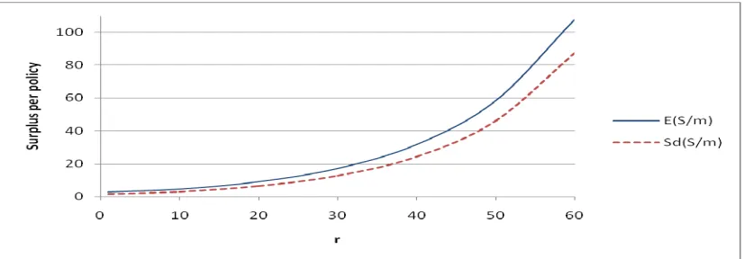
We have carried out 100000 simulations. We evaluate the first 2 moments of the surplus at different dates r and show the results in Figures 1:
Figure 1: Expected Value and variance of the Surplus per policy
We note that, as the valuation date increases, the standard deviation of the surplus increases. In order to understand this, we have to consider that the standard deviation of the surplus is affected by the uncertainty about the cash flows following the premium and by the variance of the interest rate. When r increases, we have to accumulate a greater number of retrospective cash flows for a longer time and discount a smaller number of prospective cash flows for a shorter period. Consequently, the variance of the capitalized cash gains increases and that of the discounted losses decreases. Numerical investigation shows that the first effect prevails over the second one.
6. Distribution Function of Surplus: a stochastic approach
Lysenko and Parker (2007) suggest a recursive method to construct this distribution; the complexity of the product we are considering makes necessary a simulation approach.
One of the objectives of this study is to assess the probability of insolvency, i.e. the probability that it will fall below zero. In order to achieve this purpose, we simulate the evolution of surplus under a mortality and financial stochastic model. Unlike the approach of Lysenko and Parker (2007), we do not approximate the true probability function of surplus by its limiting distribution, which takes into account the investment risk but treats cash flows as given and equal to their expected value. Instead, in order to take account also the longevity risk, we simulate the impact of both financial and mortality factors on retrospective gains and prospective losses.
The financial assumptions are the same as described previously. Also, we need a mortality assumption in order to avoid underestimation or overestimation of the surplus. In this respect, we consider the stochastic model suggested by Cox and Lin (2005) and developed by Ballotta, Esposito and Haberman (2006) and which is described below.
Our calculation is based on the actuarial table used before; however, we estimate the expected value of the number of survivors at age x+t, E[ l(x+t) ], in a stochastic framework. It is possible to prove that l(x+t) is approximately distributed as a normal random variable with mean equal to l(x) tpx and
variance equal to l(x) tpx(1- tpx). However, the recent actuarial literature highlights the fact that the
empirical data show perturbations in survival probabilities due to random shocks. Accordingly, we simulate the survival probabilities adjusted for shocks as follows:
p'x+t = px+t(1−εt) (22)
where εt is the shock in the expected probability at time t. Ballotta, Esposito and Haberman (2006)
assume that εt follows a beta distribution with parameter a and b and the sign of the shocks depends
on the random number k(t) simulated from the uniform distribution U(0,1). In particular, we set:
ε(t) if k(t) < c - ε(t) if k(t) ≥ c
where c is a parameter which depends on the expectation of future mortality trend.
The importance of assigning a random sign to εt is that, in this way, the model captures not only the
long period variations in mortality rates, but also the short period fluctuations due to exceptional circumstances.
We carry out 100000 simulations under different financial and mortality hypotheses. The results are shown in three sections concerning interest rate risk, fund risk and mortality risk.
a. Interest Rate Risk: Numerical Results
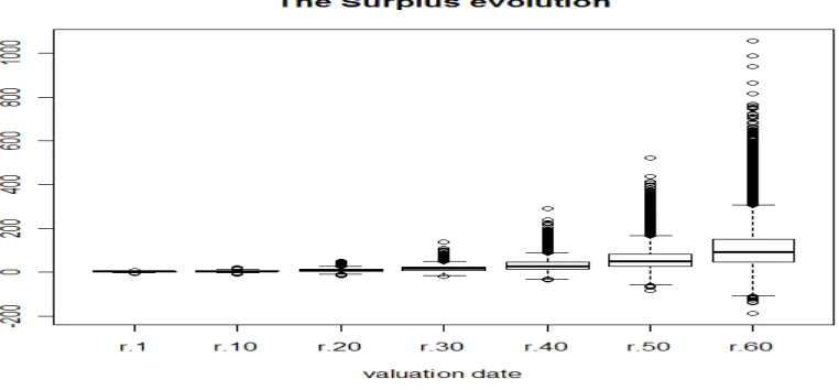
Figure 2: Boxplot of surplus per policy at different valuation dates
S1 S10 S20 S30
Min. :‐7.116 1st Qu.: 1.722 Median : 2.833 Mean : 2.712 3rd Qu.: 3.832 Max. : 7.807
Min. :‐8.306 1st Qu.: 2.615 Median : 4.698 Mean : 4.767 3rd Qu.: 6.828 Max. :20.882
Min. :‐14.194 1st Qu.: 4.637 Median : 8.586 Mean : 9.181 3rd Qu.: 13.063 Max. : 50.022
Min. :‐19.904 1st Qu.: 8.167 Median : 15.590
Mean : 17.209 3rd Qu.: 24.427 Max. :137.021
S40 S50 S60
Min. :‐36.40 1st Qu.: 14.65 Median : 28.19 Mean : 31.80 3rd Qu.: 44.90 Max. :289.38
Min. :‐83.98 1st Qu.: 26.26 Median : 50.89 Mean : 58.50 3rd Qu.: 82.29 Max. :523.09
[image:13.595.217.377.657.746.2]Min. :‐188.80 1st Qu.: 47.16 Median : 92.25 Mean : 107.72 3rd Qu.: 150.80 Max. :1057.44
Table 1 : Summary indices of the surplus distribution per policy at different valuation dates
We want to verify what happens under a different scenario for the force of interest. In particular, we investigate the effect of a reduction in the long mean of the force of interest. We compare the distribution of the Surplus per policy at the valuation date r=1 under the following scenarios:
ScenarioI ScenarioII
δ 0.06 0.04
δ0 0.05 0.05
φ 0.8 0.8
The distributions of surplus are shown and compared in the next figure and table:
Figure 3: The Surplus per policy at r=1 under different scenarios for the forces of interes
As the long rate of return of the assets in which the insurer invests premium decrases, the cumulative distribution of the surplus moves to the left and, consequently, the probability of insolvency increases.
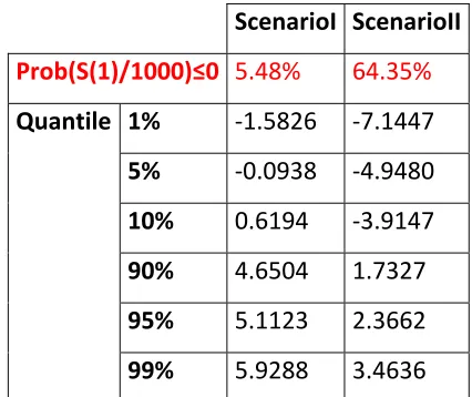
ScenarioI ScenarioII
Prob(S(1)/1000)≤0 5.48% 64.35%
Quantile 1% ‐1.5826 ‐7.1447 5% ‐0.0938 ‐4.9480 10% 0.6194 ‐3.9147 90% 4.6504 1.7327 95% 5.1123 2.3662 99% 5.9288 3.4636
Table 2: Probability of Insolvency and significant percentile of the surplus distribution
This comparison highlights the importance of a correct investment strategy in order to avoid the insolvency. In this case, the insurer has to invest the collected premiums into assets with a long mean of the rate of return equal to 0.06 in order to have a positive surplus since the first year and not ask other money to shareholders. We note that if the insurer invests the premiums into assets that in mean yield a return equal to the guaranteed rate on GMDB the probability of insolvency at r=1 is 64.35%.
[image:14.595.190.403.422.601.2]b. Fund Risk: Numerical Results
In this section, we study the effect of shifts in the distributions of fund value. As we wish to produce a sensitivity analysis, we fix the hypothesis concerning the interest rate distribution according the parameters used in section 5 and change those concerning the fund. In particular, we compare the surplus distributions under the following four scenarios:
Scenario I II III IV µ-η 0.06 0.06 0.06 0.05
σ2 0.03 0.04 0.03 0.03
g 0.04 0.04 0.05 0.04
The results are summarized in the next table:
Scenario I Scenario II Scenario III Scenario IV
Min. : 19.904 1st Qu. : 8.167 Median : 15.590 Mean : 17.209 3rd Qu. : 24.427 Max. :137.021
Min. :‐40.943 1st Qu.: 8.013 Median : 15.434 Mean : 17.022 3rd Qu.: 24.251 Max.: 136.487
Min. :‐20.354 1st Qu.: 7.611 Median : 15.019
Mean : 16.642 3rd Qu.: 23.849 Max. : 136.568
Min. : ‐14.547 1st Qu.: 9.485
[image:15.595.175.419.169.236.2]Median : 16.901 Mean : 18.532 3rd Qu.: 25.726 Max. : 138.754
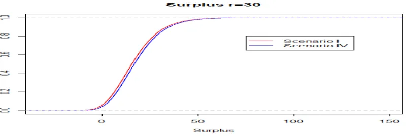
Table 3 : Summary indices of the surplus distribution per policy under different scenarios
[image:15.595.93.493.532.666.2]As expected, as the volatility of the fund increases the variance of the surplus increases and as the guaranteed rate increases the mean of the surplus distribution decreases. Moreover, as the drift of the fund process decreases, the distribution of the surplus moves on the right, as shown in Figure 4, because the amounts of death benefits paid decrease.
c.Mortality Risk: Numerical Results
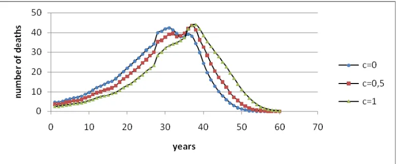
In this section, we study the effect of shifts in the parameters of stochastic mortality model. In the same manner as the previous sections, we aim to produce a sensitivity analysis, and so we fix the hypothesis concerning the interest rate and the fund evolution as in section 5 and change the mortality table. In particular, we use the mortality model described and set a=0.5 and b=4.5. we evaluate the surplus per policy at r=30. We consider three cases for the value of c: c = 0, 0.5, 1. In the first case, there will be improvements in life expectancy at every date; in other words, all of the shocks are expected to be positive. Conversely, in the second case further improvements of an already high expectancy of life are impossible and all shocks are expected to be negative.
[image:16.595.104.497.338.500.2]Under the hypothesis c=1, the outflows linked to annuities increase and, under the hypothesis c=0, they decrease. In Figure 16, we show the cdf of the number of deaths that occur in each year under the hypotheses c=0, c=0,5 and c=1. Under the hypothesis c=0, the pdf of the number of deaths is translated to the left and it has a fatter left tail and a less fat right tail than the other two curves. On the contrary, if c=1 the pdf of the number of deaths is translated to the right and it has a less fat left tail and a fatter right tail than the other two curves
Figure 5: Pdf of the number of deaths under the hypotheses c=0, c=0,5 and c=12.
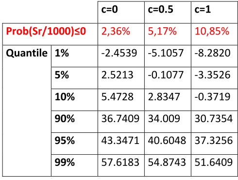
As c increases, the outflows linked to the annuity increase; moreover, the payments related to the GMDB option increase too, because they are rolled over and they are linked to a fund value that increases with time. Consequently, the cumulative distribution of the surplus moves on the left and the probability of insolvency increases. These results are illustrated in Figure 6 and Table 4.
2 Figure 5 shows an unusual feature: each curve has two modes. The 2‐modal feature can be found also in a recent
Figure 6: the distiubution of the Surplus per policy under different mortality hypothesis
c=0 c=0.5 c=1
Prob(Sr/1000)≤0 2,36% 5,17% 10,85%
Quantile 1% ‐2.4539 ‐5.1057 ‐8.2820 5% 2.5213 ‐0.1077 ‐3.3526 10% 5.4728 2.8347 ‐0.3719 90% 36.7409 34.009 30.7354
95% 43.3471 40.6048 37.3256
99% 57.6183 54.8743 51.6409
Table 4: Probability of Insolvency and significant percentile of the surplus distribution under different mortality hypothesis.
7. Conclusions
[image:17.595.174.419.329.514.2]expenses and lapse options are not considered; and further random lifetimes and rates of return are assumed to be independent. These are limitations of our framework and in subsequent work the model will be improved by introducing a more complex and realistic model structure and assumptions.
Despite the above limitations, we believe that the paper is useful in enhancing an insurer’s understanding of the stochastic behaviour underlying a Variable Annuity product with a GMDB option and that it provides the first study of the surplus in respect of this recently developed insurance product. Indeed, up to this time, the literature has offered only pricing models for GMDB, but has not studied the evolution of cash flows. We deem this consideration is important in the perspective of the liquidity and insolvency risk management. We have considered both financial and mortality risk and have outlined a comprehensive description of the interaction of different risk factors on the GMDB value.As general rule, if a death benefit is added to an annuity, there is a sort of “mortality natural hedging effect”, i.e. the impact of longevity risk is reduced because the annuity is paid for a longer period but the actual value of the death benefit decreases. The GMDB options can represent an exception to this rule; in section 6.3 we have shown that as the estimated life extends the outflows linked to the annuity increase and at the same time the payments related to the GMDB option increase too, because they are rolled over and they are linked to a fund value that increases with time. Therefore, under the hypothesis of a growing fund, the effect of “natural hedging” is nullified. Hence, it is not sufficient to study the impact of each risk factor on the GMDB value, but it is necessary to examine their interaction.
In the paper, numerical examples show a significant impact of the interest, fund and mortality risks on the surplus distribution, insomuch as the insolvency probability increases considerably in many cases. With regard to this point, an advantage of the model used is that it allows an ex ante assessment of the insurer’s solvency throughout the duration of contract. Consequently, a change to the design of the product can be made, and, in particular, the premium can be modified according to the forecasts of mortality probabilities, interest rate and fund evolution. Moreover, the model enables us to determine the premium that leads to a required probability of insolvency, and so it can be used for an evaluation of the adequacy of solvency, which is consistent with recent regulatory changes.
References
Ballotta L., Esposito G., Haberman S. (2006). Modelling the Fair Value of Annuities Contracts: The Impact of Interest Rate Risk and Mortality Risk. Actuarial Research Paper No.176, Cass Business School.
Ballotta L., Haberman S. (2006), The fair valuation problem of guaranteed annuity options: The stochastic mortality environment case, Insurance: Mathematics and Economics 38, 195-214
Bellhouse D.R., Panjer H.H. (1981). Stochastic modeling of interest rates with applications to life contingiencies. Journal of Risk and Insurance, 48(4), 628-637
Cairns A.J.G., Parker G. (1997). Stochastic pension fund modeling. Insurance: Mathematics and Economics, 21, 43-79
Coleman T.F., Li Y., Patron M. (2006). Hedging guarantees in variable annuities under both equity and interest rate risks. Insurance: Mathematics and Economics 38, 215-228
Coppola M., Di Lorenzo E., Sibillo M. (2003). Stochastic analysis in life office management: applications to large annuity portfolios. Applied Stochastic Models in Business and Industry 19, 31-42.
Cox S.H., Lin Y. (2005). Securitization of mortality risk in life annuities. The Journal of Risk and Insurance 72, 227-252
Dahl M. (2004). Stochastic mortality in life insurance: market reserves and mortality- linked insurance contracts. Insurance: Mathematics and Economics 35, 113-136
Haberman S., Piscopo G. (2008). Mortality Risk and the Valuation of Annuities with Guaranteed Minimum Death Benefit Options: Application to the Italian Population. Actuarial Research Paper No. 187, Cass Business School.
Hoedemakers T., Darkiewicz G., Goovaerts M. (2005). Approximations for life annuity contracts in a stochastic financial environment. Insurance: Mathematics and Economics 37, 239-269.
Ledlie M.C., Corry D.P., Finkelstein G.S., Ritchie A.J., Su K., Wilson D.C.E (2008). Variable annuities. Presented to the Institute of Actuaries.
Lysenko N., Parker G. (2007). Stochastic Analysis of Life Insurance Surplus. Presented to the 2007 AFIR Colloquium.
Marceau E., Gaillardetz P. (1999). On life insurance reserves in a stochastic mortality and interest rates environment. Insurance: Mathematics and Economics, 25, 261-280.
Milevsky M., Posner S.E. (2001). The Titanic Option: Valuation of the Guaranteed Minimum Death Benefit in Variable Annuities and Mutual Funds. The Journal of Risk and Insurance 68, 1, 91-126.
Milevsky M., Salisbury T.S. (2002), The Real Option to Lapse and the Valuation of Death-Protected Investments. Working Paper York University and the Fields Institute, Toronto.
Milevsky M.A., Promislow S.D. (2001), Mortality derivatives and the option to annuities. Insurance: Mathematics and Economics 29, 299-318
Parker G. (1996). A portfolio of endowment policies and its limiting distribution. ASTIN Bulletin, 26, 25-33.
APPENDIX A
Let T be the future lifetime random variable expressed in continuous time, Fx(t) be its cdf and fx(t)
be its pdf; therefore, for an individual aged x the probability of death before time t is
Fx(t) = P ( T ≤ t ) = 1- tpx = 1- exp
⎭
⎬
⎫
⎩
⎨
⎧
+
−
∫
tx
s
ds
0
)
(
ς
where ζ denotes the force of mortality.
Let Vt be the account value at time t linked to fund value. Following standard assumptions in the
literature, we model the evolution of the account as:
where Wt is a standard Brownian motion, µ is the drift rate, η is the charge paid for the GMDB
option.
The risk neutral process for Vt is:
Q t t t
t
r
V
dt
V
dW
dV
=
(
−
η
)
+
σ
where r is the risk free rate and WtQ is a Brownian motion under a new Girsanov transformed
measure Q. The solution of the SDE is:
Q t W t r
t
V
e
V
=
0 ( −η−σ2/2) +σ .Now we describe the GMDB payoff. At the random date of death τ the beneficiary will receive
τ τ τ τ
τ τ
τ e V V e V e V V
Dp =max( g 0, )= g max( 0− −g ,0)+ where g is the guaranteed rate.
The value of the GMDB option at τ is the sum of the fund value and a put option whose strike price is the initial value V0, with an underlying asset Vτ discounted by the guaranteed growth rate g.
Since the maturity is stochastic and τ and Vτ are independent, the present value of GMDB is given
by the expectations under τ and Vτ:
{
}
{
E e D t}
E
D0p = t Q −rτ τpτ=
If we fixed the date τ, we have at τ an European Option, whose actual value can be calculated with Black and Scholes formula. Therefore, the previous formula can be interpreted as a decomposition of the actual value of GMDB in the actual value of a continuous sequence of European put option. Substituting the expression of Dp
τ
t t t
t
V
dt
V
dW
{
}
{
E e V e V e V t}
E
D0p = t Q −(r−g)τ max( 0− −gτ τ,0)+ −rτ ττ =
We can observe that
{
e
V
}
e
V
0E
Q −rτ τ=
−ητsince we have assumed that Vt is a geometric Brownian motion with drift equal to r-δ and so its
expected value is:
{ }
( )0 )
0
(
V
e
V
E
Q τ=
r−ητConsequently:
{
}
{
}
{
}
{
E
e
V
e
V
e
t
}
E
t
V
e
V
e
V
e
E
E
D
g g r Q t r g g r Q t p=
+
−
=
=
=
+
−
=
− − − − − − − −τ
τ
ητ τ τ τ τ τ τ τ τ)
0
,
max(
)
0
,
max(
0 ) ( 0 ) ( 0We observe that for a fixed date T
{
}
[
]
(
)
(
)
[
T]
T T T r T T gT T g r Q
e
T
r
BS
V
e
d
N
e
d
N
e
V
e
V
e
V
e
E
η η η ησ
η
− − − − − − − −+
≡
≡
+
−
−
−
≡
≡
+
−
)
,
,
,
~
)
(
)
(
)
0
,
max(
0 1 2 ~ 0 0 ) ( whereσ
σ
η
T
r
d
/
2
)
~
(
21
+
−
=
; d2 =d1−σ T ; r~=r−g; N(.) is the cumulative probabilityfunction for a random variable normally distributed.
If we consider both the expectations:
(
)
[
BS
r
t
e
]
dt
V
t
f
D
t x xp
=
ω−η
σ
+
−δ∫
(
)
0~
,
,
,
)
0 0
In the discrete case we have:
[
t]
x t t x x t p
e
t
r
BS
V
q
p
D
δ ωσ
η
− − = ++
=
∑
(
~
,
,
.
)
1 0 0for a policyholder aged x at inception of the contract.
APPENDIX B
The variance of the cash flows (both retrospective or prospective) is given by the following formula:
[ ]
FCrj R Var[ ]
j Var[
Gj j]
RCov[
j Gj j]
Var = 2 α + δ +2 α , δ
where
•
[
]
[ ] [ ]
2 2(
[ ]
)
2(
[ ]
)
2j j
j j j
j EG E EG E
G
Var δ = δ − δ ;
• Cov
[
αj,Gjδj] [ ] [
=EGj Covαj,δj]
in fact
[
] [
] [ ] [
] [ ] [
] [ ] [ ] [ ]
[ ] [
j{
j j] [ ] [ ]
j j}
[ ] [
j j j]
j j j j j j j j j j j j j j j Cov G E E E E G E E G E E E G E G E E G E G Cov δ α δ α δ α δ α δ α δ α δ α δ α , , = − = = − = − = ;
The covariance of the cash flows is:
[
FCk(r),FC(jr)]
=Cov
[
k j]
Cov[
Gk k Gj j]
RCov[
k Gj j]
RCov[
j Gk k]
Cov
R2 α ,α + δ , δ + α , δ + α , δ =
where
• Cov
[
Gkδk,Gjδj] [
=EGkδkGjδj]
−E[
Gkδk]
E[
Gjδj]
=[
] [ ]
[ ] [ ]
[ ] [ ]
[ ]
[ ] [ ]
[ ] [ ]
[ ] [ ]
[ ]
[ ] [ ]
{
[ ]
[ ]
}
[ ]
k[ ] [
j k j]
j k j k j k j j k k j k j k j j k k j k j k Cov G E G E E E E G E G E E G E E G E E G E G E E G E E G E E G G E δ δ δ δ δ δ δ δ δ δ δ δ δ δ , = = − = − = = − =
• Cov
[
αk,Gjδj] [ ] [
=EGj Covαk,δj]
• Cov
[
αj,Gkδk]
=E[ ]
Gk Cov[
αj,δk]
[ ]
[
]
(
)
⎪ ⎪ ⎭ ⎪⎪ ⎬ ⎫ ⎪ ⎪ ⎩ ⎪⎪ ⎨ ⎧ + = ⎥ ⎥ ⎦ ⎤ ⎢ ⎢ ⎣ ⎡ =∑
∑
∑ ∑
= ≠ = = = n j n j k k r k I r k r j I r j n j r j I r j n j r j I r jr VarFC e CovFC e FCe
m m e FC Var m S Var 0 0 ) , ( ) , ( 0 ) , ( 2 0 ) , ( , 1 / where
•
[
r I(j,r)]
=je
FC Var
[
] [
−{
]
}
=[ ] [
]
−[ ]
[
]
= = 2 ( , )2 ( , ) 2 2 ( , )2 2 I(j,r) 2j r j I j r j I r j r j I
je EFC e EFC Ee EFC Ee
FC
E
•
[
( , ), r I(k,r)]
=k r j I r
je FC e
FC Cov
[
] [ ] [
] [ ] [
]
[
] [
] [ ] [
] [ ] [
]
[
] [
{
( , ) ( , )] [
( , )] [
( ,)]
}
[ ] [
( ,)] [ ] [
( , )]
) , ( ) , ( ) , ( ) , ( ) , ( ) , ( ) , ( ) , (, r I kr
FACULTY OF ACTUARIAL SCIENCE AND INSURANCE
Actuarial Research Papers since 2001
Report Number
Date Publication Title Author
160. January 2005 Mortality Reduction Factors Incorporating Cohort Effects.
ISBN 1 90161584 7
Arthur E. Renshaw Steven Haberman
161. February 2005 The Management of De-Cumulation Risks in a Defined Contribution Environment. ISBN 1 901615 85 5.
Russell J. Gerrard Steven Haberman Elena Vigna
162. May 2005 The IASB Insurance Project for Life Insurance Contracts: Impart on Reserving Methods and Solvency
Requirements. ISBN 1-901615 86 3.
Laura Ballotta Giorgia Esposito Steven Haberman
163. September 2005 Asymptotic and Numerical Analysis of the Optimal Investment Strategy for an Insurer. ISBN 1-901615-88-X
Paul Emms Steven Haberman
164. October 2005. Modelling the Joint Distribution of Competing Risks Survival Times using Copula Functions. I SBN 1-901615-89-8
Vladimir Kaishev Dimitrina S, Dimitrova Steven Haberman
165. November 2005.
Excess of Loss Reinsurance Under Joint Survival Optimality. ISBN1-901615-90-1
Vladimir K. Kaishev Dimitrina S. Dimitrova
166. November 2005.
Lee-Carter Goes Risk-Neutral. An Application to the Italian Annuity Market.
ISBN 1-901615-91-X
Enrico Biffis Michel Denuit
167. November 2005 Lee-Carter Mortality Forecasting: Application to the Italian Population. ISBN 1-901615-93-6
Steven Haberman Maria Russolillo
168. February 2006 The Probationary Period as a Screening Device: Competitive Markets. ISBN 1-901615-95-2
Jaap Spreeuw Martin Karlsson
169. February 2006 Types of Dependence and Time-dependent Association between Two Lifetimes in Single Parameter Copula Models. ISBN 1-901615-96-0
Jaap Spreeuw
170. April 2006 Modelling Stochastic Bivariate Mortality ISBN 1-901615-97-9
Elisa Luciano Jaap Spreeuw Elena Vigna.
171. February 2006 Optimal Strategies for Pricing General Insurance. ISBN 1901615-98-7
Paul Emms Steve Haberman Irene Savoulli
172. February 2006 Dynamic Pricing of General Insurance in a Competitive Market. ISBN1-901615-99-5
Paul Emms
173. February 2006 Pricing General Insurance with Constraints. ISBN 1-905752-00-8
Paul Emms
Report Number
Date Publication Title Author
175. December 2006 Pricing and Capital Requirements for With Profit Contracts: Modelling Considerations. ISBN 1-905752-04-0
Laura Ballotta
176. December 2006 Modelling the Fair Value of Annuities Contracts: The Impact of Interest Rate Risk and Mortality Risk. ISBN 1-905752-05-9
Laura Ballotta Giorgia Esposito Steven Haberman
177. December 2006 Using Queuing Theory to Analyse Completion Times in Accident and Emergency Departments in the Light of the Government 4-hour Target. ISBN 978-1-905752-06-5
Les Mayhew David Smith
178. April 2007 In Sickness and in Health? Dynamics of Health and Cohabitation in the United Kingdom. ISBN 978-1-905752-07-2
Martin Karlsson Les Mayhew Ben Rickayzen
179. April 2007 GeD Spline Estimation of Multivariate Archimedean Copulas. ISBN 978-1-905752-08-9
Dimitrina Dimitrova Vladimir Kaishev Spiridon Penev
180. May 2007 An Analysis of Disability-linked Annuities. ISBN 978-1-905752-09-6
Ben Rickayzen
181. May 2007 On Simulation-based Approaches to Risk Measurement in Mortality with Specific Reference to Poisson lee-Carter Modelling. ISBN 978-1-905752-10-2
Arthur Renshaw Steven Haberman
182. July 2007 High Dimensional Modelling and Simulation with Asymmetric Normal Mixtures. ISBN 978-1-905752-11-9
Andreas Tsanakas Andrew Smith
183. August 2007 Intertemporal Dynamic Asset Allocation for Defined Contribution Pension Schemes. ISBN 978-1-905752-12-6
David Blake Douglas Wright Yumeng Zhang
184. October 2007 To split or not to split: Capital allocation with convex risk measures. ISBN 978-1-905752-13-3
Andreas Tsanakas
185. April 2008 On Some Mixture Distribution and Their Extreme Behaviour. ISBN 978-1-905752-14-0
Vladimir Kaishev Jae Hoon Jho
186. October 2008 Optimal Funding and Investment Strategies in Defined Contribution Pension Plans under Epstein-Zin Utility. ISBN 978-1-905752-15-7
David Blake Douglas Wright Yumeng Zhang
187. May 2008 Mortality Risk and the Valuation of Annuities with
Guaranteed Minimum Death Benefit Options: Application to the Italian Population. ISBN 978-1-905752-16-4
Steven Haberman Gabriella Piscopo
188. January 2009 The Market Potential for Privately Financed Long Term Care Products in the UK. ISBN 978-1-905752-19-5
Leslie Mayhew
189. June 2009 Whither Human Survival and Longevity or the Shape of things to Come. ISBN 978-1-905752-21-8
Leslie Mayhew David Smith
190 October 2009 ilc: A Collection of R Functions for Fitting a Class of Lee Carter Mortality Models using Iterative fitting Algorithms* ISBN 978-1-905752-22-5
Zoltan Butt Steven Haberman
191. October 2009 Decomposition of Disease and Disability Life Expectancies in England, 1992-2004. ISBN 978-1-905752-23-2
Report Number
Date Publication Title Author
192. October 2009 Exploration of a Novel Bootstrap Technique for Estimating the Distribution of Outstanding Claims Reserves in General Insurance. ISBN 978-1-905752-24-9
Robert Cowell
193. January 2010 Surplus Analysis for Variable Annuities with a GMDB Option. ISBN 978-1-905752-25-6
Steven Haberman Gabriella Piscopo
Statistical Research Papers
1. December 1995. Some Results on the Derivatives of Matrix Functions. ISBN 1 874 770 83 2
P. Sebastiani
2. March 1996 Coherent Criteria for Optimal Experimental Design.
ISBN 1 874 770 86 7
A.P. Dawid P. Sebastiani
3. March 1996 Maximum Entropy Sampling and Optimal Bayesian
Experimental Design. ISBN 1 874 770 87 5
P. Sebastiani H.P. Wynn
4. May 1996 A Note on D-optimal Designs for a Logistic Regression Model. ISBN 1 874 770 92 1
P. Sebastiani R. Settimi
5. August 1996 First-order Optimal Designs for Non Linear Models.
ISBN 1 874 770 95 6
P. Sebastiani R. Settimi
6. September 1996 A Business Process Approach to Maintenance: Measurement, Decision and Control. ISBN 1 874 770 96 4
Martin J. Newby
7. September 1996.
Moments and Generating Functions for the Absorption Distribution and its Negative Binomial Analogue.
ISBN 1 874 770 97 2
Martin J. Newby
8. November 1996. Mixture Reduction via Predictive Scores. ISBN 1 874 770 98 0 Robert G. Cowell.
9. March 1997. Robust Parameter Learning in Bayesian Networks with Missing Data. ISBN 1 901615 00 6
P.Sebastiani M. Ramoni
10. March 1997. Guidelines for Corrective Replacement Based on Low Stochastic Structure Assumptions. ISBN 1 901615 01 4.
M.J. Newby F.P.A. Coolen
11. March 1997 Approximations for the Absorption Distribution and its Negative Binomial Analogue. ISBN 1 901615 02 2
Martin J. Newby
12. June 1997 The Use of Exogenous Knowledge to Learn Bayesian
Networks from Incomplete Databases. ISBN 1 901615 10 3
M. Ramoni P. Sebastiani
13. June 1997 Learning Bayesian Networks from Incomplete Databases.
ISBN 1 901615 11 1
M. Ramoni P.Sebastiani
14. June 1997 Risk Based Optimal Designs. ISBN 1 901615 13 8 P.Sebastiani
H.P. Wynn
15. June 1997. Sampling without Replacement in Junction Trees.
ISBN 1 901615 14 6
Robert G. Cowell
16. July 1997 Optimal Overhaul Intervals with Imperfect Inspection and Repair. ISBN 1 901615 15 4
Report Number
Date Publication Title Author
18. November 1997. A Characterisation of Phase Type Distributions.
ISBN 1 901615 18 9
Linda C. Wolstenholme
19. December 1997 A Comparison of Models for Probability of Detection (POD) Curves. ISBN 1 901615 21 9
Wolstenholme L.C
20. February 1999. Parameter Learning from Incomplete Data Using Maximum Entropy I: Principles. ISBN 1 901615 37 5
Robert G. Cowell
21. November 1999 Parameter Learning from Incomplete Data Using Maximum Entropy II: Application to Bayesian Networks. ISBN 1 901615 40 5
Robert G. Cowell
22. March 2001 FINEX : Forensic Identification by Network Expert Systems. ISBN 1 901615 60X
Robert G.Cowell
23. March 2001. Wren Learning Bayesian Networks from Data, using Conditional Independence Tests is Equivalant to a Scoring Metric ISBN 1 901615 61 8
Robert G Cowell
24. August 2004 Automatic, Computer Aided Geometric Design of Free-Knot, Regression Splines. ISBN 1-901615-81-2
Vladimir K Kaishev, Dimitrina S.Dimitrova, Steven Haberman Richard J. Verrall
25. December 2004 Identification and Separation of DNA Mixtures Using Peak Area Information. ISBN 1-901615-82-0
R.G.Cowell S.L.Lauritzen J Mortera,
26. November 2005. The Quest for a Donor : Probability Based Methods Offer Help. ISBN 1-90161592-8
P.F.Mostad T. Egeland., R.G. Cowell V. Bosnes Ø. Braaten
27. February 2006 Identification and Separation of DNA Mixtures Using Peak Area Information. (Updated Version of Research Report Number 25). ISBN 1-901615-94-4
R.G.Cowell S.L.Lauritzen J Mortera,
28. October 2006 Geometrically Designed, Variable Knot Regression Splines : Asymptotics and Inference. ISBN 1-905752-02-4
Vladimir K Kaishev Dimitrina S.Dimitrova Steven Haberman Richard J. Verrall
29. October 2006 Geometrically Designed, Variable Knot Regression Splines : Variation Diminishing Optimality of Knots.
ISBN 1-905752-03-2
Vladimir K Kaishev Dimitrina S.Dimitrova Steven Haberman Richard J. Verrall
30. November 2008 Scheduling Reentrant Jobs on Parallel Machines with a Remote Server. ISBN 978-1-905752-18-8
Konstantin Chakhlevitch Celia Glass
Faculty of Actuarial Science and
Insurance
Cass Business School
Copyright 2010 © Faculty of Actuarial Science and Insurance, Cass Business School