Validation of Tools to Accelerate High-Speed CFD
Simulations Using OpenFOAM
Daniel E. R. Espinoza
∗, Thomas J. Scanlon
†and Richard E. Brown
‡Centre for Future Air-Space Transportation Technology,
University of Strathclyde, Glasgow, G1 1XJ, United Kingdom
Local time stepping (LTS) and adaptive mesh refinement (AMR) have been implemented into rhoCentralFoam, a compressible solver within the open source computational fluid dynamics (CFD) code OpenFOAM. The LTS solver has been validated using a compressible Couette channel with heat transfer and a supersonic flat plate. An excellent concurrence is found for these cases in comparison with the solutions with the obtained results being, respectively, 2.56 and 8.96 times faster compared to the unmodified solver. The AMR solver was employed to simulate hypersonic flow over a 30◦wedge, and the Sod shock tube test case, and has also achieved satisfactory agreement with the analytical solutions. These results highlight the potentially significant computational cost savings that may be achieved when solving high-speed, compressible flows using this approach.
Nomenclature
F Flux array
S Source terms array
W Conserved variables array
~v Velocity vector, m/s
a Acceleration factor
c Courant number
H Height of the channel, m
k Thermal conductivity, W/(m·K)
L Length of the shock tube
M Mach number
p Pressure, Pa
Re Reynolds number
T Temperature, K
t Time, s
U Flow speed in the x direction, m/s
x Horizontal coordinate, m
y Vertical coordinate, m
AMR Adaptive Mesh Refinement
CFD Computational Fluid Dynamics DPLR Data-Parallel Line Relaxation
LAURA Langley Aerothermodynamic Upwind Re-laxation Algorithm
LTS Local time stepping
OpenFOAM Open Source Field Operation And Ma-nipulation
TVD Total Variation Diminishing
Subscripts
∞ Upstream conditions
BW Bottom wall
l Initial conditions at left half of shock tube
max Maximum
r Initial conditions at right half of shock tube
T W Top wall
Symbols
∆t Time-step, s
µ Dynamic viscosity, Pa·s
∇ Gradient operator
ρ Density, kg/m3
I.
Introduction
To be able to satisfactorily capture the essential flow features in the simulation of hypersonic flows, good practice dictates that a specific set of procedures should be followed. These include the categorisation of the correct physics (e.g. non-equilibrium effects,1 modelling of turbulence2) as well as the selection of the most
appropriate solution methodologies to capture the essential physics (e.g. shock-capturing and shock-fitting approaches,3 choice of TVD schemes4,5). Whereas a significant amount of research has been dedicated to
these areas, this paper focuses on how the spatial and temporal resolution of calculations may be improved in order to achieve satisfactory numerical results with an accompanying reduction in computational expense.
With regard to spatial resolution, a computational mesh that attempts to follow the shock structure is an essential feature of the solution methodology. In terms of the cell shape, a tetrahedral mesh can be created more quickly than a structured one and delivers greater flexibility, in particular for complex geometries. Poor predictions of heat transfer can result6 however, and, for this reason, standard practice for unstructured meshes is to attempt to have prismatic cells aligned with solid surfaces and the shock wave itself.7 This alignment of the grid with the shock wave is particularly important in order to avoid significant
fluctuations occurring in the prediction of the stagnation point heat flux.8 In addition, a sufficient degree of
cell refinement is required near the shock wave simply in order to properly capture the spatial variation in the flow properties there.9 In this paper we present a mesh refinement strategy which significantly improves
the capturing of spatial gradients in the flow field.
The rate of temporal advance of the computation must also be such that the numerical stability and accuracy of the calculation are preserved. We present a time-acceleration technique which shows potential to greatly accelerate the computation of the initial transient within the computation and hence the rate of convergence of the calculation towards its steady state.
Some well-known hypersonic codes (e.g. LAURA10and DPLR11) contain features to deal with the spatial and temporal issues described above. Although the open source computational fluid dynamics code used in this paper, OpenFOAM,12 does have such capabilities, the libraries that include these features have yet to be included in its high-speed compressible solvers. The objective of this paper is to incorporate local time stepping (LTS) and adaptive mesh refinement (AMR) into the OpenFOAM high-speed compressible solver
rhoCentralFoam, and to validate the results of computations using this new approach against appropriate
analytical solutions or experimental data.
II.
Methodology
OpenFOAM is an open source computational fluid dynamics (CFD) software package consisting of a set of flexible C++ modules to resolve complex fluid flows. The package includes tools for meshing and pre-and post-processing, as well as solvers for both incompressible pre-and compressible flows.12
Amongst the compressible solvers that are available in OpenFOAM, rhoCentralFoam13has been chosen
for the simulations presented in this work, largely because of its satisfactory performance in previously-conducted high-speed compressible flow simulations.13,14 rhoCentralFoam is an unsteady, compressible
solver, that uses semi-discrete, non-staggered, Godunov-type central15and upwind-central16schemes. These
schemes both avoid the explicit need for a Riemann solver, resulting in a numerical approach that is both simple and efficient.16
II.A. Local time stepping
allowed for any cell. LTS allows each cell to advance in time at their own time-step.
While the Navier-Stokes equations have the form
∂W
∂t +∇ ·F=S (1)
whereWrepresents the conserved variables,Fthe fluxes,Sthe source terms,tthe time, and∇the gradient operator, the LTS technique solves the equation
1 a
∂W
∂t +∇ ·F=S (2)
whereais an acceleration factor that depends onW.
If the solution is steady, then the time derivative is exactly zero, and so a solution to Equation (2) is also a solution of Equation (1), independent of the value ofa.
In the LTS procedure that has been implemented into OpenFOAM, the time derivative is modelled using an Euler scheme. Based on similar implementations in the OpenFOAM solver LTSInterFoam and those found in Ref. 17, the time-step ∆tfor each cell is selected individually as the minimum between the global, user-defined maximum time-step ∆tmax, and the time-step that is determined by the maximum allowable
Courant numbercmax within the flow. In other words
∆t= min (∆tmax,∆t(cmax)) (3)
In practice, the field ∆t calculated using this approach is first smoothed spatially before being applied to the calculation of the LTS solution in each computational cell.
II.B. Adaptive Mesh Refinement
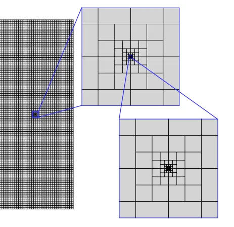
Adaptive mesh refinement (AMR) is a technique that is used to modify an existing mesh so as to improve its resolution of the flow properties in regions of interest, and thus to capture the flow with enhanced accu-racy without an excessive increase in computational effort. The advantage of implementing this technique within OpenFOAM is that it allows the details of the flow near shocks to be captured without the need for an excessively fine mesh throughout the entire computational domain. Based on the implementations within the OpenFOAM solversinterDyMFoam andrhoCentralDyMFoam, the computational mesh is refined or coarsened locally during the computation in order to adapt to the spatial gradients within the flow prop-erties. The approach uses a tree structure, and the maximum coarsening that can be obtained is equivalent to the cell density of the base mesh. When refining the mesh, the algorithm splits each hexahedral cell in two along each coordinate direction to generate eight new cells from the original parent cell. Figure 1 shows the refinement algorithm that is used by the AMR procedure and Figure2 illustrates an example of a parent-child tree that could be obtained when a cell is split using this procedure.
II.C. Test cases
The following test cases have been used to validate the LTS and AMR algorithms as implemented within
rhoCentralFoam.
Figure 1. Flow chart for the refinement algorithm
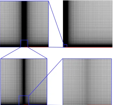
[image:4.612.246.366.71.399.2] [image:4.612.140.473.461.684.2]domain is illustrated in Figure3. The base cell size was set to 0.01 m×0.01 m. Four cells were refined at the centre of the channel, then the four cells at the centre of the group of refined cells, and so on until 11 levels of refinement were achieved. The finest cell has a size of≈4.88µm×4.88µm, as can be seen in Figure3.
The fluid within the channel is air, and the initial and boundary conditions are set to
~v(t= 0) = 0m/s T(t= 0) = 200K p(t= 0) = 100P a
UT W = 200m/s TT W = 400K
UBW = 0m/s TBW = 200K
where~vrepresents the velocity vector,T the temperature,pthe pressure,U the flow speed in thex-direction, and the subscriptsT W andBW refer to the top and bottom walls of the channel respectively.
The maximum allowable courant number in the flow was set to 0.2 and the maximum allowable time-step to 1×10⁻³ s.
For the supersonic flat plate,18 the length of the plate within the domain was 0.1 m, with the domain
extending 5×10⁻³ m behind the plate. Figure4shows the 2-Dimensional computational domain, with the
flate plate in red, and consecutive zoom to be able to appreciate the mesh in detail. The smallest cells, at the leading edge of the plate, have a size of 1µm×1µm, whereas the coarsest cell, at the top right corner, has a size of≈2.8 mm×2.8 mm.
The fluid within the domain is air, and the initial and boundary conditions are set so to match the Reynolds (Re) and Mach (M) numbers to those is Ref. 18, as well as the flat plate/upstream temperature ratio (that is, Re = 500, M∞ = 2 and TTW∞ = 2). Setting the upstream temperature to 300K, and using 0.01m as the reference length to calculate the Reynolds number, the initial and boundary conditions result in:
U(t= 0) = 694.55m/s T(t= 0) = 300K p(t= 0) = 114.46P a
U∞= 694.55m/s T∞= 300K p∞= 114.46P a
II.C.2. AMR
A first verification of the implementation of the AMR technique within rhoCentralFoam was conducted by modelling the inviscid flow at Mach 5 over a two-dimensional 30◦wedge. The initial mesh can be seen in Figure5.
Figure 5. Initial mesh for the supersonic wedge test case
The fluid used for this simulation has been set up so to resolve the non-dimensional problem. As such, the initial and boundary conditions are
~
v(t= 0) = 0 M∞= 5
T(t= 0) = 1 T∞= 1
p(t= 0) = 1 p∞= 1
No-slip, adiabatic wall boundaries are assumed.
Mesh refinement was instigated whenk∇Mk>1, and coarsening whenk∇Mk<1. A million time-steps were executed between each mesh update.
In addition, the Sod shock tube test case19 was used to study the suitability of the AMR technique for
transient simulations. The initial mesh can be seen in Figure6.
Figure 6. Initial mesh for the shock tube test case
[image:8.612.110.502.120.363.2] [image:8.612.67.543.612.663.2]the initial conditions are
u(x/L <0, t= 0) =ul= 0 u(x/L >0, t= 0) =ur= 0
p(x/L <0, t= 0) =pl= 1 p(x/L >0, t= 0) =pr= 0.1
ρ(x/L <0, t= 0) =ρl= 1 ρ(x/L >0, t= 0) =ρr= 0.125
whereL represents the length of the shock tube,ρthe density of the fluid, and the subscriptsl andrrefer to the left and right half of the shock tube respectively.
Two different refinement/coarsening criteria were compared. For the first criterion, mesh refinement was
instigated when ∇p p
>1, and coarsening when ∇p p
<0.5. For the second, the mesh was refined when ∇ρ ρ
> 1 and coarsened when ∇ρ ρ
< 0.5. For both cases, five time-steps were executed between each
mesh update.
III.
Results and discussion
III.A. LTS
III.A.1. Couette flow
The figures presented below show the flow properties along the vertical centreline through the Couette channel and are compared with the analytical solution for the flow, namely:
T(y) =TBW + (TT W −TBW)
y H +
µUT W2 2k
y H
1− y
H
(4)
U(y) =UT W
y
H (5)
V(y) = 0m/s (6)
p(y) =constant (7)
where H is the height of the channel,y the vertical coordinate, µ the dynamic viscosity of the flow, andk its thermal conductivity.
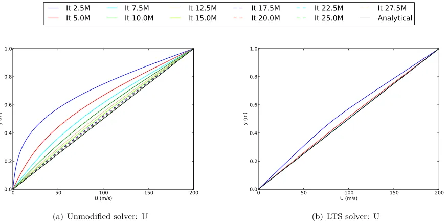
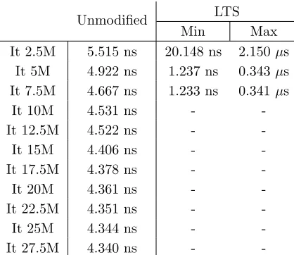
Figures7and8show the progress of the solution with respect to the number of iterations. Similar results were found for pressure andy-velocity. It is evident that the LTS solver converges to the analytical solution using much fewer iterations than the unmodified solver. Table1shows the individual cell time-step. Whereas the time-step for the unmodified solver is the same for all cells, for the LTS solver the minimum time-step is two orders of magnitude smaller than the maximum time-step. This difference allows the bigger cells, which have larger time-steps, to reach a steady state solution faster, accelerating the global convergence of the LTS solution.
200 250 300 350 400 T (K) 0.0 0.2 0.4 0.6 0.8 1.0 y (m)
It 2.5M
It 5.0M
It 7.5M
It 10.0M
It 12.5M
It 15.0M
It 17.5M
It 20.0M
It 22.5M
It 25.0M
It 27.5M
Analytical
200 250 300 350 400 T (K) 0.0 0.2 0.4 0.6 0.8 1.0 y (m)
(a) Unmodified solver: T
200 250 300 350 400 T (K) 0.0 0.2 0.4 0.6 0.8 1.0 y (m)
(b) LTS solver: T
Figure 7. Results from the unmodified and the LTS solvers for temperature
200 250 300 350 400
T (K) 0.0 0.2 0.4 0.6 0.8 1.0 y (m)
It 2.5M
It 5.0M
It 7.5M
It 10.0M
It 12.5M
It 15.0M
It 17.5M
It 20.0M
It 22.5M
It 25.0M
It 27.5M
Analytical
0 50 100 150 200
U (m/s) 0.0 0.2 0.4 0.6 0.8 1.0 y (m)
(a) Unmodified solver: U
0 50 100 150 200
U (m/s) 0.0 0.2 0.4 0.6 0.8 1.0 y (m)
(b) LTS solver: U
[image:10.612.90.523.103.318.2] [image:10.612.88.525.440.659.2]Unmodified LTS
Min Max
It 2.5M 5.515 ns 20.148 ns 2.150µs
It 5M 4.922 ns 1.237 ns 0.343µs
It 7.5M 4.667 ns 1.233 ns 0.341µs
It 10M 4.531 ns -
-It 12.5M 4.522 ns -
-It 15M 4.406 ns -
-It 17.5M 4.378 ns -
-It 20M 4.361 ns -
-It 22.5M 4.351 ns -
-It 25M 4.344 ns -
-It 27.5M 4.340 ns -
-Table 1. Simulation time-step in each iteration level, for the unmodified and LTS solvers
Unmodified LTS
It 2.5M 7h 26min 50s 9h 21min 17s
It 5M 14h 55min 57s 18h 52min 40s
It 7.5M 22h 37min 11s 28h 0min 44s
It 10M 29h 23min 21s
-It 12.5M 35h 5min 21s
-It 15M 41h 13min 13s
-It 17.5M 47h 12min 38s
-It 20M 52h 58min 3s
-It 22.5M 59h 21min 11s
-It 25M 65h 30min 11s
-It 27.5M 71h 41min 41s
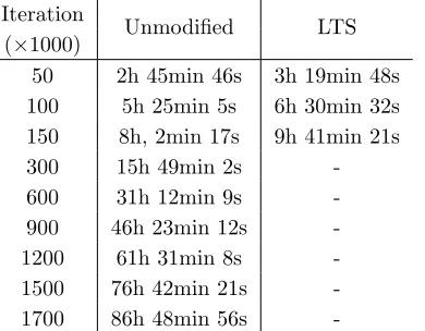
[image:11.612.201.410.119.300.2] [image:11.612.211.402.460.633.2]III.A.2. Supersonic flat plate
The following data show the flow properties along the vertical line located one reference length (0.01m) behind the leading edge of the flat plate.
The simulation has been considered converged when the difference between two solutions 5×10⁴iterations
apart was smaller than 0.01% of the upstream values. The unmodified solver reached 1.7×10⁶ iterations
before this condition was fulfilled, whereas for the LTS solver only 1.5×10⁵ iterations were required. The
computational times required to reach this convergence criterion were 86 h 48 min 56 s for the unmodified solver and 9 h 41 min 21 s for LTS solver, thus achieving convergence 8.96 faster than the unmodified solver.
Figures 9 to 11 show the progress of the solution with the number of iterations. Similar results were found for temperature. In Figure11thex-velocity is also compared with the velocity profile from Ref. 18.
Iteration
Unmodified LTS
(×1000)
50 2h 45min 46s 3h 19min 48s
100 5h 25min 5s 6h 30min 32s
150 8h, 2min 17s 9h 41min 21s
300 15h 49min 2s
-600 31h 12min 9s
-900 46h 23min 12s
-1200 61h 31min 8s
-1500 76h 42min 21s
-1700 86h 48min 56s
-Table 3. Computational time required to reach each iteration level, for the unmodified and LTS solvers
0.0 0.2 0.4 0.6 0.8 1.0 1.2 0.0 0.2 0.4 0.6 0.8 1.0 1.2 It 300k
It 600k It 900kIt 1200k It 1500kIt 1700k
0.0 0.2 0.4 0.6 0.8 1.0 1.2 0.0 0.2 0.4 0.6 0.8 1.0 1.2
It 50k It 100k It 150k
1.20 1.25 1.30 1.35 p/p∞ 0.0 0.2 0.4 0.6 0.8 1.0 y/ h
(a) Unmodified solver: p
1.20 1.25 1.30 1.35 p/p∞ 0.0 0.2 0.4 0.6 0.8 1.0 y/ h
(b) LTS solver: p
[image:12.612.214.409.223.375.2] [image:12.612.87.519.414.617.2]0.0 0.2 0.4 0.6 0.8 1.0 1.2 0.0 0.2 0.4 0.6 0.8 1.0 1.2 It 300k
It 600k It 900kIt 1200k It 1500kIt 1700k
0.0 0.2 0.4 0.6 0.8 1.0 1.2 0.0 0.2 0.4 0.6 0.8 1.0 1.2
It 50k It 100k It 150k
0.00 0.02 0.04 0.06 0.08 0.10 v/U∞ 0.0 0.2 0.4 0.6 0.8 1.0 y/ h
(a) Unmodified solver: v
0.00 0.02 0.04 0.06 0.08 0.10 v/U∞ 0.0 0.2 0.4 0.6 0.8 1.0 y/ h
(b) LTS solver: v
Figure 10. Results from the unmodified and the LTS solvers fory-velocity
0.0 0.2 0.4 0.6 0.8 1.0 1.2 0.0 0.2 0.4 0.6 0.8 1.0 1.2 It 300k
It 600k It 900kIt 1200k It 1500kIt 1700k
0.0 0.2 0.4 0.6 0.8 1.0 1.2 0.0 0.2 0.4 0.6 0.8 1.0 1.2
It 50k It 100k It 150k
[image:13.612.81.528.99.300.2] [image:13.612.76.539.412.655.2]III.B. AMR
III.B.1. Supersonic wedge
Figure 12 shows Mach number contour plots for the initial and refined meshes, as well as the meshes themselves. The shock wave is resolved with higher accuracy as the cell resolution is increased. This increase in accuracy can be also observed in Figure13, where the analytical shock wave (black line) is superimposed on the previous Mach contour plots.
In Figure14, the results for pressure, temperature, and Mach number on the top boundary are compared with the analytical solution, showing again the importance of cell refinement in the proximities of the shock wave.
(a) Base mesh (b) First Refinement
(c) Second Refinement (d) Third Refinement
Figure 12. Mach number contour plots for different refinement levels
(a) Base mesh (b) First Refinement
(c) Second Refinement (d) Third Refinement
[image:14.612.89.541.192.419.2] [image:14.612.85.542.453.688.2]0.2
0.0
0.2
0.4
0.6
0.8
1.0
1.2
x/x
shock2
4
6
8
10
12
p/
p
∞Base mesh
1
strefinement
2
ndrefinement
3
rdrefinement
Analytical
0.2 0.0 0.2 0.4 0.6 0.8 1.0 1.2 x/xshock
2 4 6 8 10 12
p/
p∞
(a) Pressure
0.2 0.0 0.2 0.4 0.6 0.8 1.0 1.2 x/xshock
0.5 1.0 1.5 2.0 2.5 3.0 3.5
T/
T∞
(b) Temperature
0.2 0.0 0.2 0.4 0.6 0.8 1.0 1.2 x/xshock
2.0 2.5 3.0 3.5 4.0 4.5 5.0 5.5
M
(c) Mach number
III.B.2. Sod shock tube
Figure 15shows density contour plots for both refinement criteria, as well as the meshes themselves, for t=0.1s and t=0.2s. The two refinement criteria were ∇pp and ∇ρρ. Both the shock wave and the rarefaction
wave are resolved with high accuracy, as the cell resolution is increased. However, it is evident that the ∇pp criterion does not provide enough resolution to accurately capture the contact discontinuity. These features can also be observed in Figure 16, where the analytical solution for the shock tube is compared with the computational results.
The explanation for this lack of refinement near the contact discontinuity is that whereas density changes through this type of discontinuity, pressure does not. This makes the contact discontinuity invisible to the
∇p
p criterion, and reflects the importance of selecting an appropriate refinement criterion.
(a)∇p/pcriterion, t=0.1s
(b)∇ρ/ρcriterion, t=0.1s
(c)∇p/pcriterion, t=0.2s
[image:16.612.70.543.206.561.2](d)∇ρ/ρcriterion, t=0.2s
0.4
0.2
0.0
0.2
0.4
x/L
0.0
0.2
0.4
0.6
0.8
1.0
p/
p
L
Base mesh
AMR (
∇
p/p
)
AMR (
∇
ρ/ρ
)
Analytical
0.4 0.2 0.0 0.2 0.4 x/L 0.0 0.2 0.4 0.6 0.8 1.0 p/ pL
(a) Pressure, t=0.1s
0.4 0.2 0.0 0.2 0.4 x/L 0.0 0.2 0.4 0.6 0.8 1.0 p/ pL
(b) Pressure, t=0.2s
0.4 0.2 0.0 0.2 0.4 x/L 0.0 0.2 0.4 0.6 0.8 1.0 ρ/ ρL
(c) Density, t=0.1s
0.4 0.2 0.0 0.2 0.4 x/L 0.0 0.2 0.4 0.6 0.8 1.0 ρ/ ρL
(d) Density, t=0.2s
[image:17.612.82.533.58.694.2]IV.
Conclusions
The local time stepping (LTS) and adaptive mesh refinement (AMR) techniques have been implemented into one of the OpenFOAM compressible flow solvers, rhoCentralFoam. The implementation of the LTS technique has resulted in a significant reduction of the computational time for the simulation of the Couette flow, matching the analytical solution to within 1.03% error 2.56 times faster than the unmodified solver. A more significant improvement was obtained for the flat plate, as the solution converged 8.96 times faster using local time stepping. The AMR technique has also been successfully implemented in rhoCentralFoam, pro-ducing an improved solution using significantly fewer computational cells compared with meshing procedures using global refinement. Future studies will apply the AMR and LTS techniques to additional high-speed compressible flow situations in order to fully categorise the extent of the computational time saving when applying these features.
References
1Maciel, E. and Pimenta, A., “Reentry Flows in Chemical Non-Equilibrium in Three-Dimensions,”WSEAS Transactions on Mathematics, Vol. 11, No. 3, March 2012, pp. 262–282.
2Georgiadis, N., Yoder, D., Vyas, M., and Engblom, W., “Status of Turbulence Modeling for Hypersonic Propulsion
Flowpaths,”Theoretical and Computational Fluid Dynamics, Vol. 28, No. 3, June 2014, pp. 295–318.
3Bonfiglioli, A. and Paciorri, R., “Hypersonic Flow Computations on Unstructured Grids: Capturing vs.
Shock-Fitting Approach,”40th Fluid Dynamics Conference and Exhibit, June 2010.
4Fico, V., Emerson, D., and Reese, J., “A Parallel Compact-TVD Method for Compressible Fluid Dynamics Employing
Shared and Distributed-Memory Paradigms,”Computers & Fluids, Vol. 45, 2011, pp. 172–176.
5Wang, C., Wu, S. P., and Cao, N., “Application of Improved TVD Scheme in Hypersonic Heat-Flux Simulation,”Advanced Materials Research, Vol. 588, 2012, pp. 1822–1826.
6Gnoffo, P. and White, J., “Computational Aerothermodynamic Simulation Issues on Unstructured Grids,”37th AIAA Thermophysics Conference, June 2004.
7Gnoffo, P. A., “Simulation of Stagnation Region Heating in Hypersonic Flow on TetrahedralGrids,”18th AIAA CFD Conference, June 2007.
8Saunders, D. A., Yoon, S., and Michael, J. W., “An Approach to Shock Envelope Grid Tailoring and Its Effect on Reentry
Vehicle Solutions,”45th AIAA Aerospace Sciences Meeting and Exhibit, Jan. 2007.
9Sha, P., Dinghua, P., Guohao, D., Zhengyu, T., Yueming, Y., and L., H., “Grid Dependency and Convergence of
Hypersonic Aerothermal Simulation,”Acta Aeronautica et Astronautica Sinica, Vol. 31, No. 3, March 2010.
10Gnoffo, P., “An Upwind-Biased, Point-Implicit Relaxation Algorithm for Viscous, Compressible Perfect-Gas Flows,”
Tech. rep., NASA Technical Report 2953, 1990.
11Wright, M., Candler, G., and Bose, D., “Data-Parallel Line Relaxation Method of the Navier-Stokes Equations,”AIAA Journal, Vol. 36, No. 9, Sept. 1998.
12www.openfoam.com, Accessed: 2014-10-23.
13Greenshields, C., Weller, H., Gasparini, L., and Reese, J., “Implementation of Semi-Discrete, Non-Staggered Central
Schemes in a Colocated, Polyhedral, Finite Volume Framework, for High-Speed Viscous Flows,”Journal for Numerical Methods in Fluids, Vol. 63, 2010, pp. 1–21.
14Guti´errez, L. F., Tamagno, J. P., and Elaskar, S. A., “High Speed Flow Simulation Using OpenFOAM,” Mec´anica Computacional, Vol. XXXI, 2012, pp. 2939–2959.
15Kurganov, A. and Tadmor, E., “New High-Resolution Central Schemes for Nonlinear Conservation Laws and
Convection-Diffusion Equations,”Journal of Computational Physics, Vol. 160, No. 1, 2000, pp. 241–282.
16Kurganov, A., Noelle, S., and Petrova, G., “Semi-Discrete Central-Upwind Schemes for Hyperbolic Conservation Laws
and Hamilton-Jacobi Equations,”SIAM J. Sci. Comput., Vol. 23, 2000, pp. 707–740.
17www.cfd-online.com, Accessed: 2014-07-15.
18Berman, H. A., Anderson, Jr., J. D., and Drummond, J. P., “Supersonic Flow over a Rearward Facing Step with
Transverse Nonreacting Hydrogen Injection,”AIAA Journal, Vol. 21, No. 12, 1983, pp. 1707–1713.