Automated Graduation using Bayesian Trans-dimensional Models

      

City, University of London Institutional Repository

Citation

:

Verrall, R. J. and Haberman, S. (2011). Automated Graduation using Bayesian Trans-dimensional Models. Annals of Actuarial Science, 5(2), pp. 231-251. doi:

10.1017/S1748499511000248

This is the unspecified version of the paper.

This version of the publication may differ from the final published

version.

Permanent repository link:

http://openaccess.city.ac.uk/3806/

Link to published version

:

http://dx.doi.org/10.1017/S1748499511000248

Copyright and reuse:

City Research Online aims to make research

outputs of City, University of London available to a wider audience.

Copyright and Moral Rights remain with the author(s) and/or copyright

holders. URLs from City Research Online may be freely distributed and

linked to.

City Research Online: http://openaccess.city.ac.uk/ [email protected]

Automated Graduation using Bayesian

Trans-dimensional Models

R.J. Verrall and S. Haberman

Cass Business School

City University London

Abstract

This paper presents a new method of graduation which uses parametric formulae together with Bayesian reversible jump Markov chain Monte Carlo methods. The aim is to

provide a method which can be applied to a wide range of data, and which does not require a lot of adjustment or modification. The method also does not require one

particular parametric formula to be selected: instead, the graduated values are a weighted average of the values from a range of formulae. In this way, the new method can be seen as an automatic graduation method which we believe that in many cases can be applied without any adjustments and provide satisfactory graduated values.

Keywords

1. Introduction

Many methods have been proposed for graduating mortality data in order to provide smoother values which can be used in practice. Parametric models, using maximum likelihood or weighted least squares estimation, are very useful when there is sufficient data. Forfar, McCutcheon and Wilkie (1988) provides a comprehensive introduction to the use of parametric models for graduation, with a particular emphasis on standard tables. Forfar et al. defined a family of models which are sufficiently broad to be able to provide satisfactory results in many cases, which they called “Gompertz-Makeham formulae”. When classical estimation methods are used for Gompertz-Makeham (GM) formula, it is necessary to fit a wide range of formula and search through these to find one particular curve which provides a satisfactory graduation. The idea of this paper is to use GM formulae, but to replace the classical estimation with a Bayesian method which does not require the process of searching through a range of candidate models to identify the best one to use. Instead, the Bayesian method calculates the posterior probability for each model and produces graduated values based on these. In effect, the graduated values are a weighted average of the values from each GM formula, where the weights are the posterior probabilities for each GM formula. If there is one GM formula which is clearly the “best” model to use, then the posterior probability should be close to 1, and the graduated values will be close to those from that formula. While this can happen in certain circumstances, it is more likely that there is some doubt about which model is the best one (as can be seen from some of the examples in Forfar et al.). In this case, the new method in this paper has some advantages since it does not require a single formula to be chosen. Instead, the graduated values are a weighted average of the values from the whole range of GM formulae using the posterior probabilities as the weights. In this way, we believe that this new method may have a further advantage over the classical

estimation methods, since it is more flexible as well as automatic. It is more flexible since it can use a combination of GM formulae, and we believe that this flexibility means that it is possible that the method could be applied to a wider range of data than the

straightforward GM formulae. However, it is unlikely that the method will prove to be appropriate for all situations: for example, it would not be appropriate for application to population data over the complete life span since there are some features such as the accident hump and infant mortality rates which cannot be modelled by any GM formula. Thus, we believe that the method will work whenever GM formulae can be used, and it is also possible that the Bayesian estimation method will extend the range of circumstances when they can be applied.

In this paper, use reversible jump Markov chain Monte Carlo methods, which are an extension of the MCMC methodology applied to graduation in the actuarial literature. The reversible jump algorithms allow us to consider cases where the dimension of the parameter vector is unknown: it is not known, a priori, how many parameters are appropriate for a particular regression. We use the generic reversible jump implementation in the package winBUGS (Lunn et al., 2000).

Bayesian methods have been transformed by the use of Markov chain Monte Carlo (MCMC) methods: see, for example Gilks et al. (1996). For example, these methods have enabled statisticians to apply complex Bayesian models to a very wide range of

applications. For specific examples, Congdon (2006) is a wide-ranging book. As mentioned above, Skollnik (2001) provides an excellent introduction with actuarial examples, and we would also recommend Johansen et al.(2010) for details of the algorithms themselves. An important extension is the use of reversible jump MCMC (RJMCMC) methods (Green, 1995), which allow the analysis of trans-dimensional models. The key idea of this is to extend the range of models so that the number of variables is also unknown. In the context of parametric models for graduation, we can therefore apply a set of models and allow the Bayesian estimation process to indicate (through the posterior distributions) which are the most appropriate for the data. This is all part of the model, and it is not necessary to make subjective decisions about how many parameters to use for the graduation. In fact, the model can be used so that the graduated values are weighted averages of values from a number of different GM models, with the weights chosen according to the posterior probability for each model. In this way, it is possible to add some flexibility to the family of GM models, which may enable them to be used when conventional estimation fails: in other words, when the parametric models are abandoned in favour of a non-parametric approach (for example). The

approach we use is implemented within winBUGS, using the RJMCMC procedures outlined in Lunn et al. (2009).

Alternative approaches that can be used when parametric modeling is not suitable include non-parametric graduation such as Whittaker graduation (Whittaker, 1923) (for which Verrall, 1993, proposed a Bayesian model, building on Taylor, 1990). These methods have the advantage that they can be more flexible and adapt better to local features of the data. However, they also suffer from some disadvantages and it cannot be claimed that they provide a universal panacea for all graduation problems. In many ways, we believe that the use of the trans-dimensional approach in conjunction with parametric models provides an ideal combination of the straightforwardness of a mathematical formula together with the flexibility which is often required in practice.

The paper is set out as follows. In Section 2, the notation and methodology of the graduation methods are outlined. Section 3 contains an introduction to the Bayesian methods we use, and Section 4 describes how these can be applied to graduation. Section 5 contains two examples of the application of the new approach to CMI data in Forfar et al. (1988), and Section 6 contains the conclusions.

2. Parametric graduation and Gompertz-Makeham models

In this section, the notation used is defined and the general class of parametric models is set out. These models were first defined by Forfar et al. (1988). We assume that data are available for a set of (not necessarily consecutive) ages. We denote the age by x, and the set of ages for which data are available by RI , where I denotes all the observed data

which are available. For the sake of notational simplicity, we assume that the age is defined as age nearest birthday, although all the methods are trivially adapted to other definitions. Then it is assumed that the observed data, I, consist of the number of deaths,

x

d , and the central exposure, E_xC, for x∈R_I. These data are to be used to estimate the force of mortality, µ_x, over a range of ages which may be larger than R_I (for example, estimated values will be produced at any missing ages, and also may be required outside the range of R_I). In this paper, we will assume that data are generated by a set of

independent lives, and will therefore exclude the possibility of duplicate policies, or the graduation of data based on amounts of insurance or annuity. The likelihood can

therefore be written as

C

x x x

I

d E

I x

x R

L

µ

e

− µ

∈

∝

∏

(see, for example, Macdonald, 1996), which is equivalent to the use of a Poisson likelihood function. The force of mortality can be estimated by maximum likelihood estimation, with a parametric model for µx inserted when carrying parametric

graduation. Many parametric models have been suggested for µx, of which two of the

x x A Bc

µ = + . While these models are usually too simple to provide satisfactory graduations, they do capture some essential properties of the progression of mortality rates over much of the range of life. The Gompertz formula models the aging effect, which is the dominant effect over (approximately) ages 50 to 90. This is so fundamental to the modelling of mortality rates that it is usually used as the base model in some sense, even when non-parametric models are employed. The Makeham model contains this aging effect, but includes a constant, A, which measures a non-age-dependent background mortality rate which is particularly important below the age of 50. Various extensions to these two models have been suggested and used, for example by the Continuous

Mortality Investigation Bureau in the UK in the construction of mortality tables for use in the insurance industry. As a part of this process, Forfar et al. (1988) suggested a general modelling framework which encompasses the Gompertz and Makeham models, but allows a much wider range of models to be fitted. Forfar et al. noticed that many of the parametric models which had been suggested for mortality could be expressed in a unified way and extended to a wider range of possible models. The advantage of this is that it provides a range of models which can be searched through in order to find a

reasonable graduation. The general model is called a Gompertz-Makeham (GM) formula, because it starts from these basic mortality models. The GM formula, of order (r,s) is

( )

, 1 1

1 1

exp

r r s

r s i i r

i i

i i r

GM x α x α x

+

− − −

= = +

 

= + _{ }

 

∑

∑

(2.1)

with the convention that the sums disappear when r=0 or s=0. With this notation, the Gompertz model is a GM(0,2) and the Makeham model is a GM(1,2). The general strategy is to investigate a large range of values of r and s in the GM formula in order to find a reasonable graduation. In order to assess whether a graduation is “reasonable”, some criteria are needed. There are a number of tests of the fit and smoothness of a graduation, but the initial sifting through possible models can be carried out using likelihood ratio test. Twice the change in the log-likelihood has (approximately) a χ_ν2 distribution, where the degrees of freedom, ν , are the change in the number of

parameters (usually 1). The usual approach is to start with a simple model (the Gompertz model) and add parameters one at a time, examining the likelihood ratio test statistic to see whether it is justifiable to add that parameter. Forfar et al. (1988) contains a number of detailed examples of this approach which are very useful in illustrating the overall approach. Each of these examples relates to one of the CMI investigations for the period 1979 to 1982, and we use the data from Section 15 (widows of life office pensioners) and Section 16 (male life office pensioners) of Forfar et al. (1988) in the examples in Section 5 of this paper.

Before setting out the alternative Bayesian estimation method, it is necessary to consider some detailed computational aspects of the GM models. It can be seen that the GM formula, (2.1), contains powers of x, which may become very large: for example,

4

to ensure that it stays in the range

[

−1,1

]

, and this can be achieved by using x u

v

−

instead

of x, where min max

2

x x

u= + , max min

2

x x

v= − and xmin and xmax are the minimum and

maximum values, respectively, of x∈R_I. Finally, the GM formulae are defined in terms

of Chebycheff polynomials of the first kind,Cn

( )

x , rather than

{

}

2 3

1, ,x x x, , , where

( )

0 1

C x = , C x₁

( )

=x and C_n+1

( )

x =2xC_n

( )

x −C_n−1

( )

x for n≥1. The reason for using these Chebycheff polynomials is again for computational efficiency, since they form an orthonormal basis: for further details of this, see Forfar et al. (1988). Thus, the exact form of the GM formula which we use is

( )

,

1 1

1 1

exp

r r s

r s

i i i i r

i i r

x u x u

GM x C C

v v

α ₋ + α _{− −}

= = +

−  − 

   

= _{ }+ _{  }

    

∑

∑

(2.2)

For the rest of this paper, GMr s,

( )

x refers to the form in (2.2) rather than (2.1). This parametric formula forms the basis for all the models we use, and the form of the model depends on which of the parameters, α_i are non-zero. One difference between the approach of Forfar et al (1988) and the approach taken in this paper is that we do not insist that the models are nested, since we are not using likelihood ratio tests to search through models. This means that we include models where α_i may be 0 for some i<r,

even though α_r is non-zero.

The specification of the model is completed by distributional assumptions, which, as stated above, are equivalent to the assumption that

~

x

d independent Poisson with mean C x x E µ

where µ_x =GMr s,

( )

x .

The Bayesian approach uses models in the form of (2.2), assumes that they are all equally likely (a priori) and estimates the posterior probability for each of them given the data. This entails assessing a total of 2r s+

models, of varying dimension and calculating the posterior probability for each of these. This is done using MCMC methods, and since the number of parameters is not the same for each model, it also entails using reversible jump methods, as described in Section 3.

3. Trans-dimensional models and Markov chain Monte Carlo methods

with many more technical details than is appropriate here. The application of the methods uses the software winBUGS, and the web page for the BUGS project contains links to many on-line resources (http://www.mrcbsu.cam.ac.uk/bugs).

At the basis of the Bayesian modeling is Bayes’ theorem, where all parameters are

assumed to be unknown random variables. Thus, the distribution of the observed data, I , is denoted by f I

(

| ,θ M

)

and depends on the unknown parameters θ for a specific model M. It is assumed that M belongs to a class of models, S_M. The model and model parameters are assigned prior distributions, f M

( )

and f

(

θ |M

)

, and the posterior distribution is given by f

(

θ,M I|

)

∝ f I

(

| ,θ M f

) (

θ|M f M

) ( )

. It can be seen from this that parameter uncertainty is included through the prior distribution of the parameters (conditional on the model); and also model uncertainty is included through the prior distribution for M. It is the inclusion of the prior distribution for M which is the new feature of this paper, and it is this which requires the use of the methods set out in Section 3.1. Note that it is assumed that a GM formula is appropriate for the data, although the values of r and s are not known. Thus, the model uncertainty included in this paper is within the family of GM models.

For graduation purposes, we require the posterior distribution of the mortality rates, µx,

given the data I. A more limited aim would be to choose a model first, and then derive the posterior distribution of µ_x, conditional on the model M and the data I:

(

_x| ,

)

(

_x| ,

) (

| ,

)

f µ M I =

∫

f µ M θ f θ M I dθ . (3.1)

Note that this is a standard Bayesian analysis, which can be used to estimate the

parameters for a particular model. The more complete problem is not to condition on M, which then enables us to include inference about the models in S_M. This is addressed in Section 3.1, and this will give the posterior probability of each model M, given the data,

I. In this way, model uncertainty (within S_M) is summarised in these posterior

probabilities. It is possible to take into account this model uncertainty when producing graduated mortality rates in two ways. Either we can choose the most likely model (a posteriori), M_max, and base the graduation on this, or we can estimate µ_x using a weighted average of all models, using the posterior probabilities for each model as the weight. In other words, the choice is between

(

x| max,

)

f µ M I (3.2)

and

(

| ,

) (

|

)

M

x M S

f µ M I P M I

∈

∑

. (3.3)

one model does indeed dominate, and we could then use (3.2). However, it is also the case that this model will then dominate the sum in (3.3) and hence the graduated mortality rates. If it is desired that the graduated rates should follow precisely a parametric curve, then (3.2) should be used, and it will be necessary to go through a similar of model choice as for classical estimation methods (as in Forfar et al., 1988). However, we believe that the added flexibility of leaving all models in the estimation, albeit with possibly very small posterior probabilities in (3.3) is very useful in the context of graduation. Also, it is often the case that there are a number of models whose posterior probabilities are quite similar and it may be difficult to decide which model is the best one to use when using (3.2). This is certainly true in Forfar et al. (1988), much of which is devoted to deciding which single model should be used to produce the graduated values. For example, Section 16.2 considers the “Choice of Order of Formula” for the male life offices pensioners data. A total of 15 models are considered, of which the

( )

1,3

GM x and 1,5

( )

GM x are identified as the best candidates, based on a battery of tests and consideration of the shape and smoothness of the graduated values. We replace this process with the Bayesian fitting procedure described in the following section.

3.1 Reversible Jump MCMC

In this section, we extend (3.1) so that the model uncertainty is also included. This, the posterior distribution of µ_x|I, taking into account model uncertainty as well as

parameter uncertainty, can be written as

(

_x|

)

(

_x| ,

) (

, |

) (

,

)

f µ I =

∫

f µ M θ f θ M I d M θ

and in some cases this distribution may be obtained in exact terms, straightforwardly. However, in most cases it is not possible to obtain the posterior distribution in closed form, for example when the model is unknown and the parameter vector is high

dimensional, or complex. In these cases, simulation methods can be highly effective and the recent advances in Bayesian methodology use simulation based on Markov chains: the so-called Markov chain Monte Carlo methods. In MCMC methods, a Markov chain

( ) ( )

(

)

{

b , b

}

₁

b

M θ

∞

= is generated whose equilibrium distribution is the required posterior

distribution, f

(

θ,M I|

)

. The distribution for any required quantity can then be approximated by a Monte Carlo average. In this case, an estimate of the mortality rate can be obtained as

(

)

(

( ) ( )

)

1

1

| | ,

N

B ta B ta

x x

a

f I f M

N

µ µ + θ +

=

≈

∑

(3.4)

(Geman and Geman, 1984, and Gelfand and Smith, 1990) and the Metropolis-Hastings algorithm (Metropolis et al., 1953 and Hastings, 1970). For more details of these

algorithms, see Johansen et al. (2010). The basic idea of MCMC methods is to simulate a sequence of values in such a way that they converge to the required posterior distribution. This is then extended to allow jumps between different models by the use of reversible jump MCMC methods. The term “reversible jump” refers to a technical property of the sampling procedure that ensures that it converges to the required posterior distribution.

Given the current state,

(

M( )b ,θ( )b

)

, a subsequent state

(

M,θ

)

is drawn from some proposal distribution π and is either accepted or rejected, so that the next state is

( ) ( )

(

1 1

)

,

b b

M + θ + , where

( ) ( )

(

1 1

)

(

(

( ) ( )

)

)

, ,

, b b

b b M M

M

θ θ

θ

+ + 

=  

(

)

(

)

if , is accepted

if , is rejected

M M

θ θ

For variable dimension models, the sampling procedure has to be designed quite carefully to ensure convergence. This involves an extension to the Metropolis-Hastings algorithm, which leads to a sampling procedure known as the reversible jump algorithm, and which was proposed by Green (1995).

3.2 Trans-dimensional models in BUGS

Bayesian models which allow for model uncertainty where the number of parameters is one of the unknown quantities are often referred to as “trans-dimensional” models. It is possible to construct computer programmes separately from first principles for each application, but winBUGS is freely available and has been designed to be “flexible software for the Bayesian analysis of complex statistical models using Markov chain Monte Carlo (MCMC) methods”. Hence, the applications in this paper make use of winBUGS, together with the RJMCMC add-ons which are also available from the BUGS project web site. There is also a useful User Manual available (“winBUGS Jump

Interface: User Manual”). This allows us to apply the type of models described above, in which the structure of the model itself is unknown. There are two main classes of models that can be used within winBUGS, one of which will be used in this paper (see Lunn et al., 2009 for more details). This is described in this section, in general terms, with the application to graduation specified in Section 4. Lunn et al. (2009) define the trans-dimensional model in terms of an unknown number of “entities of interest”, which, in graduation, will be parameters in the GM formula (ie α_i in 2.2). The number of “entities of interest” (parameters) is denoted by k, and the prior distribution for k is specified so that all values of k are equally likely (a priori) up to a maximum value of Q. This means that each parameter is either included or excluded, so that binomial distribution is the

appropriate prior for k, with parameters Q and 1

not be included in the model. Note that for a GMr s,

( )

x formula, as given by equation

(2.2), we will use two of these models: one for 1

1 r i i i x α − =

∑

and the other for

1 1 exp r s i r i i r x α + − − = +    



∑

. In the first, the parameters η η1, 2,,ηk+1 will refer to α α1, 2,,αr,

and in the second, they will refer to α α_r+1, _r+2,,α_{r s+} . Hence, we use the general notation at the moment, and define the parameter vector ψ which can be used in the model for the mean of the data:

1 1 1 1 1 1 1 2 1 2 2 1 1 1 1 1 k k k

l l k

z z z z z z θ θ θ θ θ θ ψ η ψ η ψ

ψ η ₊

                  = _{=  }         _{ }    _{ }          

. (3.5)

θ represents the current configuration of the model: in other words , θ changes as particular parameters are included or excluded from the model. This, it can be seen that it is of dimension k to match the number of parameters currently included in the model. The design matrix can be chosen to match the models which are to be fitted. For the models which we use (the GM models), each zij will be 0 or 1, and further details of this are

given in Section 4. In this way, it will be seen that the distributions of the parameters in the GM model, α_i, can be obtained from the sampled values of ψ .

Since there are two choices to make when fitting a GM model, we will use more than one of these trans-dimensional models in the application to graduation. Thus, the two terms in

(2.2), ₁

1 r i i i x u C v α ₋ = −      

∑

and ₁

1

exp

r s i i r i r x u C v α + − − = +   −     _{ }



∑

 are treated separately. These will then be combined in the mean, as specified in equation (2.1), and in this way the

RJMCMC methods will allow us to consider graduations where the number of parameters in each of these terms is unknown. This is explained in more detail in Section 4, and in this section, we consider just a single trans-dimensional model of the form of (3.5).

The distinctive aspect of (3.5) is that the value of k can be varied within the model, so that parameters can be included or excluded within the sampling procedures. The posterior distribution for k is a part of the output, giving an indication of how many parameters should be included. More importantly, the output also gives information on which parameters these are. Note that it is possible that the Bayesian model will indicate that any set of parameters can be included – there is no restriction on them being

of the parameters, η η₁, ₂,,η_k+1, is set by default in winBUGS, such that they are independently normally distributed and

[ ]

1

E η =m,Var

[ ]

η₁ =τ₁

0 j

E  =_{ }η ,Var  =_{ }η_j τ_η, ( j=2, 3,,k+1).

The values of m, τ₁ and τ_η are part of the prior specification, and will usually be chosen so that the distributions are non-informative.

4. Trans-dimensional models for graduation

In this section, we specify a trans-dimensional modelling framework which we believe is suitable for many graduations. In particular, this framework should be suitable for

graduations of mortality rates over adult ages, although it may not capture all the features that may be present at young ages. Since a GM model has two components,

1 1 r i i i x u C v α ₋ = −      

∑

and ₁

1

exp

r s i i r i r x u C v α + − − = +   −     _{ }



∑

, each of these will be modelled by a separate trans-dimensional model. Before specifying these in detail, we first consider the range of GM models which should be included in the overall framework. It should be noted that, in general, a GM model is non-linear. If r=0 or s=0 then the model is linear, but this is unlikely to occur in practice. In particular, the Gompertz term will always be needed, which means that the minimum value of s that should be considered is 2. Also, the Makeham term is often needed (r=1), and may also be necessary to

consider higher values of r in order to capture the progression of mortality rates at

younger ages. The terms in ₁

1 r i i i x u C v α ₋ = −      

∑

have to be more carefully handled, since they can cause the model to produce negative values for the mortality rates. However, it is unlikely that values of r higher than 3 will be needed since the higher terms in

1 1

exp

r s i i r i r x u C v α + − − = +   −     _{ }



∑

 usually capture shape of the mortality curve satisfactorily. For these reasons, the most complicated model we include is the GM3,6

( )

x . The trans-dimensional modelling approach will allow each parameter to be included or excluded, and we believe that this provides a sufficiently flexible framework for most graduations. The trans-dimensional models will be specified in terms of the maximal model:

( )

3 9

3,6

1 1

1 4

exp

i i i i r

i i

x u x u

GM x C C

v v

α ₋ α _{− −}

= =

−  − 

   

= _{ }+ _{  }

    

∑

∑

. (4.1)

The parameter vector is

(

α α₁, ₂,,α₉

)

and, since the Gompertz term is always needed,

4

is the least complicated that can be considered, and so we also always include α₁, although its posterior distribution can have a mean of 0 if it is not really needed. This leaves 6 other parameters,

(

α α₂, ₃

)

and

(

α α α α₆, ₇, ₈, ₉

)

, which can be included or excluded, making a total of 64 different models in the trans-dimensional framework. Each of the two sets of parameters,

(

α α2, 3

)

and

(

α α α α6, 7, 8, 9

)

, will be modelled using

a separate trans-dimensional model of the format of (3.5), and we specify these below. As can be seen from (3.5), the first parameter in ψ is always included in the model, and we therefore specify models for

(

α α α1, 2, 3

)

and

(

α α α α α5, 6, 7, 8, 9

)

, leaving the prior

distribution for the remaining parameter, α₄, to be specified separately.

We define ψ(1)

and ψ(2)

as follows (1) 1 1 (1) (1) 2 2 (1) 3 3

1 0 0

1 1 0

1 0 1

ψ α

ψ ψ α

ψ α           =_{  }= _{ }     _{   }   (4.2) and (2) 5 1 (2) 6 2 (2) (2) 7 3 (2) 8 4 (2) 9 5

1 0 0 0 0

1 1 0 0 0

1 0 1 0 0

1 0 0 1 0

1 0 0 0 1 α ψ

α ψ

ψ ψ α

α ψ α ψ                     = =               _{   }   (4.3) Hence (1) 1 1

α ψ= , (1) (1)

2 2 1

α =ψ −ψ , (1) (1)

3 3 1

α ψ= −ψ

and α ψ₅ = ₁(2), α ψ_i = _i(2)₋₄ −ψ₁(2)(i=6, 7, 8, 9).

As mentioned in Section 3.2, the prior distribution for the number of parameters included is chosen such that all models are equally likely (a priori). In other words, P M

(

(1)

)

=2−2

for the first trans-dimensional component, and P M

(

(2)

)

=2−4 for the second. The prior

distributions of the optional parameters, conditional on ( )j

M ( j=1, 2), is set by default such that they are independently normally distributed. It is possible to specify the model in winBUGS such that all parameters have the same prior mean and variance, or such that the first parameter has a different mean and variance. For the first trans-dimensional model, (4.2), we give all the parameters the same mean and variance, but for the second, (4.3), we give the first parameter a different prior mean and variance in order to

way to proceed is to first fit a simple Gompertz model to the data, and use the maximum likelihood estimates of the parameters as the prior means. In summary, the prior

distributions are specified as follows (with all parameters being independent, a priori).

(

α α α1, 2, 3

)

~ independent normal with mean 0 and variance 2 1

σ

(

)

4 ~N a L1,

α , α₅ ~N a L

(

₂,

)

,

where a a₁, ₂ are the maximum likelihood estimates of the parameters in the simple Gompertz model and L is a value which is large enough that these prior distributions are non-informative (in the examples, we use L = 10,000),

(

α α α α6, 7, 8, 9

)

~ independent normal with mean 0 and variance 2 2

σ

2 2

1 , 2 ~

σ σ− −

independent Γ

(

0.001, 0.001

)

.

Finally, it is necessary to place some basic restrictions on the values of the parameters

(

α α α1, 2, 3

)

, in order to ensure that the values of the mortality rates, µx, should all be

positive. Clearly, negative values are not practically justifiable, and they may cause the programme to crash when it tries to calculate ln

( )

µ_x in the log-likelihood. Thus, we

place restrictions to ensure that

3 1 1 0 i i i x u C v α ₋ = −  _{ >}

 

 

∑

at low ages, noting that

1 1

exp

r s i i r i r x u C v α + − − = +   −     _{ }



∑

 will be close to zero at low ages. Firstly, we ensure that

1 0

α > , as a basic requirement of a sensible GM model. Secondly, we note that the

second derivative of

3 1 1 i i i x u C v α ₋ = −      

∑

should be positive, to reflect the expected shape of this contribution to the mortality rates at low ages: this is expected to be convex. Hence, the second restriction is α >3 0. Finally, the value of α2 is restricted so that

3 1 1 0 i i i x u C v α ₋ = −  _{ >}

 

 

∑

when x u 1

v

−

= − . This means that α α α₁− ₂ + ₃>0 and hence the

final restriction is α2 <α α1+ 3. In the MCMC algorithms in winBUGS, it is

straightforward to ensure that these restrictions are not violated by simply replacing the sampled value when it is not satisfactory. Thus, for example, negative values of α₁ and

3

5. Examples

We illustrate the application of the automatic graduation method using two sets of data, which are taken from Forfar et al. (1988). It should be emphasized that the same

programme is used for each data set, and the differences in the results are entirely due to the differing natures of the data themselves. It will be seen that this graduation method deals satisfactorily with the data in each case, without the need for any intervention from the graduator, and it is for this reason that we call this an “automatic” graduation method.

In all cases, we used an initial burn-in of 50,000 iterations (these are values which are discarded), and found that the models had converged. In general, we would expect that 50,000 burn-in iterations would be sufficient for convergence, but it is always

recommended that this is checked (see, for example, Johansen et al., 2010, for tools to monitor convergence). After this, we ran 50,000 iterations and used these for the results. Thus, in equation (3.4), B = 50,000, N = 50,000 and t = 1.

5.1 Example 1

The data for the first example are taken from table 15.5 of Forfar et al. (1988), and consist of data from the CMI relating to the numbers of deaths for Pensioners’ widows over the calendar years 1979-82, grouped by age nearest birthday. Forfar et al. (1988) concluded that a satisfactory graduation for µ_x could be provided by the simple

Gompertz model, GM0,2

( )

x . Note that Forfar et al. (1988) used u=70 and v=50,

whereas we use min max

62.5 2

x x

u= + = , max min

45.5 2

x x

v= − = . Hence, the parameter

estimates cannot be directly compared, although it is straightforward to make a simple conversion to obtain corresponding values. Since Forfar et al. (1988) concluded that a Gompertz model provided a satisfactory graduation, this example provides a test of whether the new graduation method is able to come to a similar conclusion: in effect, we would expect the Bayesian model to tell us that none of the optional parameters is required. As was explained in Section 4, we always start from the Makeham model, and we would therefore also expect that the posterior mean of α₁ should be close to 0. We

Parameter Estimate

1

α _0.000012466

2

α _0.000047652

3

α _0.000063398

Table 1: Estimates of the parameters in the first part of the GM formula for the data from Example 1 of Forfar et al. (1988).

It can be seen that these parameter estimates are so small will have no evident effect on the graduated values whether or not they are included in the model.

The second trans-dimensional model indicates that none of the optional parameters in

1 1

exp

r s i i r i r

x u C

v

α

+

− − = +

  − 

 

 _{ }



∑

 should be included, leaving just α4 and α5 in the model. The

conclusion from this is that the basic Gompertz model, _x exp _{4 5} x u

v

µ = _α α+ _ − __

 

  is

indeed most likely to provide a suitable graduation for these data. As noted in Section 3, we could either base inferences about the mortality rates on the most likely model or we can use a weighted average of all models, with the most likely models getting the most weight: see (3.2) and (3.3). In this paper, we use (3.3) and base the estimates of the mortality rates on the means of their posterior distributions. Table 2 shows the estimates

of the parameters in ₁

1

exp

r s i i r i r

x u C

v

α

+

− − = +

  − 

 

 _{ }



∑

.

Parameter Estimate

4

α _-4.1908

5

α _3.8792

6

α _-0.0191

7

α _-0.0194

8

α _-0.0212

9

α _-0.0293

Table 2: Estimates of the parameters in the second part of the GM formula for the data from Example 1 of Forfar et al. (1988).

model using u=62.5 and v=45.5 are –4.2005 and 3.9281, which can be compared with the estimates of α₄ and α₅ in Table 1.

age

log(

m

or

tal

it

y

r

at

e)

20 40 60 80 100

-8

-6

-4

-2

[image:17.612.96.417.147.372.2]

0

Figure 1. Crude mortality rates, together with graduated rates from Forfar et al. (solid line) and from the Bayesian model (dashed line) using the posterior weights to average over all models, for the data from Example 1.

Figure shows the results of the graduation (plotted on the log scale), together with the Gompertz curve fitted by Forfar et al. (1988). The graduated rates for the Bayesian model are obtained by averaging over the models using the posterior probabilities in (3.3), which explains why they do not follow exactly a straight line. We believe that this is the best way to proceed in general, and it can be seen that the new automatic graduation method has produced graduated values which are very close to those which were deemed to be suitable in Forfar et al.

To test the fit of the graduation, the same tests can be applied as in Forfar et al. (1988). The number of parameters is not completely determined in the Bayesian method, although it would be reasonable to assume that it is close to 2, since the only significant parameters which were indicated should be included are α4 and α5. The

2

To conclude, this example has shown that the Bayesian model has produced graduated values which are very close to those of the Gompertz model, without the need for any input or model choice.

5.2 Example 2

This example considers a case which is not as straightforward as example 1, and uses the CMI data from table 16.5 of Forfar et al. (1988). These data come from the mortality experience of male pensioners over the calendar years 1967-70, and Forfar et al. concluded, after considering a number of different possible models, that a GM(1,3) model was most suitable for graduating these data. For comparison purposes, the fitted GM(1,3) model in Forfar et al. was

2

63.5 63.5

0.00557291 exp 5.4677 6.007755 1.3219 2 1

44.5 44.5

x

x x

µ = + _− + _ − _− _ _ − _ − __

  _   _

 

.

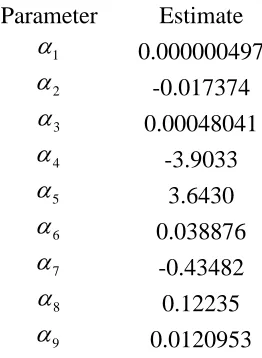
For this example, the Bayesian model suggests that a different model is more appropriate, and Table 3 shows that parameter estimates.

Parameter Estimate

1

α _0.000000497

2

α _-0.017374

3

α _0.00048041

4

α _-3.9033

5

α _3.6430

6

α _0.038876

7

α _-0.43482

8

α _0.12235

9

[image:18.612.148.279.334.513.2]

α _0.0120953

Table 3: Estimates of the parameters for the Bayesian model, for the data from Example 2 of Forfar et al. (1988).

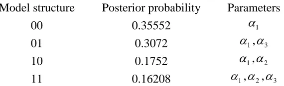
The posterior probabilities for the models in the first part of the GM formula are shown in Table 4. The 0’s and 1’s in the first column refer to whether α₂ and α₃ should be

Model structure Posterior probability Parameters

00 0.35552 α1

01 0.3072 α1,α3

10 0.1752 α1,α2

[image:19.612.163.448.85.172.2]

11 0.16208 α1,α2,α3

Table 4. Posterior probabilities for the set of possible models for the first part of the GM formula

Table 4 shows that, although the model structure 00 (with just α₁) is the most likely model (concurring with the choice of the GM(1,3) in Forfar et al. (1988), there are also reasonable posterior probabilities for the other models. Table 5 shows the marginal probabilities that each parameter should be included. When the fitted mortality rates are calculated using the weighted average of these models, the effect of these probabilities will be seen at early ages.

Parameter Marginal probability

2

α _0.33728

3

α _0.46928

Table 5. Marginal posterior probabilities for the parameters in the first part of the GM formula.

Similarly, Tables 6 and 7 show the corresponding posterior probabilities for the second part of the GM formula.

Model

structure Posterior probability Parameters

0110 0.27892 α4,α5,α7,α8

0100 0.27736 α4,α5,α7

1110 0.21612 α4,α5,α6,α7,α8

1100 0.08314 α4,α5,α6,α7

0111 0.04944 α4,α5,α7,α8,α9

1111 0.04078 α4,α5,α6,α7,α8,α9

0101 0.03856 α4,α5,α7,α9

[image:19.612.188.477.481.648.2]

1101 0.01568 α4,α5,α6,α7,α9

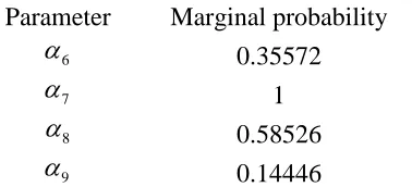
Parameter Marginal probability

6

α _0.35572

7

α ₁

8

α _0.58526

9

[image:20.612.191.380.85.171.2]

α _0.14446

Table 7. Marginal posterior probabilities for the parameters in the second part of the GM formula.

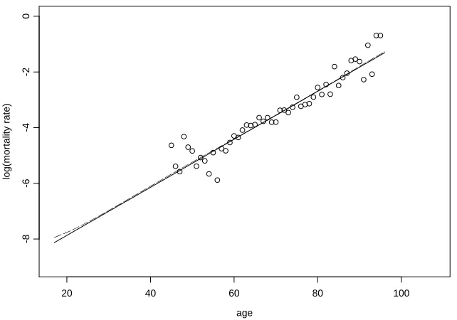
The model fitted by Forfar et al., a GM(1,3) corresponds to the model structure 1000, with just α₆ being included. It is interesting to note that the Bayesian model disagrees

with this, concluding that the parameter which definitely needs to be included is α₇ (with

age

log(

m

or

tal

it

y

r

at

e)

20 40 60 80 100

-6

-4

-2

[image:21.612.96.431.104.340.2]

0

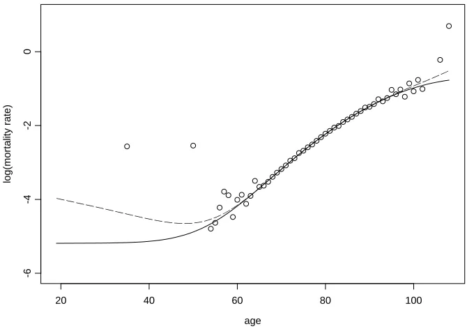
Figure 2. Crude mortality rates, together with graduated rates from Forfar et al. (solid line) and from the Bayesian model (dashed line), for the data from Example 2.

x x

xxxxxxxxxxxxxxxxxx xxxxxxx

xxxxx xxxx

xxx xxxx

x x

x x

x x

x x

x

age

mo

rta

lity

r

a

te

20 40 60 80 100

0.

0

0.

2

0.

4

0.

6

0.

8

1.

[image:22.612.104.455.104.358.2]

0

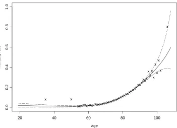
Figure 3. Crude and graduated mortality rates, together with the 95% sheaf for the results of the Bayesian model.

All of the usual tests of the graduation can be applied. For example, we can compare the results of the tests for the Bayesian graduation with those in Table 16.3 of Forfar et al.

Comparison of total actual deaths (A) and total expected (E):

Forfar et al Bayesian Model

Total A–E 1.00 –0.93

Ratio A/E 100.00 100.00

Signs Test:

Forfar et al Bayesian Model

Number of + 23 22

Number of – 24 25

P(pos) 0.5000 0.3854

Runs test:

Forfar et al Bayesian Model

Number of Runs 29 29

P(runs) 0.9304 0.9304

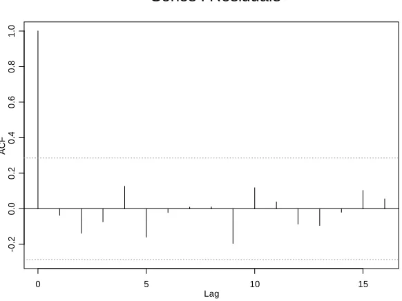
Bayesian model, together with the 95% confidence limits. It can be seen from this that none of the autocorrelations is significant.

Lag

A

CF

0 5 10 15

-0

.2

0

.0

0

.2

0

.4

0

.6

0

.8

1

.0

[image:23.612.104.395.129.347.2]

Series : Residuals

Figure 4. Autocorrelations of the residuals from the Bayesian model for the data from Example 2.

xxxxxxxxxxxxx xxxxxxxx

xxxx xxxx

xxxxx xxxx

xxxx xxxx

xxxx xxxx

xxxx xxxx

xxxx xxxx

xxxx xxxx

xxxxxx x

xx xxxx

age

log(

m

or

tal

it

y

r

at

e)

20 40 60 80 100

-6

-4

-2

[image:24.612.102.415.99.323.2]

0

Figure 7. Crude mortality rates and graduated rates for the(???) population data, from age 18 upwards.

6 Conclusions

This paper has proposed a new method for graduating mortality data, which we believe to be suitable for data over adult ages. The method has the great advantage that it is

References

Broffit, J.D. (1988). Increasing and increasing convex Bayesian graduation. Transactions of Society of Actuaries, Vol. 40, pp 115–148.

Carlin, B.P. (1992). A simple Monte Carlo approach to Bayesian graduation. Transactions of Society of Actuaries, Vol. 44, pp 55–76.

Congdon, P. (2006). Bayesian Statistical Modelling, John Wiley.

Czado, C., Delwarde, A., Denuit, M. (2005). Bayesian Poisson log-bilinear mortality projection. Insurance: Mathematics and Economics Vol. 36 (3), pp 260–284.

Forfar, D.O., McCutcheon, J.J. and Wilkie, A.D. (1988). On Graduation by Mathematical Formula. Journal of the Institute of Actuaries, Vol. 115, pp 1-149.

Gamerman, D., Migon, H.S. (1993). Bayesian dynamic hierarchical models. Journal of the Royal Statistical Society Series B, Vol. 55 (3), pp 629–642.

Gelfand, A.E. and Smith, A.F.M. (1990). Sampling-based approaches to calculating marginal densities. Journal of the American Statistical Association, Vol. 85, pp 398-409.

Gelman A., Carlin J.B., Stern H.S., and Rubin D.B. (1995). Bayesian Data Analysis. Chapman and Hall, London.

Geman, S. and Geman, D. (1984) Stochastic relaxation, Gibbs distribution, and the Bayesian restoration of images. IEEE Transactions on Pattern Analysis and Machine Intelligence, Vol. 6, pp 721-741.

Gompertz, B. (1825). On the Nature of the Function Expressive of the Law of Human Mortality, and on a New Mode of Determining the Value of Life Contingencies. In a letter to Francis Bailey. Philosophical Transactions of the Royal Society, Vol. 115, pp 513-583.

Green, P.J. (1995). Reversible jump Markov chain Monte Carlo computation and Bayesian model determination. Biometrika Vol. 82, pp 711-732.

Hastings, W.K. (1970). Monte Carlo sampling methods using Markov chains and their applications. Biometrika, Vol. 57, pp 97-109.

Heligman and Pollard (1980). The Age Pattern of Mortality. J.I.A. Vol. 107, pp 49-80.

Johansen, A.M., Evers, L. and Whiteley, N. (2010). Monte Carlo Methods. Lecture Notes, Department of Mathematics, University of Bristol.

Lunn, D.J., Best, N. and Whittaker, J.C. (2009) Generic reversible jump MCMC using graphical models. Statistics and Computing, Vol. 19, pp 395- 408.

Lunn, D.J., Thomas, A., Best, N., and Spiegelhalter, D. (2000). WinBUGS – a Bayesian modelling framework: concepts, structure, and extensibility Statistics and Computing, Vol. 10, pp 325-337.

Macdonald, A.S. (1996) An Actuarial Survey of Statistical Models for Decrement and Transition Data. I: Multiple State, Binomial and Poisson Models. British Actuarial Journal, Vol. 2, pp 129-155.

Makeham, W. (1859). On the Law of Mortality and the Construction of Annuity Tables, Journal of the Institute of Actuaries, Vol. 8, pp 301-310.

Metropolis, N., Rosenbluth, A.W., Rosenbluth, M.B., Teller, A.H. and Teller, E. (1953). Equation of state calculations by fast computing machines. The Journal of Chemical Physics, Vol. 21, pp 1087-1092.

Neves, César da Rocha, Migon, H.S. (2007) Bayesian graduation of mortality rates: An application to reserve evaluation Insurance: Mathematics and Economics Vol. 40 pp 424– 434

Scollnik, D.P.M. (2001). Actuarial Modeling with MCMC and BUGS. North American Actuarial Journal, Vol. 5 (2), pp 96-124.

Taylor, G. (1990) A Bayesian Interpretation of Whittaker-Henderson Graduation. Paper presented to the Risk Theory seminar, Mathematschers Forschungsinstitut, Oberwolfach, Federal Republic of Germany.

Verrall, R.J. (1993) A State Space Formulation of Whittaker-Henderson Graduation, with Extensions. Insurance: Mathematics and Economics, Vol. 13, pp 7-14.