A fixed effects ordered choice model with flexible thresholds with an application to life-satisfaction

City, University of London Institutional Repository

Citation

:

thresholds with an application to life-satisfaction. London: City University London.

This is the published version of the paper.

This version of the publication may differ from the final published

version.

Permanent repository link:

Link to published version

:

Copyright and reuse:

City Research Online aims to make research

outputs of City, University of London available to a wider audience.

Copyright and Moral Rights remain with the author(s) and/or copyright

holders. URLs from City Research Online may be freely distributed and

linked to.

Department of Economics

A fixed effects ordered choice model with flexible thresholds

with an application to life-satisfaction

Patricia

Cubí

‐

Mollá

City University London 

Firat

Yaman

City University London 

Department of Economics

Discussion Paper Series

No. 1

4/1

0

A …xed e¤ects ordered choice model with ‡exible thresholds with

an application to life-satisfaction

Patricia Cubí-Mollá1 F¬rat Yaman2

JEL classi…cation: C23, C25, I31

Keywords: Ordered choice, …xed e¤ects, subjective well-being, life-satisfaction

Abstract

In many contexts reported outcomes in a rating scale are modeled through the existence

of a latent variable that separates the categories through thresholds. The literature has not

been able to separate the e¤ect of a variable on the latent variable from its e¤ect on threshold

parameters. We propose a model which incorporates (1) individual …xed e¤ects on the latent

variable, (2) individual …xed e¤ects on the thresholds and (3) threshold shifts across time

de-pending on observables. Importantly, the latent variable and the threshold speci…cations can

include common variables. In order to illustrate the estimator, we apply it to a model of life

satisfaction using the GSOEP dataset. We demonstrate that important di¤erences can arise

depending on the choice of the model. Our model suggests that threshold shifts are statistically

and quantitatively important. Factors which increase reported life-satisfaction are due both

to positive e¤ects on the latent variable AND to shifting thresholds to the left, while factors

which decrease reported life satisfaction are due to negative e¤ects on the latent variable AND

to shifting thresholds to the right.

1_{Department of Economics, City University London. Email: [email protected].} 2

1

Introduction

Many variables and outcomes of interest in the social sciences are reported in rating scales. Some

of these separate the categories along pre-speci…ed thresholds, such as categorical grades in school

(A to E, 10 to 1, etc.), but many others do not. Surveyed individuals are often asked about their

opinion on a certain statement or political issue with answer categories ranging from “Strongly

agree” to “strongly disagree”, their self-assessed health or well-being on a range from 0 to 10, or

1 to 5, how much they value certain things in life, such as family, friends, work, etc. with answers

ranging from “very much” to “not at all”, or how they assess their pro…ciency in a certain skill or

task, such as language ‡uency with answers ranging from “very well” to “not at all”. These rating

scales are in wide use in disciplines as diverse as economics, psychology, and medicine (in rating

the severity of pain, for example).

The ordinal (non-cardinal) nature of these variables has given rise to models of ordered choice

such as the ordered probit and ordered logit models, and recent contributions have developed

consistent and/or e¢ cient (in the sense of using all sample observations with variation in the

de-pendent variable) estimators for the ordered logit, which are all based on a dichotomization of the

dependent variable and the application of Chamberlain’s (1980) conditional logit model

(Winkel-mann and Winkel(Winkel-mann (1998), Das and van Soest (1999), Hamermesh (2001), Ferrer-i-Carbonell

and Frijters (2004), Baetschmann et al. (2015)). All of these applications have assumed that the

thresholds that divide one category from the other are …xed over time (but not necessarily across

individuals). This is due to the fact that in ordered choice models the e¤ect of a variable on the

level of the latent variable cannot be separately identi…ed from the variable’s e¤ect on the level

of the thresholds. We suspect that researchers have been long aware of this, but the …rst explicit

exposition of this problem goes back to Terza (1985). If thresholds do change systematically with

observed variables, then the coe¢ cient estimates in the aforementioned papers are not e¤ects on the

locations (which might have changed themselves), and thus contain very little information, since

even the sign cannot be interpreted in its e¤ect on the latent variable.

We propose a model which can identify e¤ects of variables on the latent variable from e¤ects on

the thresholds. To our knowledge this is the …rst paper which does this in the absence of objective

measures of the latent variable (as done by Lindeboom and van Doorslaer (2004) for health) or of

explicit anchoring vignettes (such as Bago d’Uva et al. (2011)). We use the Amalgamated

Condi-tional Logit Regression (ACLR) proposed by Mukherjee et al. (2008)3 and extend it by including

dependent variables which re‡ect the survey individuals’answers to questions about their current

outcome, but also their answers relating to the previous survey period’s outcome. The latter is

NOT the lagged dependent variable. Rather it is the individual’s assessment today about her

out-come last year. We illustrate our model by applying it to the outout-come of life-satisfaction in the

German Socio-Economic Panel. The application suggests that threshold shifts are statistically and

quantitatively important. For example, about a third of the coe¢ cient on household income in a

model with …xed thresholds can in fact be attributed to a shift in thresholds.

Whether a change in the reported outcome is due to a change in the underlying latent variable

or due to a change in the threshold might at …rst seem like an arcane question, but the inference,

implications, and possibly political consequences can be widely di¤erent between the two cases.

Consider …rst a simple example: In the British higher education system a grade of at least 70 (out

of 100) is considered a “…rst class” grade. Conceivably, a …rst class graduation grade might be

considered a necessary condition for a popular and attractive employer to consider an applicant for

a job interview. Now suppose the proportion of “…rst class” grades increases over time. Since the

threshold is …xed, one would be inclined to infer that students seem to be getting “better”in some

sense, but that is so only if we interpret the latent variable as the actual grade (a number between

3_{Baetschmann et al. (2015) call this estimator “blow-up and cluster” (BUC) and demonstrate its strong small}

0 and 100). However, the result might be due to the university becoming more generous in its

marking, so that a particular student might receive 70 marks today, but would have received less

for the same performance a few years earlier. If we interpret the latent variable as “knowledge” or

“quality of knowledge”, then the increased proportion of …rst class grades could be a re‡ection of

either more knowledgeable students, or as a laxation of marking standards. Clearly the distinction

would be of interest to educational policy-making.

Another increasingly important …eld in which the distinction between latent variable and

thresh-old changes is crucial is the measurement and study of subjective well-being and happiness.

Mea-sures of well-being are increasingly suggested as substitute or at least complementary meaMea-sures to

GDP that should be targeted by governments (see for example HM Treasury Budget (2010), OECD

(2011) or Dolan et al. (2011)). Since these measures re‡ect the entirety of the human experience, it

is argued, they have the potential to be more complete and even accurate compared to GDP which

includes only those goods which can be priced in the market (thus excluding things like the value

of clean air, social and physical safety, biodiversity etc.). A non-market goodx could in principle

be “priced”by inferring from regression coe¢ cients the amount of income that an individual would

give up to compensate for a unit-increase in x to keep her latent variable constant.4 But what

exactly should the social welfare function be? If it is the sum of all individual reported levels of

well-being(Y =PN_i=1yi), we need not worry about the source of changing values ofy, since both

threshold and latent variable changes will be observationally equivalent. But if the social welfare

function is over the latent variable (Y = PN_i=1y_i), as it probably should be if we consider this

to be the actual emotional state of an individual, then the distinction is important. Threshold

shifts to the left (making it easier to report higher values of well-being) would increaseY, but leave

Y unchanged. We imagine a policy-maker would like to know to what extent changes in Y are

re‡ecting changes inY .

4

It is not our intention to participate in a debate about the merits of using well-being instead or along with GDP.

2

Modeling

We follow here the conventional choice of setting up the ordinal model as a latent variable model.

That is the individual i at any given point of time t has a subjective evaluation of the question

she is being asked (her health status, opinion, life-satisfaction, etc.). The question can only be

answered by picking one out of an ordered list of answers. We index the possible answer categories

byk_{2 f}1; :::K_g. The individual’s evaluation of her underlying latent variable we denotey_it. This

evaluation translates into the reported outcomeyit, such that

yit=k , k_it 1 < yit kit (1)

The latent variable is speci…ed as

y_it=Xit + i+ it (2)

where the distribution of i is left unspeci…ed and is allowed to correlate withXi, and it is i.i.d.

logistic (with location 0 and scale 1) acrossiand t.

2.1 Threshold model

If k_it= k_i, we have all the necessary building blocks to apply Chamberlain’s conditional logit model

for a pre-speci…ed dichotomization ofy, or to apply one of the estimators based on the conditional

logit model which use all possible dichotomizations (minimum distance, ACLR). This speci…cation

of the threshold parameters is quite ‡exible, but it does impose that distances between any two

thresholds are preserved over time, or

k

it = ki;t s

and that the di¤erence of the kth threshold between two individuals is constant over time:

k

it kjt = ki kj

In this paper we decompose the thresholds into an individual- and threshold-speci…c,

time-invariant component, and a component which modi…es the thresholds linearly in parameters:

k

it= ki +Zit (3)

Thus,

k

it kjt = ki kj + (Zit Zjt)

andyit > yis does not necessarily imply yit> yis. Equations 1, 2 and 3 imply

yit=k , ki 1 < Xit Zit + i+ it ki (4)

Clearly, in this equation is not separately identi…ed from for common variables inX and Z, or

in other words, the estimate of will incur a level-bias on the order of .

2.2 The remembered outcome

In most surveys the surveyed individual is asked to rate her current outcome. However, the surveyed

individual might in addition be asked about the current outcome and about her outcome at some

point in the past. In that case we need to distinguish between the survey time, which we will

be subscripting, and thereference time, which we will be superscripting. Thus, yt

it is the reported

outcome for individualisurveyed at timetand where the evaluation refers to the time at which the

individual is surveyed. In contrasty_itt 1 is the reported outcome for individualisurveyed at timet

but where the evaluation refers to theprevious time at which the individual is surveyed: it is how

the individual remembers her outcome. Assuming the individual to have an accurate recollection

of her previous outcome, and having time-invariant thresholds, a di¤erence between yt_it and y_itt 1

would be due to a change in the individual’s latent variable. Our threshold speci…cation also allows

this to be due to changes in the threshold parameters –provided that the thresholds of timet are

applied to all questions at survey time t. A prominent example would be the e¤ect of income or

is: the barrier that divides the rich from the non-rich always seems to be above one’s own wealth.

A third possibility would be that the individual does not accurately recall her previous state. We

assume that theremembered latent variable at survey timet is the non-random component of the

latent variable at reference time t 1 amended by an additive recall erroruit. Since the error in

the latent variable it is assumed to be identically and independently (of X) distributed, one can

interpret it as a merely transitory component that in‡uences the reported answer at the time of the

survey (the “mood” of the surveyed person). Thus, we assume that the individual does remember

her circumstances of the previous survey time (as re‡ected in theX), but not the purely transitory

aspect that contributed to her answer on that day. The recall erroruit can be interpreted as both

a false recollection and/or as a discrepancy between the points of time in a past time period (the

surveyed individual questioned about her outcome “last year” might not refer to the point of time

at which she was surveyed in the previous year). We write:

yt_it 1=k _, k_it 1 < y_{i;t 1} i;t 1+uit=Xi;t 1 +uit kit

This, together with equations 2 and 3 give

y_itt 1 =k _, k_i 1 < Xi;t 1 Zit + i+uit ki (5)

This is the equation which identi…es and separately, even ifX and Z share common variables,

since the variables inX enter with a one-period lag compared toZ.

We emphasize that this derives from the application of thresholds it rather than i;t 1 to ANY

question asked at survey timet. We think that for most cases it is reasonable to assume that people

apply their current criteria in answering a survey question, even if the question refers to an event

in the past. We make the following assumption onuit:

The recollection error uit is distributed i.i.d. and follows a logistic distribution with

lo-cation 0 and scale . It is unrelated to observables Xit and Zit, so that COV(uit; Xit) =

An important point to bear in mind is that the model with time-invariant thresholds would be

observationally equivalentwith regard to the current reported variableyt_tto the model with threshold

shifts. Thus we cannot base a discriminating test on the variabley_tt. This is a consequence of the

model with time-invariant thresholds not having a speci…cation – a “theory” – for categorical

outcomes referring to the past. We therefore also estimate an alternative model based on both the

current and the past reference period, but modify our model such that the thresholds an individual

applies are always the thresholds of the reference period (rather than the survey period). That

is, an individual reporting a value for yt_i 1 applies the thresholds i;t 1 in categorizing his latent

variable y_{i;t 1}. This model cannot identify between latent variable and threshold shifts, but it

“predicts”the remembered outcomes. We can thus compare the likelihood values between this and

our model.

3

Estimation

The estimation is a very straightforward extension of the estimator in Mukherjee et al. (2008), who

call it amalgamated conditional logistic regression (ACLR) and Baetschmann et al. (2015)5who call

it “blow up and cluster”(BUC) estimator. The idea of these estimators is the following: for a given

cuto¤ valuek, dichotomize the ordinal variable, e.g. y~it = 1(yit > k). Chamberlain’s conditional

logit model is derived from the likelihood of the sequence ofy~it conditional onPTt=1i y~it. Denoting

this byP_ik, the ACLR and BUC combine all the possible dichotomization (with K categories, there

are K-1 possible dichotomizations) in one log likelihood and maximize it overb

max

b LL=

N

X

i=1

K_X1

k=1

lnP_ik(X; b) (6)

Under the assumptions on it, an individual’s likelihoodPik(X; b) is given by

P_ik(X; b) =

QTi

t=1exp(~yit Xit )

P

di2Di QTi

t=1exp(dit Xit )

5_{We are very thankful to the authors for bringing these models to our attention and for providing the Stata code}

wheredit2 f0;1g,di= (di1 diTi)andDiis the set of all distinctdisuch that P

tdit=Pty~it. Our

extension to this model is the following. Suppose individualihasT_ipr observations ony_itt (where the

superscriptpr stands for present), andT_ipaobservations onyt_it 1 (past). We stack …rst the reported

outcomes y_itt for individual i and over all t, followed by y_itt 1 for individual i and over all t, these

are the …rstT_ipr+T_ipa elements of the outcome vector. The vector is then appended by the next

individual etc. until we reach the end of our sample. Since theuit are assumed to be independent

of the it, statistically we can treat the observations for y_itt 1 and y_itt as distinct individuals even

if in reality they are responses by the same individual. The vector for the explanatory variables

are(xit; zit)for responses referring to the present period, and(xi;t 1; zit) for responses referring

to the past period. With these modi…cations to the data, the likelihood given in 6 is maximized.

Standard errors are clustered by distinct itanduit. We will be distinguishing four di¤erent models:

ACLR is the model applied in Mukherjee et al. (2008), and Baetschmann et al. (2015). ACLR - A

(for alternative) is the ACLR model which includes the outcomesyt_it 1 but applies thresholds i;t 1

to this outcome. Our model is ACLR - T (for threshold) and ACLR - T with . Both models apply

thresholds of thesurvey period to any outcome (y_itt and y_itt 1. ACLR - T …xes the scale parameter

of the recollection error to 1, while ACLR - T with estimates this parameter jointly with the

latent variable and threshold parameters. Due to its added ‡exibility in modeling the remembered

outcome our preferred speci…cation is ACLR - T with .

4

Application: Life satisfaction over the life cycle

We illustrate the working of our model by way of an application to life satisfaction. We use the

German Socio-Economic Panel (GSOEP). This annual panel contains the question “How satis…ed

are you at present with your life as a whole?” in all waves (the …rst panel wave is 1984). For

the waves 1984-1987 the GSOEP also asked the question “How satis…ed were you a year ago with

your life?” Both questions could be answered on a scale from 0 (totally satis…ed) to 10 (totally

sam-ple selection, to observations who have non-missing values for all contemporaneous variables in all

four years (missing values might still be present in the extended model for the lagged independent

variable and foryt_it 1). The balancing of the panel leads to a loss of 33% of individual-year

observa-tions. However, these include both attritions and additions due to reaching the age of 16 at which

individuals are interviewed (see Haisken-DeNew and Frick (2005), p. 21).

Since equation 5 requires values on the lagged independent variables, we cannot use y_itt 1 for

1984. We thus have 3 answers to the question about last year’s happiness and 4 answers to the

question about current happiness. In principle more waves could be used for the latter. However,

parameters need not stay stable over time, and we stop the sample two years before the fall of the

Berlin wall and any structural break that might have accompanied it.

We model life-satisfaction very similarly to Baetschmann et al. (2015). The explanatory

vari-ables for the latent variable equation are: the log of household income (in 2010 Euros), age squared,

a dummy for unemployment, a dummy for not being in the labor force, a dummy for living with

a partner (married or not), a dummy for being in good health (de…ned as not su¤ering from a

chronic illness and not having been hospitalized during the last year), and survey year dummies.

To emphasize the main contribution of this paper, all of those variables except the year dummies

are also included as threshold shifters.

We do not claim to have a complete model of life-satisfaction which would be outside of the

scope of this paper. However, we think that the chosen variables cover most of the determinants of

life satisfaction that have been considered in the literature (see for example Dolan et al. (2008)).

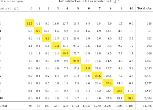
Before showing regression results, table 1 demonstrates the discrepancy in the outcome variables

yt_{t 1}1(life satisfaction referring to t-1 as reported in t-1) andyt_t 1(life satisfaction referring to t-1 as

reported in t). A cell entry is the percentage of those who reportyt_t 1, conditional on reportingy_tt 1₁

the plurality of observations record an answer consistent with the reported life satisfaction int 1

only for categories 5 (26%), 7 (30%), 8 (37%) and 10 (37%). All o¤-diagonal elements have positive

entries (excepty_tt 1 = 10_jy_tt 1₁ = 0), and people seem to “revise”their life-satisfaction both upwards

and downwards with a slight tendency for downwards revision: there are 5,675 observations in the

lower and 4,196 observations in the upper triangle of the table. The observations in the diagonal

cells are 4,202. This phenomenon lends strong support to the hypothesis of ‡exible thresholds

and/or the presence of a recall error.

Table 1: Cross-tabulations, Life satisfaction in %

LS in t-1 as repor- Life satisfaction in t-1 as reported in t: yt_t 1

ted in t-1: y_tt ₁1 0 1 2 3 4 5 6 7 8 9 10 Total obs

0 12.7 4.2 9.3 18.6 12.7 19.5 8.5 6.8 5.9 1.7 0.0 118

1 6.6 8.2 16.4 11.5 8.2 14.8 11.5 4.9 13.1 3.3 1.6 61

2 4.3 4.3 8.6 12.3 12.3 29.6 9.9 5.6 8.0 2.5 2.5 162

3 4.1 2.4 6.1 12.3 14.7 23.5 12.6 11.3 8.5 2.7 1.7 293

4 1.9 1.1 6.3 13.4 10.4 25.7 16.9 12.0 8.5 2.7 1.1 366

5 1.3 0.6 2.3 4.9 9.0 26.9 15.7 16.5 14.8 4.3 3.8 1,667

6 0.6 0.2 1.4 4.0 7.3 17.8 17.9 24.8 17.7 4.9 3.4 1,313

7 0.2 0.1 0.7 1.4 2.9 13.2 14.6 29.6 26.6 7.2 3.6 2,471

8 0.2 0.2 0.5 0.9 1.6 7.8 8.6 23.4 37.4 13.0 6.4 3,777

9 0.1 0.1 0.3 0.7 0.8 4.5 5.4 15.2 33.4 28.4 11.2 1,814

10 0.3 0.1 0.4 0.5 1.0 4.7 4.1 9.6 23.6 18.7 36.9 2,034

Total 95 55 183 357 536 1,723 1,495 2,782 3,721 1,726 1,403 14,076

Source: German Socio-Economic Panel 1984-1987. LS: Life satisfaction.

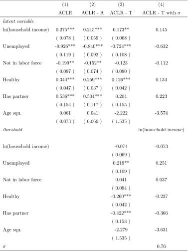
Table 2 presents results for our life-satisfaction model for the full sample, and compares it to the

ACLR estimator which is based on the current reported life-satisfaction only and to the alternative

Table 2: Life satisfaction determinants - Full sample

(1) (2) (3) (4)

ACLR ACLR - A ACLR - T ACLR - T with

latent variable

ln(household income) 0.275*** 0.215*** 0.173** 0.145

( 0.078 ) ( 0.059 ) ( 0.068 )

Unemployed -0.926*** -0.840*** -0.724*** -0.632

( 0.119 ) ( 0.092 ) ( 0.108 )

Not in labor force -0.199** -0.152** -0.123 -0.112

( 0.097 ) ( 0.074 ) ( 0.090 )

Healthy 0.344*** 0.259*** 0.126*** 0.134

( 0.047 ) ( 0.037 ) ( 0.042 )

Has partner 0.536*** 0.504*** 0.204 0.223

( 0.154 ) ( 0.117 ) ( 0.155 )

Age squ. 0.061 0.041 -2.222 -3.574

( 0.073 ) ( 0.060 ) ( 1.535 )

threshold ln(household income)

ln(household income) -0.074 -0.073

( 0.069 )

Unemployed 0.219** 0.251

( 0.109 )

Not in labor force 0.041 0.037

( 0.094 )

Healthy -0.260*** -0.237

( 0.042 )

Has partner -0.422*** -0.366

( 0.153 )

Age squ. -2.279 -3.631

( 1.535 )

0.76

Source: SOEP 1984-1987. All regressions include survey year dummies for the latent variable. For columns (1) to

(3) standard errors are clustered by individual and reported outcome (past vs. present). For column 4 standard

Not surprisingly, the results for in the ACLR model are roughly equal to in the ACLR

- T model. Minor di¤erences are due to missing values (for example iny_itt 1). As expected, we see

that important factors for reported life-satisfaction are income, good health, and employment. The

results suggest that accounting for threshold shifting variables can be quite important in practice.

In our preferred model (column 4) a third of the apparent increase in life-satisfaction through

income seems to be attributable to higher income shifting the threshold of what constitutes high

levels of life-satisfaction to the left. We had admittedly expected the opposite e¤ect. However, the

results also seem to suggest that the factors which increase (decrease) reported life-satisfaction (in

the ACLR model) have this dual e¤ect: they increase (decrease) the latent variable in our model,

but also shift the thresholds to the left (right). We see this phenomenon for all our variables except

age. We don’t want to read to much into such a parsimonious model, but a possible explanation is

that the things that constitute a good life might seem to be more easily attainable to people who

have it, while they might look distant and out of reach for those who lack it. Another important

point is that the ACLR - T model performs better than the ACLR - A model in terms of the Pseudo

R2 value. In the full sample this goodness of …t measure is 13% higher for the ACLR - T than for

the ACLR - A model. We view this …nding as supporting the remembered outcome speci…cation

we have proposed in this paper.

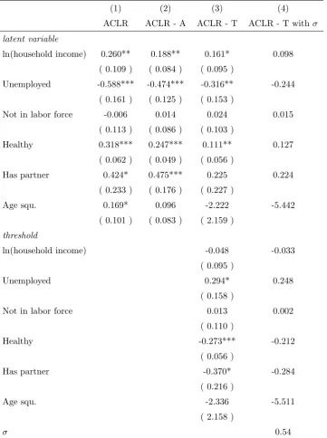
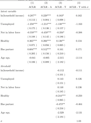
We are also interested in how income, unemployment and marital status a¤ect men and women

di¤erently and report results separated by sex in tables 3 and 4. Household income seems to

have comparable e¤ects on both men and women, though the e¤ect on the latent variable – the

emotional state –is smaller than the ACLR and ACLR - A models would suggest. An interesting

di¤erence exists with relation to employment status. Men are clearly much more negatively a¤ected

than women in their emotional state, while women seem to react to unemployment in part by

shifting out their thresholds. Not being in the labor force has no e¤ect on women, but a¤ects

men negatively. Presumably this is a life-style choice for women in that era, while for men

non-participation might re‡ect hidden unemployment or the inability to work. We also observe that

aging decreases women’s life-satisfaction strongly, but again women seem to “adapt” to this by

changing the thresholds, and by …nding it easier –for a given emotional state –to de…ne this state

as a relatively high level of life-satisfaction.

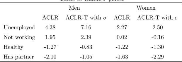
Important quantitative di¤erences also exist in the implied compensating incomes of conditions

like good or bad health or unemployment. We consider the dummy variables in our model in

table 5. The “shadow prices” in the model with ‡exible thresholds (columns 2 and 4) are based

on compensating incomes for incremental changes in the probability of switching from 0 to 1 in

the variable of interest. The shadow prices are based on changes in income to keep the latent

variable constant (rather than keeping the log odds-ratio constant). For example an increment

of 1 percentage point in the probability of getting unemployed is compensated by an increase

of 4.38% in the household income to keep the life-satisfaction of a man constant. In the ACLR

model no distinction between the e¤ect of a variable on the latent variable and the log odds-ratio

can be made. We see that for some variables the two models can imply very di¤erent shadow

prices. This is mostly clearly seen in the labor force variables, which according to our estimates

have higher shadow prices than the conventional ACLR model would imply. The not-in-labor-force

variable switches from positive to negative, though the di¤erence between the two estimates is not

statistically signi…cant. Finally, while the ACLR model suggests that having a partner is more

valuable for men than for women, this …nding is reversed in our ‡exible threshold model.

5

Conclusion

It has been a long-standing insight that in ordered-choice models there is an observational

equiv-alence between a variable’s e¤ect on the latent variable and on the threshold, and that only the

combined e¤ect is identi…ed. However, in practice the di¤erence between changes in the latent

variable and the threshold can be important for inference and policy-making. We are proposing

a model of ordered choice which accommodates the inclusion of 1) individual …xed e¤ects in the

Table 3: Life satisfaction determinants - Women

(1) (2) (3) (4)

ACLR ACLR - A ACLR - T ACLR - T with

latent variable

ln(household income) 0.260** 0.188** 0.161* 0.098

( 0.109 ) ( 0.084 ) ( 0.095 )

Unemployed -0.588*** -0.474*** -0.316** -0.244

( 0.161 ) ( 0.125 ) ( 0.153 )

Not in labor force -0.006 0.014 0.024 0.015

( 0.113 ) ( 0.086 ) ( 0.103 )

Healthy 0.318*** 0.247*** 0.111** 0.127

( 0.062 ) ( 0.049 ) ( 0.056 )

Has partner 0.424* 0.475*** 0.225 0.224

( 0.233 ) ( 0.176 ) ( 0.227 )

Age squ. 0.169* 0.096 -2.222 -5.442

( 0.101 ) ( 0.083 ) ( 2.159 )

threshold

ln(household income) -0.048 -0.033

( 0.095 )

Unemployed 0.294* 0.248

( 0.158 )

Not in labor force 0.013 0.002

( 0.110 )

Healthy -0.273*** -0.212

( 0.056 )

Has partner -0.370* -0.284

( 0.216 )

Age squ. -2.336 -5.511

( 2.158 )

0.54

Source: SOEP 1984-1987. All regressions include survey year dummies for the latent variable. For columns (1) to

(3) standard errors are clustered by individual and reported outcome (past vs. present). For column 4 standard

Table 4: Life satisfaction determinants - Men

(1) (2) (3) (4)

ACLR ACLR - A ACLR - T ACLR - T with

latent variable

ln(household income) 0.287** 0.229*** 0.163* 0.162

( 0.113 ) ( 0.084 ) ( 0.098 )

Unemployed -1.258*** -1.214*** -1.138*** -1.163

( 0.175 ) ( 0.136 ) ( 0.157 )

Not in labor force -0.559*** -0.459*** -0.356* -0.388

( 0.188 ) ( 0.145 ) ( 0.186 )

Healthy 0.365*** 0.266*** 0.136** 0.134

( 0.071 ) ( 0.056 ) ( 0.065 )

Has partner 0.604*** 0.512*** 0.161 0.171

( 0.205 ) ( 0.156 ) ( 0.210 )

Age squ. -0.041 -0.005 -2.315 -2.114

( 0.106 ) ( 0.089 ) ( 2.182 )

threshold

ln(household income) -0.112 -0.111

( 0.101 )

Unemployed 0.143 0.126

( 0.151 )

Not in labor force 0.148 0.136

( 0.185 )

Healthy -0.244*** -0.250

( 0.065 )

Has partner -0.473** -0.464

( 0.216 )

Age squ. -2.329 -2.131

( 2.184 )

1.03

Source: SOEP 1984-1987. All regressions include survey year dummies for the latent variable. For columns (1) to

(3) standard errors are clustered by individual and reported outcome (past vs. present). For column 4 standard

Table 5: Shadow prices

Men Women

ACLR ACLR-T with ACLR ACLR-T with

Unemployed 4.38 7.16 2.27 2.50

Not working 1.95 2.39 0.02 -0.16

Healthy -1.27 -0.83 -1.22 -1.30

Has partner -2.10 -1.05 -1.63 -2.29

Source: SOEP 1984-1987.

Crucially, our model can incorporate the same variables for the latent variable and the threshold

and identify their separate e¤ects. We apply our estimator to a simple model on life satisfaction

and demonstrate that variables usually included in life-satisfaction models have statistically and

quantitatively signi…cant e¤ects on the thresholds, which if omitted in the threshold speci…cation

are absorbed in the coe¢ cient of the latent variable speci…cation. Quantitatively important

di¤er-ences in the values of variables like unemployment, having a partner, health and not being in the

labor force arise between models with and without threshold shifts. Since our modeling strategy

depends on the availability of retrospective information on the dependent variable, we hope that

this paper will increase awareness for the importance of the inclusion of these variable in surveys.

References

Bago d’Uva, T. B., Lindeboom, M., O’Donnell, O., & Van Doorslaer, E. (2011). Slipping anchor?

Testing the vignettes approach to identi…cation and correction of reporting heterogeneity. Journal

of Human Resources, 46(4), 875-906.

Baetschmann, G., Staub, K.E. & Winkelmann, R. (2015). Consistent estimation of the …xed e¤ects

ordered logit model. Journal of the Royal Statistical Society: Series A (Statistics in Society),

forthcoming.

Chamberlain, G. (1980). Analysis of covariance with qualitative data. Review of Economic Studies,

Das, M. & Van Soest, A. (1999). A panel data model for subjective information on household

income growth. Journal of Economic Behavior & Organization, 40(4), 409-426.

Dolan, P., Layard, R. & Metcalfe, R. (2011) Measuring subjective wellbeing for public policy:

rec-ommendations on measures. Centre for Economic Performance special papers, CEPSP23. Centre

for Economic Performance, London School of Economics and Political Science, London, UK.

Dolan, P., Peasgood, T. & White, M. (2008). Do we really know what makes us happy? A review

of the economic literature on the factors associated with subjective well-being. Journal of economic

psychology, 29(1), 94-122.

Ferrer-i-Carbonell, A. & Frijters, P. (2004). How Important is Methodology for the estimates of

the determinants of Happiness? The Economic Journal, 114, 641-659.

Haisken-DeNew, J.P. & Frick, J.R. (2005). Desktop Companion to the German Socio-Economic

Panel, Version 8.0. Available athttp://www.diw.de/documents/dokumentenarchiv/17/38951/

dtc.354256.pdf

Hamermesh, D.S. (2001). The changing distribution of job satisfaction. Journal of Human

Re-sources, 36, 1-30.

Her Majesty’s Treasury Budget (2010). Available from: http://www.direct.gov.uk/prod_

consum_dg/groups/dg_digitalassets/@dg/@en/documents/digitalasset/dg_188581.pdf

Lindeboom M. & van Doorslaer E. (2004). Cut-point shift and index shift in self-reported health.

Journal of Health Economics, 23, 1083-1099.

Mukherjee, B., Ahn, J., Liu, I., Rathouz, P.J. & Sánchez, B.N. (2008). Fitting strati…ed

propor-tional odds models by amalgamating condipropor-tional likelihoods. Statistics in Medicine, 27, 4950-4971.

Organisation for Economic Co-Operation and Development (2011). How’s life?

Measur-ing well-beMeasur-ing. Available from: http://www.oecd-ilibrary.org/economics/how-s-life_

Terza, J.V. (1985). Ordinal probit: a generalization, Communications in Statistics - Theory and

Methods, 14, 1-11.

Winkelmann, L. & Winkelmann, R. (1998). Why are the unemployed so unhappy? Evidence from