City, University of London Institutional Repository
Citation
:
Yezzi, A. J., Slabaugh, G. G., Broadhurst, A., Cipolla, R. and Schafer, R. W.
(2002). A Surface Evolution Approach to Probabilistic Space Carving. In: First International
Symposium on 3D Data Processing Visualization and Transmission, 2002. Proceedings. (pp.
618-621). IEEE Computer Society. ISBN 0-7695-1521-5
This is the accepted version of the paper.
This version of the publication may differ from the final published
version.
Permanent repository link:
http://openaccess.city.ac.uk/4395/
Link to published version
:
http://dx.doi.org/10.1109/TDPVT.2002.1024126
Copyright and reuse:
City Research Online aims to make research
outputs of City, University of London available to a wider audience.
Copyright and Moral Rights remain with the author(s) and/or copyright
holders. URLs from City Research Online may be freely distributed and
linked to.
City Research Online:
http://openaccess.city.ac.uk/
[email protected]
A Surface Evolution Approach to Probabilistic Space Carving
Anthony Yezzi, Greg Slabaugh
School of Electrical and Computer Engineering
Georgia Institute of Technology
Adrian Broadhurst, Roberto Cipolla
Department of Engineering
University of Cambridge
Ron Schafer
School of Electrical and Computer Engineering
Georgia Institute of Technology
Abstract
We present a 3D photography method that generates a texture-mapped three-dimensional model of a scene com-puted from multi-view calibrated two-dimensional pho-tographs. Our approach first performs probabilistic space carving, which results in a 3D grid of voxel probabilities that describe the likelihood of a voxel existing in the model. We then employ a three-dimensional geodesic active sur-face to extract a most likely conformally-weighted minimal surface from the voxel probabilities. This surface is then polygonalized and texture-mapped, yielding in a 3D model easily rendered with standard graphics hardware.
1. Introduction
The objective of this work is to reconstruct a three-dimensional shape from a set of two-three-dimensional images in a formal statistical manner through the use of a geometric active surface model which allows us to easily incorporate geometric smoothness constraints.
We begin with an array of voxels where each voxel is as-signed a probability of existing in the reconstructed shape. In addition, each voxel is assigned a spherical Gaussian color distribution. Thus when a voxel is projected onto an image, the color of each resulting pixel is a sample point drawn from that voxel’s color distribution. This is a useful model because a voxel will often project to several pixels per image and this assumption does not require all of these image pixels to have identical RGB values.
This approach differs from Space Carving [7] because each voxel is assigned a probability for it existing in the model. This probability may be regarded as a continuous measure of photo-consistency. Since this measurement is non-negative, it is naturally used as a weighting factor in the framework of geometric active surface models. Specifi-cally, our goal will be to seek a closed 3D surface of
mini-Table 1.Notation used in this paper.
Indices
i Image index∈ {1. . . n}
x, y Pixel co-ordinate index
k, l, m Voxel index (mis depth)
Image data
Ii ImageIi Ii
xy Pixelx, yof imageIi
Ri An image region within imagei Ri
klm Region ofIiprojected byklm
Geometric variables
Pi Projection matrix for imageIi
Hi
m Homography from planemtoIi
Statistical variables
D All available data{{Ii},{Pi}}
∃klm ∃klm∈ {0 =empty,1 =exists} Vklm The model for a voxel atklm
Wi
klm The missing voxel model for imagei
Gaussian parameters
µ=(µRµGµB) Gaussian mean in RGB space
σ2
R, σG2, σ2B Gaussian variance in RGB space
mal area but where the local area element on the surface is weighted in inverse proportion to the probabilities assigned to the nearby voxels. In this manner, the surface will be attracted to more photo-consistent locations within the 3D grid (since smaller weighted areas arise at such locations) while remaining smooth as well.
[image:2.595.309.548.278.526.2]proba-bilistic measure of photo-consistency. This surface can then be polygonalized and texture-mapped, producing a model well suited to rendering with standard graphics hardware.
2. Computing Voxel Probabilities
Consider pixel Ixyi which is located at co-ordinates
(x, y)in thei-th image. The probability thatIxyi is drawn from the spherical Gaussian distribution{µ, σ}is denoted
P(Ii
xy|µ, σ)and can be estimated using (1). P(Ixyi |µ, σ) = 1
σ√2π3e
− 1
2σ2Iixy−µ2 (1) Now consider the image region Ri which is the set of pixels{Ixyi }from imageIi. The probability that these pix-els are drawn from the distribution{µ, σ}can be calculated using (2). This probability is denoted P(Ri | µ, σ)and assumes that the image pixels are independent.
P(Ri|µ, σ)=
xy∈Ri
P(Iixy|µ, σ)=
xy∈Ri
e−
Ixyi −µ2
2σ2
σ√2π3 (2)
The next problem that needs to be discussed is the method used to decide whether or not a voxel should be part of the reconstruction. Each voxelklmprojects to a re-gionRiklm in imageIi. The image data in this region is described by one of two models. Either the data observed atRiklm is the result of the projection of a voxel, or it is described by some other feature in the reconstruction as the voxel is empty. The latter case is referred to as the case for the empty voxel. Bayes’ theorem is then used to determine which of the two cases is more likely, and is discussed in Section 2.3.
2.1. The statistical model for voxel projection
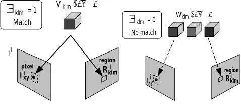
The first possibility is that the voxelklmis present in the reconstruction. This case is denoted∃klm= 1and is shown diagrammatically in Figure 1. In this case, the image data in regionRiklmis described by the statistical color distribution
Vklmof voxelklm, provided that the voxel is not occluded in this viewpoint. Remember, each voxel is represented by a spherical Gaussian distribution in RGB space. This means that Vklm has four degrees of freedom that need to be es-timated, which are {µR, µG, µB, σ2} (see Table 1). The probability that the observed data in imageIiis described by the voxel modelVklmis obtained by considering the pix-els in regionRiklmand is denotedP(Ii| ∃klm=1,Vklm).
P(Ii|∃klm=1,Vklm)=P(Riklm|µ, σ)=
xy∈Ri klm
P(Ixyi |µ, σ) (3)
Equation (3) gives the probability for the data observed in one particular image, given that the voxel exists in the
Ii
={µ,σ} klm
V
klm = 1
i xy
I Rklm
i region pixel
Match klm={µ,σ}
Wi klm= 0
[image:3.595.308.547.73.176.2]klm Ri xy Ii 000 000 000 000 000 000 000 111 111 111 111 111 111 111 000 000 000 000 000 000 000 111 111 111 111 111 111 111region No match
Figure 1. The models for the projection of a voxel (left) and for a missing voxel (right).
reconstruction. The combined probability for observing all of the images can be calculated by assuming that each of the images is independent.
P(D|∃klm=1,Vklm) =
i
P(Ii|∃klm=1,Vklm) (4)
Unfortunately, the parameters of the voxel modelVklm are not known, so they have to be marginalized1 by
inte-grating over all possible values for the distribution.
P(D|∃klm=1) =
Vklm
P(D|∃klm=1,Vklm)P(Vklm)dVklm (5)
The prior termP(Vklm)is a distribution that describes the model parameters ofVklm(see [2, 1] for details).
2.2. The statistical model for an empty voxel
The second possibility is that the voxelklmdoes not ex-ist. This case is denoted∃klm = 0and is shown in Figure 1. In this case, the non-voxel is projected into each of the images, and the image samples that are obtained are pro-jections of different voxels. Unfortunately, it is not known which voxels these are until the entire scene has been recon-structed. To get around this difficulty, the voxel projections
Ri
klm are assumed to be locally independent. This means
that a missing voxel can be represented by a set of indepen-dent statistical models{Wklmi }, one for each image. Again, each of these models is represented by a spherical Gaussian
{µR, µG, µB, σ2}distribution.
The probability that the observed data in imageIiis de-scribed by the voxel modelWklmi is obtained by consider-ing the pixels in regionRiklm.
P(Ii|∃klm=0,Wklmi )=P(Riklm|Wklmi )=
xy∈Ri klm
P(Ixyi |µ, σ)
(6)
1To marginalize a parameter using Bayes’ rule, integrate over all
pos-sible values for the parameter, multiplied by the prior at that value, and divide by the total probability.
Since the specific value of Wklmi is not known, it is necessary to marginalize this parameter by integrating over all possible values of Wklmi multiplied by the prior term
P(Wi
klm). This prior term describes the distribution of the
model parameters ofWklmi (see [2, 1] for details).
P(Ii|∃klm=0) =
Wi klm
P(Ii|∃klm=0,Wklmi )P(Wklmi )dWklmi
(7)
Equation (7) calculates the probability of the data in a particular image given that it is the result of an independent voxel. This probability can be calculated for each of the images independently and the combined result is given by:
P(D| ∃klm= 0) =
i
P(Ii| ∃klm= 0)
=
i
Wi klm
P(Ii|∃klm=0,Wklmi )P(Wklmi )dWklmi
(8)
Visibility can be addressed by analyzing the existence of voxels along a ray between voxelklmandIi, as described in [2, 1].
Two probabilities have now been calculated. The first is the probability of the image data given that it is described by a single voxel (5). The second is the probability of the image data given that it is described by the projection of independent voxels (8). The final step is to calculate which of these two cases is more likely.
2.3. How to make a decision about a voxel
The probability of a voxel existingP(∃klm= 1| D)is determined using Bayes’ Theorem from the probabilities of the two possible voxel models. These are the model for a voxel existingP(D| ∃klm= 1), and the model for a voxel being empty P(D | ∃klm = 0). The prior probabilities for a voxel existing, or not existing, are denoted: P(∃=
1) +P(∃= 0) = 1. These probabilities can be combined using Bayes’ Theorem:
P(∃klm= 1|D) =
P(D| ∃klm= 1)P(∃= 1)
P(D|∃klm=1)P(∃=1) +P(D|∃klm=0)P(∃=0) (9)
3. Computing the 3D Surface
The result from the previous section of this paper is a volume of probabilities. Now we want to use these proba-bilities to find a most likely reconstructed surfaceS. Fol-lowing the same intuition as Faugeras and Keriven [5] us-ing the 3D extension of geodesic active contours [3, 11], we will use our probabilistic measure of photo-consistency
to non-uniformly weight the standard Euclidean metric of the volume space by a conformal factorΦ, and then seek a minimal surface (surface of least area) where its area is measured according to this conformally weighted metric. Faugeras and Keriven did not employ such a probabilistic measure but used normalized cross correlation measures as their weighting factor instead.
In particular, the surfaceSwill be chosen to minimize
E(S) =
SΦdA
where Φ = 1
1 +P(∃klm=1|D) (10)
by starting with an initial guess forSand then deforming it via the following gradient flow
∂S
∂t = ΦH N−(∇Φ·N)N (11)
whereH denotes mean curvature and N the inward unit normal toS. Intuitively, regions that locally are low prob-ability will haveΦ ≈ 1 and∇Φ ≈ 0. In such a region, the first term in equation 11 dominates, and the surface
S smooths via evolution by its mean curvature. For re-gions that locally are high probability, the second term in equation 11 dominates, and the surface S flows towards and locks onto local maxima of the computed probability
P(∃klm= 1|D). For other values of probability, there is a balance between these two terms.
We use level set methods of Osher and Sethian [8] to implement this flow since they allow easy handling of topo-logical changes, since the surface S might need to break apart into multiple nearby pieces during evolution. When the flow is complete, the surface S can be extracted from the level set function using the Marching Cubes [6] algo-rithm, resulting in a polygonal representation that is eas-ily texture-mapped using the original photographs and ren-dered in graphics hardware.
4. Experiments
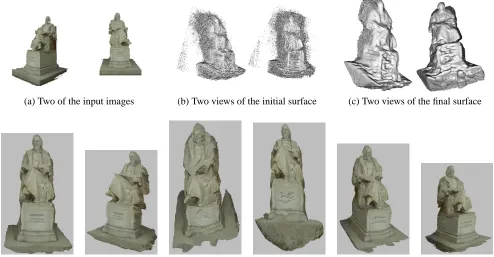
The steps of this algorithm are illustrated in Figure 2. Two images of the Lord Tennyson statue are shown in Fig-ure 2a (after segmenting away the background). The com-puted voxel probabilities are then examined with some sim-ple heuristics to derive an initial estimate of the surface. Two views of the initial surface are shown in Figure 2b. This gives a rather poor reconstruction since no notion of geo-metric smoothness has been incorporated into the Bayesian probability estimates. Next, in Figure 2c we see the final re-constructed surface obtained by evolving the initial surface in Figure 2b via the flow of equation 11. Finally, in the bot-tom row of the figure we see six different views of the final reconstruction after texture mapping the original image data onto the result in Figure 2c.
(a) Two of the input images (b) Two views of the initial surface (c) Two views of the final surface
Figure 2. Reconstruction of Lord Tennyson statue. The top row shows two of the input images followed by views of the initial and final surface. The bottom row shows many more views of the final reconstruction with texture mapping of the original image data.
guess forSwas not near a maxima, the gradient term would have little influence on the surface evolution, and the sur-faceS would not move towards the maxima. To address this issue, we implemented a diffusion of the gradient field using the technique of Xu and Prince [10]. We compute this gradient field diffusion by solving a set of decoupled partial differential equations. This is performed before the surface evolution of equation 11.
5
Conclusion
We have presented a method for computing a 3D model of a scene using multiple 2D photographs. Our technique employs a probabilistic framework for space carving and a geodesic active surface model for extracting a smooth, most likely surface.
References
[1] A. Broadhurst. A probabilistic framework for the Space
Carv-ing algorithm. PhD thesis, University of Cambridge, Dept. of
Engineering, 2001.
[2] A. Broadhurst, T. Drummond, and R. Cipolla. A probabilistic framework for the Space Carving algorithm. In Proc. ICCV, pp. 388–393, Vancouver, Canada, July 2001.
[3] V. Caselles, R. Kimmel, G. Sapiro, “Geodesic snakes,” Int. J.
Computer Vision, 1998.
[4] B. Culbertson, T. Malzbender, and G. Slabaugh. Generalized voxel coloring. In B. Triggs, A. Zisserman, and R. Szeliski, editors, Vision algorithms: Theory and Practice, volume 1883 of Lecture Notes in Computer Science, pages 100–115, Corfu, Greece, Sept. 1999. Springer-Verlag.
[5] O. Faugeras and R. Keriven. Variational principles, surface evolution, PDEs, level set methods, and the stereo problem.
Tran. on Image Processing, 7(3):336–344, March 1998.
[6] W. Lorensen and H. Cline. Marching Cubes: A High Reso-lution 3D Surface Construction Algorithm. In SIGGRAPH, pages 163–170, 1997.
[7] K. Kutulakos and S. Seitz. A theory of shape by space carv-ing. Int. J. Computer Vision, 38(3):198–218, July 2000. [8] S. Osher and J. Sethian. Fronts propagating with
curvature-dependent speed: algorithms based on Hamilton-Jacobi equa-tions. J. of Comp. Physics, 79:12–49, 1988.
[9] S. Seitz and C. Dyer. Photorealistic scene reconstruction by voxel coloring. Int. J. Computer Vision, 35(2):1067–1073, 1999.
[10] C. Xu and J. Prince, “Snakes, Shapes, and Gradient Vector Flow”, IEEE Trans. Image Processing, 7(3):359–369, March 1998.
[11] A. Yezzi, S. Kichenassamy, A. Kumar, P. Olver, and A. Tan-nenbaum, “A Geometric Snake Model for Segmentation of Medical Imagery”, IEEE Trans. Medical Imaging, vol. 16, no. 2, pp. 199–209, 1997.