Vibration-based methods for structural and machinery fault diagnosis based on nonlinear dynamics tools

Vibration-based Methods for Structural and Machinery

Fault Diagnosis Based on Nonlinear Dynamics Tools

Emil Manoach Department of Applied Mechanics Lublin University of Technology, Lublin, Poland Institute of Mechanics, BAS, Bulgaria

1.

Introduction

Monitoring the condition and the health of structures and machinery is one of the first priorities in a proper maintenance program. The reasons for this are multiple and include (but are not restricted to) the safety and the reliability of the structure as well as economical ones.

Vibration-based health monitoring (VHM) methods are quite popular and are of extensive use for monitor-ing structures as well as machinery. The meanmonitor-ing of such approaches is that practitioners look for features de-rived from vibration signals measured on a structure or machinery that ostensibly change as the struc-ture’s/machinery dynamics change due to some degradation or failure mechanism. Thus the vibration response of a structure/machine can be used to monitor its condition and to detect and diagnose faults in it. A lot of dif-ferent methods have been proposed to extract features from a vibration signal that can be used for certain fault diagnosis purposes. These damage features should be sensitive to the initialization and the growth of a certain fault type and in the same time they should be robust to noise and other factors like noise, temperature and operational/environmental conditions. Features can be extracted from the time domain and/or the frequency domain of a signal as well as from the modal domain of a structure/machine. Vibration-based methods are global non-destructive monitoring methods and as such they can be used for detecting faults in parts of the structure that are difficult or impossible to access.

reasons for using phase space is that nonlinear signals are slightly predictable in time, but they have structure which can be observed in a phase space. The dynamic response of a nonlinear system may look random in the time and in the frequency domain, but it has order and shape in a phase space. A frequency representation of a vibrating system will have thousands of frequency components while in the state space we are following the trajectories of the system which would converge to an attractor. An example is shown on Figure 1 below which gives the time history, the spectrum and the phase diagram of the vibration response of a circular plate which is subjected to a frequency equal to its first natural frequency.

0 0.02 0.04 0.06

t , sec. -0.2

-0.1 0 0.1 0.2

w

/R

(a) (b)

(c)

Figure 1: Time history a), spectrum b) and phase diagram c) of an aluminum circular plate with ra-dius R=0.1 m and h=0.01m subjected to harmonic loading with amplitude 1500 kN uniformly dis-tributed along the plate surface, excitation frequency equal to the first natural frequency (ωe = 15300

Rad/s)

Attractor-based methods for structural health monitoring were introduced and explored first by the authors of (Olson et al 2005, Moniz et al 2003, Moniz et al 2005, Nichols et al 2003,2004,2005,2006,Todd et al 2001, 2004) as well as by the authors of the present study (Trendafilova et al 1999, 2000,2001, Trendafilova 2002,2003, Trendafilova & Manoach 2008). In (Moniz et al 2003, Nichols et al 2003004,2005,2006,Olson et

V35-IR1.DAT

Fourier Frequency Spectrum

833.55 935.2 1037.3

1138.5 1455.8

1659.4 2180.4 2801.9 4050.3

0 50000 1e+05 1.5e+05 2e+05 2.5e+05

Frequency -100

-75 -50 -25 0 25 50 75

dB

-100 -75 -50 -25 0 25 50 75

dB

-0.2 -0.1 0 0.1 0.2

w/R

-200 -100 0 100 200

D

im

e

ns

io

n

le

ss

v

e

lo

ci

al 2005) the authors explore the possibility of exciting the structure with chaotic signal which results in nonlin-ear/chaotic response. The authors of this study use random and/or large amplitude vibrations to excite structural nonlinearities. The advantage of using random (ambient) excitation is that this is the natural source of excita-tion for most structures. Harmonic excitaexcita-tion is easier to produce and apply to a structure rather as compared to a chaotic one.

Most state-space methods exploit the reconstructed attractor to extract damage sensitive features. There are two possibilities: to compare the attractors of the healthy and the damaged structure or the attractors built from data measured in different points (Olson et al 2005, Trendafilova 2006). The attractors can then be compared on the basis of different features. Since attractors are sets of points (data sets) in the state space one possible way to characterise them is by using statistical methods and characteristics. This approach was followed by the authors of the present study (Trendafilova 2003,2006,Trendafilova &Manoach 2008) and some of the follow-ing paragraphs explain the application of several such possibilities for damage feature extraction. The authors of (Todd et al 2001,2004) also explore several such possibilities. These type of methods have the advantage that in general the characteristics that they use can be estimated following existing statistical procedures and in this sense they are easily extractable form data. A disadvantage might be that these characteristics depend on the quantity and the quality of the data available. Most of these characteristics extracted from the data set of the attractor show quite good performance in the sense of sensitivity to damage and noise insensitivity (Torkamani 2011, Trendafilova 2006, Nichols et al 2005, Olson et al 2005). The other possibility is to use the invariants of the reconstructed attractors e.g. Lyapunov exponents and/or state space dimensions. This approach has been followed in e.g.(Olson et al 2005, Moniz et al 2005) as well as by the current authors (Trendafilova 2006, Trendafilova& Van Brussel 2001). The invariants are characteristics of the dynamic system and they are inde-pendent on the state space in which it is represented. These methods also show quite good sensitivity to dam-age while in the same time being insensitive to noise as well as to changes in the reconstructed the attractor (Olson et al 2005, Trendafilova 2006). The problem with such methods is that the invariant characteristics of the state space and the attractor are quite difficult to estimate from data and thus the obtained estimates should be considered to possess quite some variability/uncertainty.

A somewhat different approach followed in (Todd et al 2004, Nichols et 2003), is the method of prediction error. The reconstructed attractor is used to build predictive models of the system dynamics and the prediction error is then used as an indicator for damage .The general principle is to follow the evolution of local neigh-bourhoods of trajectories on the attractor and use the evolved neighbourhood to make a prediction. Again the attractors of the healthy and the damaged structure can be compared as well as the attractors built from differ-ent measuremdiffer-ent points. The difference is that rather than using characteristics of these attractors, predictive models are built and it is hypothesised that a prediction error will increase with damage.

This study explains and demonstrates the utilisation of different nonlinear-dynamics-based procedures for the purposes of structural health monitoring as well as for monitoring of robot joints.

2.

The Phase (state) Space Approach

In this paragraph we introduce the basics of the phase-state approach and how it can be used for structural and machinery dynamic/vibration modelling.

2.1. The Main Idea of the Phase-State Methodology

x _=F(x(t))

dt

d ₍₁₎

In most cases the function F(.) in the above model is not explicitly known and the original system space defined by the vector x is also unknown. Any dynamic system can be completely unfolded in its phase space, where the trajectories of the system converge to an invariant subspace (the attractor). The question is how to reconstruct this space especially for cases when there is not enough a priori information available about the system and one is able to observe only one or two variables. Obviously a vibrating structure or a rotat-ing/moving machinery is a much more complex system and cannot be represented in a one-dimensional space. Takens theorem (Abarbanel, 1996) gives the answer to this question. The theorem tells that if we are able to observe a single scalar quantity s(n), n=1,2…. of some vector function of the dynamic variable x,

))

(

(

(

)

(

n

s

n

s

=

g

x

n=1,2,..,m, with components consisting of s(n). The vectors y(n):

y(n) = [s(n), s(n + T),…, s(n + m – 1) T] (2)

composed simply of time lags of the observation define the motion in an m-dimensional Euclidean space. In

particular it is shown that the evolution in time of the points y(n) y(n + 1) follows that of the unknown

dy-namics x(n) x(n + 1). This procedure converts the scalar measured series s(n) into a series of vectors y(n).T

and m are properly chosen time delay and dimension respectively. They are known as the embedding

parame-ters of the new state space. The choice of proper embedding parameparame-ters is outside the scope of this paper and is discussed in detail for example in (Abarbanel,1996, Krantz & Schreiber,1997). Here we only mention how these parameters can be obtained.

The time lag T is chosen so that the consecutive measurements in the moments t and t+T are independent

from viewpoint of information but not so independent that information is lost. The first minimum of the

aver-age mutual information (AMI) is used to determine the time lag T (Krantz & Schreiber,1997) . The AMI is

used as a measure of correlation between two measurements. The time lag is determined so that two consecu-tive measurements are far enough from each other to be useful as independent coordinates but not too far to have no connection with each other (Abarbanel,1996, Fraser & Swiney,1986).

A proper embedding dimension is needed to “unfold” the dynamics of a system. The false nearest neigh-bour approach can be used for the purpose (Abarbanel,1996, Krantz & Schreiber,1997). The idea of this meth-od is that the percentage of false nearest neighbours should become 0 when the adequate minimum unfolding dimension is reached.

2.2. How Does the State-Space Representation Method Work

Now that we have reconstructed our new phase space which is made of the vectors y(n) constructed according to (2), we want to represent our system in this new space.

According to the traditional dynamics approach (which is in fact appropriate for systems which are linear or with behaviour close to linear) a dynamic/vibrating system can be represented in its time domain, in its fre-quency domain or in its modal domain. The time domain representation consists of a signal or an ensemble of measured signals as a function of the time t. The frequency domain representation of a system is given by the Fourier transforms of the ensemble of the initial signals. For a nonlinear dynamic system the time domain as well as its frequency domain representations might look random which might make it difficult or even impos-sible to extract useful information from these representations. From Figure 1 it can be seen that it is difficult to extract information from these two representations. While on the contrary the phase-space diagram represents a much more ordered image which is easier to analyse visually. Regarding the modal representation it should be mentioned that in general these cannot be obtained for a nonlinearly vibrating system. Thus the phase space representation looks like the best alternative for a nonlinear dynamic/vibrating system.

The phase space is a space in which all possible states of a system are represented, with each state corre-sponding to one unique point in the phase space. For a two dimensional space the phase space is usually made of the position /displacement and its time lag/ momentum. A phase space diagram represents all possible dy-namic states of a structure in a two-or three dimensional space. In a phase space, every degree of freedom of the system is represented as an axis of a multidimensional space and for every possible state of the system a point is plotted in the multidimensional space. This succession of plotted points is analogous to the system's state evolving over time. In the end, the phase diagram represents all that the system can be, and its shape can easily elucidate qualities of the system that might not be obvious otherwise. Thus the phase space allows to observe features of the dynamics of a system which cannot be observed in any of its other representations.

3.

The Phase/State Space Approach for Health Monitoring of Structures and

Ma-chinery.

One way to characterize the dynamics of a system in a state space is by reconstructing the mapping relation:

y (t + T) = G(y(t)) (3)

Unfortunately for most dynamic systems the evolution relation (3) is not available. The Fourier analysis of the motion of many nonlinear systems will lead to a continuous spectrum, which is associated with an infinite number of modes. Nonlinear dynamics suggests a more general approach to study the dynamics of a system in

its phase space, vis. by studying its attractor, which can be characterized by its invariants- the Lyapunov

spec-trum, the entropy and different dimensions. It can be argued and there is much evidence that these characteris-tics change with the introduction of damage (Hunter al 2000, Todd et al 2001, Trendafilova 2002, Trendafilova 2003, Moniz et al 2005). The Lyapunov spectrum of a dynamic system characterises the average rate of con-traction or expansion in each of the principal geometric directions of the state space. For a linear vibrating sys-tem the Lyapunov exponents are determined by the real parts of the eigen values of the state space matrix of the system. Since it is clear that many damage scenarios affect the eigen state of a structure (Brincker et al,1994, Hunter et al,2000) then it can be argued that damage will affect the Lyapunov spectrum of a vibrating structure and hence – the geometry of its state space. Some of our and other authors’ research has shown, and it has been experimentally confirmed, that the Lyapunov exponents and the geometry of the attractor of a vibrat-ing system not only change under the introduction of damage, but they are rather sensitive to different kinds of damage (Todd et al,2001, Nichols et al 2003, Trendafilova 2002, Trendafilova 2003, Craig et al 2000). Unfor-tunately these invariants are on a lot of occasions are rather difficult to estimate precisely enough from data. There are methods for their estimation but they offer somewhat approximate results which on some occasions might be quite erroneous and might somewhat differ from the real invariants. This can be considered as a dis-advantage when using these invariants for damage/fault isolation purposes.

distribution or by approximating the distribution function. This may be considered as a much better alternative as compared to the invariants estimation because these characteristics are quite easy and straightforward to estimate from data.

The two approaches for characterizing a dynamic system introduced above are closely related and can be considered identical since they are linked by the ergodic theory (Eckmann &Ruelle 1985). The ergodic theorem asserts that time averages are equal to space averages. One of the virtues of the ergodic theory is that it allows consideration of the long term behaviour of a system. Since the physical long term behaviour of a dynamic system is on the attractor the system is thereby characterized by its attractor. The ergodic theory permits the invariants of a dynamic system to be viewed as invariant statistical quantities of the attractor.

Another possibility to characterize a dynamic system for the case of periodically driven oscillators is to uti-lize its Poincaré map. The Poincaré map is a projection of the phase diagram for a moment t, which is a multi-ple of the period of the system. It has been suggested by the authors of this chapter as a possible feature for damage detection in structures.

The methods considered in this paper explore the three possibilities introduced above. The next sections in-troduce the application of the Poincaré map (&3.1) and the distribution of state space points (&3.2) for damage diagnosis. &3.3 offers an example for the application of these two methodologies. The application of phase space invariants for damage/fault assessment in structures is discussed in (&3.3).

3.1. The Poincaré Maps and their Application to Structural VHM

A standard technique for dealing with phase space (w, w, t) of periodically driven oscillators is to study the

projection of (w, w) at moments in time t, where t is a multiple of the period T=2π/ω. Here ω can be the

fre-quency of the excitation of the mechanical system, an eigen-frefre-quency of the structure, or its multiple, and T is

a period of the forcing function, an eigen-period of the system, or its multiple. The result of inspecting the

phase projection (w, w) only at specific times t=kT is a sequence of dots, representing the so-called Poincaré

map. The steady-state converging trajectories, which represent the attractor, are usually formed in the phase space and in many cases of nonlinear systems they are very sensitive to any changes in the system.

A Poincaré map can be interpreted as a discrete representation of the dynamic system in a state space which is one dimension smaller than the original continuous space of the dynamic system. Since it preserves many properties of periodic and quasi-periodic orbits of the original system and has a lower dimension, it is often used for analyzing the original system.

Only a few authors have checked the influence of a fault on the Poincaré maps of the system (Choy et al 2009, Choy et al 2007, Choy et al 2007)

In the authors’ papers (Manoach&Trendafilova 2008, Trendafilova&Manoach 2008) for the first time a damage index based on analysing the Poincaré maps of structures is introduced. According to these papers the damage index for each mode (i) of the discretized structure is:

u i

d i u i P i

S S S

F = − ,

𝑆_!!_{= 𝑤}

!!,!!!−𝑤!!,!

!

+ 𝑤_!!_,!!!−𝑤

!!,!

!

!!!!

!!! (4)

𝑆_!! _{= 𝑤}

!!,!!!−𝑤!!,!

!

+ 𝑤_!!_,!!!−𝑤

!!,!

!

!_!!!

!!!

where, i =1 , 2…Nnodes , Nnode is the number of nodes, Np is the number of points on the Poincaré map and (wij,

wij) and (wij, wij) denotes the jth point on the Poincaré maps of the undamaged and the damaged states,

respec-tively.

The damage index suggested by eq (4) represents the relative difference between the lengths of the curves formed by connecting the dots on the Poincaré maps for the non-damaged and the damaged plate for ith node, respectively. This difference is accepted as a measure for the global change (during of the total period of

vibra-. .

.

. d . d

u

tion) in the dynamic behaviour of the damaged structure in comparison with the undamaged one. The assump-tion is that if the funcassump-tion FP(x) has maximum and it is strongly concave in the vicinity of the maximum, the structure has damage and the nodes close to the maximal value of the function will represent the damaged area.

The above damage index depends on the location of the damage in the structure, and consequently it is a function of the structure coordinates X(x1,x2,x3). One can expect that the maxima of the function FP(Xd) will

represent the locations of the damage, i.e. Fmax(Xd) =max{Fi }.

The Poincaré maps contain data for the displacements and the velocities of the structure in a compact form and since these two parameters are expected to be sensitive to damage these diagrams can be used to detect damage. When the damage is large and the plate undergoes substantial nonlinear vibrations, this leads to changes in the attractor of the vibrating system in the phase space and then the application for damage assess-ment purposes becomes obvious. Even when the damage is small, and the responses of the damaged and the healthy structure are close to each other, the points from the Poincaré map are easier to use for comparison and identification purposes because the number of these points is much smaller than the enormous number of points in the time-history diagrams.

It is logical to expect that at the nodes close to the damaged area the introduced damage index FiPwill be

larger than the index for points which are far from the damaged zone. This can be used to localize the detected damage.

So the damage criterion can be formulated as:

FP(X) > Td (5)

where X is the vector of the space variables and Td _{is the threshold for the damage index.}

It should be mentioned that this threshold is case dependent and it depends on the structure tested, the envi-ronmental conditions, as well as on the characteristic used as a damage feature.

3.2. Statistical Distribution of Points on the Attractor And The Effect of Damage on It.

This method suggests to study the statistical distribution of points on the attractor and use it to extract damage sensitive features. In contrast to the previous method it can be used for any type of excitation including random one which is the natural source for most structures. An advantages of using these statistical characteristics is that they are easy to determine from measured data. Another advantage is that in general the statistical charac-teristics of a nonlinear system are more robust to noise than any deterministic characcharac-teristics. The determina-tion of any deterministic characteristics (invariants) of a nonlinear signal from observadetermina-tions is very difficult (if possible at all) and the estimated characteristics could be quite imprecise (Abarbanel,1996, Krantz & Schreiber,1997).

As it was mentioned above, a two-dimensional state space is used in this investigation. The time lag ΔT

was found using the first minimum of the average mutual information in order to generate a number of “uncor-related” points in the state space (Abarbanel,1996, Krantz & Schreiber,1997, Fraser & Swiney,1986). To study the attractor one needs a long enough signal which will exclude the transient and short term behaviour and allow one to concentrate on the long term behaviour of the system. For a vibrating system one measures accel-eration, velocity or displacement signals. Any of these quantities can be used to obtain a sample of state space points. For the purposes of this method we use acceleration signals only because acceleration is the most com-mon quantity to measure on a vibrating structure. Suppose one measures a long enough acceleration signal. It

can be represented by an acceleration vector a as follows:

n i T t t a a a t a t a t a i i T n T n ,..., 3 , 2 ] ,..., , [ )] ( ),...., ( ), ( [ 1 2 1 2 1 = + = = = − a (6)

where a(ti) are the measured accelerations in the time moments ti,i=1,2….,n,n is large enough, the superscript

[…]T _{stands for transpose and T is the time lag found as explained above.}

From a vector a one can obtain n-1 state space points:

y_i= [y_i1, y_i2]T _{= [a}

i, ai+1]T, i = 1, 2, … n-1 (7)

A set of N trajectories y_k, k = 1, 2, …N, is then randomly chosen on the response attractor and N_B nearest

neighbours are found for each trajectory in the sense of Euclidean distance, yi

q, i=1,2,…,N,q=1,2,…NB. This

set is denoted by Yn,

⎭ ⎬ ⎫ ⎩ ⎨ ⎧ = = = N k N q k q n B ,... 2 , 1 ,... 2 , 1 y

Y . The set Yn, n = 1, 2, …, N. NB = M is used to characterise the

attrac-tor of the response signal.

Now that we have obtained the set of vectors Yn the next task is to characterise the statistical distribution of

these points. One way to do this is to estimate some statistics of the obtained sample Yn. Some of our and other

authors’ previous research has shown that certain statistical characteristics of this distribution might be sensi-tive to damage (Todd et al 2001, Sohn & Farrar,2001, Trendafilova,2006, Trendafilova,2003, Matthew,1997). For instance the variance and the skewness have been found to show sensitivity to damage in some cases, while other statistical moments turned less sensitive (Todd et al 2001, Nichols et al 2004, Trendafilova,2006). For a multidimensional distribution the variance and the skewness can be defined by the following scalar quantities, respectively (Mardia 1970):

∑ ∑ − − = ∑ ∑ − − = = = = = n i n j T n i n j T M s M 1 3 1 2 1 2 1 2 )] ) [( 1 )] ( ) [( 1 Y (Y S Y Y Y Y S Y Y j i j i σ (8)

where M is the number of points Y_n, n=1,...,M, Yis the sample mean vector and S is the sample covariance

matrix. Instead of using the values for σ and s one can introduce relative changes compared to the non

dam-aged case. These characteristics are introduced below:

n n s n n s s s F F − = − = σ σ σ σ (9)

The above quantities can be used as damage features/indexes. The multivariate statistics (8) as well as the damage features (9) can be calculated for each measured time domain signal and they are expected to give reliable results provided the signal is long enough. These quantities will characterise the local dynamic state of

the structure close to the point on the structure where the measurement is taken. Here and thereafter local refers

to the location on the structure where the measurements are taken. We shall call

_σ

Fσ and F_s− local damage features. The local statistics and the local features will give information about the

local distribution of state space points and the local damage state of the structure close to the measurement point. If one has more than one measurement points, the above characteristics can be then calculated using all the signals coming from different measurement points. The resulting statistics (8) will then contain information about the distribution of state space points for the whole structure and the damage features (9) will characterise

the damage state of the whole structure. We shall call these global statistics and global damage features

re-spectively. Global here and thereafter refers to the structure. The global features will give information about

the damaged state of the whole structure. When damage is introduced in the structure it is expected to affect the local damage features calculated for the measurement points close to the damage more than the global features which are calculated for all the measurement points on the structure. So the local damage features might be used to localise the damage while the global features can be used as global damage features to detect the

ence of damage in the whole structure. The local and the global damage features/indexes introduced by (9) are similarly to the index (4) relative changes in the variance and the skewness. Indexes close to 0 indicate no damage while indexes exceeding a certain threshold will indicate the presence of damage in the structure or in a corresponding location. As was explained above the threshold is case dependent and should be defined for each parameter and for each structure/machinery.

3.3. Using the Nonlinear Invariants for Damage Detection in Vibrating Systems

3.3.1. The Time Delay and the Average Mutual Information

The time delay of the phase space defined by the variables y(n) can be reconstructed by finding the proper time

lag T and a sufficient dimension m. The first minimum of the AMI can be used to find the time delay T. The

AMI can be estimated from data using the following relation:

⎥ ⎦ ⎤ ⎢ ⎣ ⎡ + + ∑ + = + ( ( )) ( ( )) )) ( ), ( ( log )) ( ), ( ( ) ( ) ( ),

( 2 τ

τ τ

τ

τ P s n P s n

n s n s P n s n s P I n s n s (10)

The time lag T0 _{presents a possible candidate for damage detection purposes: it is expected to change when the}

dynamics of the system changes, which might include changes due to damage. Its relative change

0 0 0 un un T T T T

F = − (11)

can be used similarly to the ones introduced before in (4) and (9) as a damage index.

It is worth mentioning that the AMI for a certain value of T, I(T) , is an invariant of the dynamics of the

system and so does not change for smooth changes of the coordinate system. This means that I(T) evaluated in

the new state space will have the same value as in the original, but unknown, space and thus can be used to characterise the dynamics of the system in any space.

It has been found for some cases that the average mutual information increases with the introduction and with the increase of damage. Thus the average mutual information can be used to form a damage feature. The

relative change of I(T*) in per cent referred to the undamaged case can be used as a possible feature:

( *) *) ( *) ( T I T I T I F un un

I = − (12)

The above quantity will be close to 0 if I(T*) has not changed compared to the undamaged value Iun(T*).

How-ever if I(T*) changes as a result of some changes in the attractor including damage, the above damage index F_I

will grow. The AMI is a quantity that is quite easily and robustly estimated from measured data, which makes it an attractive candidate for damage diagnosis. Another advantage of using the AMI for damage diagnosis is its robustness to noise contamination in the data, The noise will act locally to alter the location of points, but taking the probability densities when calculating the AMI ( see equation(10)) is expected to make this quantity more robust as compared to many other characteristics.

3.3.2. The Maximum Lyapunov Exponent and the Correlation Dimension.

As was mentioned in &2 the Lyapunov exponents (LE) determine the rate of compression or expansion of perturbations along the principle axes of the state space. The maximum LE is a rather important invariant of

any dynamic system. It represents the rate of compression/expansion of perturbations along the principle axis

estimation since it is out of the scope of this paper we only mention that we used the method introduced in (Krantz & Schreiber 1997) to estimate it.

Some of our and other authors’ previous research has established that the maximum LE is affected by the introduction of damage (Todd et al 2001,Trendafilova 2002,Trendafilova 2006, Nichols et al 2003,2004). But this finding is not in any way unexpected since many damage scenarios are known to affect the eigenstate of the structure, and thus they are expected to affect the structure’s LE’s. As in previous cases the relative change in the largest LE can be suggested as a possible damage feature/index:

un

un

F

1 1 1

λ λ λ

λ

−

= (13)

The most significant problem with LE’s is their estimation from data, which is far from trivial. To begin with there is no robust procedure for the calculation of the first LE, its estimation involves the computation of the Oseledec matrix. Although the estimation of the Oseledec matrix from data is possible, as with some of the previous calculations, it is a rather difficult and computationally heavy procedure. Thus the Lyapunov exponent is much more difficult to estimate from data as compared to any of the previously considered characteristics and its estimation might be subjected to uncertainty. So the estimation should be assumed to have a considera-ble variance.

The correlation dimension presents another possibility for a damage feature. This is and invariant of the dynamics of a structure and similarly to the Lyapunov exponent is expected to change with changes in the structure but in the same time remain insensitive to changes in the state space where the dynamics is observed. The correlation dimension is defined by the correlation function and it is the second correlation dimension D

that can be estimated from data (Krantz & Schreiber 1997). We shall not get into details about the estimation of

D we use the method from (Abarbanel 1996) which makes use of the second order correlation function for small distances where it becomes close to linear. The slope of this function is used to estimate the correlation dimension. The correlation dimension suffers similar problems as the ones mentioned for the LE, it is difficult to estimate from data and the error in its estimation can sometimes go up to about 10%.

As a conclusion it should be mentioned that the LE as well as the correlation dimension have the ad-vantages of being insensitive to changes in the state space and to measurement noise but their estimation is far from trivial and can be rather erroneous. Thus they are difficult to apply from a practical view point.

3.4. Case study 1. Structural Damage Identification in a Vibrating Plate

In this study the methods introduced above are demonstrated for a thin square clamped aluminium plate with dimensions 500mm –500mm and constant thickness t = 6mm as shown on Figure 2. A finite element model of the plate was used to determine its time domain vibration response. 1600 four-node shell elements were used to discretize the plate.Two cases of damage were considered: - A)central damage- thickness reduction located in a small area located in the central part of the plate (see Fig. 2); B) side damage- thickness reduction in a small area close to the left lower corner of the plate as shown in Fig. 2. Two damage levels are introduced for both damage cases. In the first damage level the thickness in the corresponding damage zone is reduced to 4mm and in the second damage level the thickness in the corresponding damage zone is reduced to 3mm.

The plate was subjected to a harmonic loading uniformly distributed on the plate surface with different frequencies close to one of the plate’s natural frequencies. Numerical experiments were carried out for different values of the excitation frequencies. In the case of central defect (case A) the excitation frequency was chosen equal to ωe=1000 rad/s. In order to show the applicability of the methods for higher frequencies for the case B

Figure 2: Plate and defects

First of all the sensitivity of the first ten natural frequencies of the plate was tested. Our results showed that in this particular case both defects introduce very small changes in the first 10 natural frequencies of the plate. The differences between the frequencies of the intact and the damaged plate do not exceed 2 %. These results were experimentally confirmed as well. So in this particular case the natural frequencies cannot be used for damage assessment purposes.

We shall first demonstrate the use of the Poincaré maps. The damage index F_iP (equation 4 a) is used to detect and localise damage. To visualize the damage index and to set a threshold for detecting the damage we use the so-called contour plots. A contour plot is a graphical technique for representing a 3-dimensional surface by plotting constant z slices, contours, on a 2-dimensional plane. That is, given a value for z, lines are drawn that connect the (x,y) coordinates where that z value occurs. The contour plot is an alternative to a 3-D surface plot.

The influence of damage on Poincaré maps can be seen in Figures 3 and 4. The influence of the central damage (case A) is bigger than the influence of the side defect (case B). The introduced damages do not change the type of the Poincaré section (circle) they only influence the length of the curves formed by the Poincaré dots. It can be observed that the influence of the higher level damage (hdamaged =3 mm) on the Poincaré maps is

a little bigger compared to the influence of the lower level damage (hdamaged =4 mm).

B). It can be observed that the plot for the second damage level identifies quite precisely the position of the defect despite the fact that the absolute values of the differences in displacements and velocities of the two responses at the nodes of the damaged area are small. The localisation of the damage for the first damage level is not absolutely precise but it is sufficient for many applications.

Figure 3: Poincaré map of the center of the plate in the case of central damage . Black dots – undamaged plate. Red dots – level 1, Blue dots – level 2.

Figure 4: Poincaré map of the center of the plate in the case of side damage. Black dots – undamaged plate. Red dots – level 1, Blue dots – level 2.

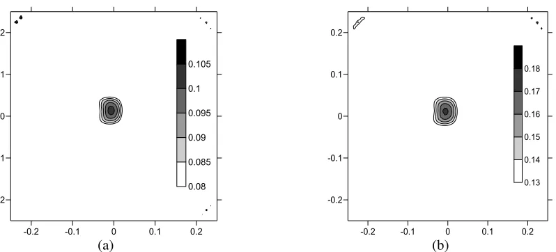
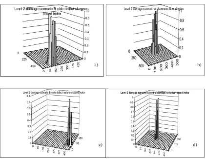
Now the use of the two statistics based on the distribution of points on the attractor, the indexes Fs and Fσ will be demonstrated. If there is no change in the damage state these indexes should be close to 0 while if there is a change in the damage state of the plate these indexes are expected to increase. In this numerical example it was assumed that measurements are taken in a net of 16 equally distributed points that cover the surface of the plate. The global indexes were calculated using the signals obtained in all the 16 points, while the local indexes were calculated for the signals obtained in each one point. The global indexes can be used preliminary for dam-age detection. For the purposes of detection and localization the local indexes should be preferred. Figure 7 details the local skewness-based and variance-based indexes (9) for central and side defect for the second dam-age level. It should be noted that both indexes are capable to localise the damdam-age. It can be appreciated that the variance-based index gives a sharper and more precise localisation of the damage while with the skewness-based index the localization is a bit smeared.

-0.1 0.0 0.1

displacements, m

-160 -120 -80 -40 0 40

ve

lo

ci

ty

, m

/s

-0.04 0.00 0.04

displacements , m 0

50 100

ve

lo

ci

ty

m

(a) (b)

Figure 5. Contour map of damage index FPfor central damage (Case A), a) level 1; b) –level 2.

(a) (b)

Figure 6. Contour plots side damage (a) -level 1,(b)- level 2

-0.2 -0.1 0 0.1 0.2

-0.2 -0.1 0 0.1 0.2

0.08 0.085 0.09 0.095 0.1 0.105

-0.2 -0.1 0 0.1 0.2

-0.2 -0.1 0 0.1 0.2

0.13 0.14 0.15 0.16 0.17 0.18

-0.25 -0.15 -0.05 0.05 0.15 0.25

-0.25 -0.15 -0.05 0.05 0.15 0.25

Figure 7: The skewness-based a), b) and the variance-based c),d) indexes for side defect a),c), and cen-tral defect b),d)

3.5. Case study 2 .Structural Damage Detection in a Reinforced Concrete Slab

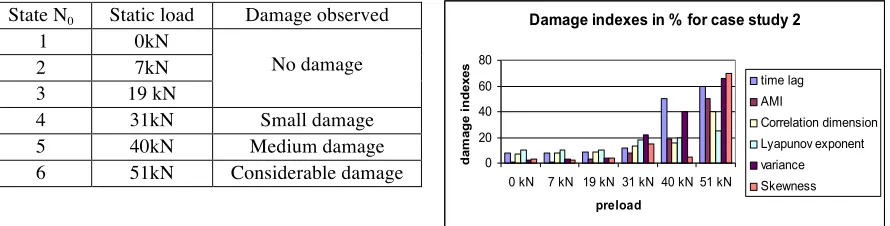
In this study a reinforced concrete slab with the following dimensions 1420mm x 1420mm in plan and 75 mm in depth is tested. The experiment was performed in cycles. At each loading cycle a static load is slowly ap-plied at mid-span. Then the static load is removed and the slab is dynamically excited and its acceleration re-sponse is measured in the position indicated. A random excitation signal is used for the dynamic experiment and the reason for this is that in most practical situations structures are subjected to ambient excitation. Then a new increased static load is applied and the dynamic response of the slab is measured in its new state achieved after the removal of the load. The static load spanned from unloaded state to the ultimate state of failure. The damage levels introduced are given in Table 1 below.

a)

c)

0

225

450

0 75 150 225 300 375 450

0 0.1 0.2 0.3 0.4 0.5 0.6 0.7

Level 2 damage scenario B side defect skewnes-based index

0 250

500

0

100 200 300 400 500

0 0.2 0.4 0.6 0.8 1

Level 2 damage scenario A skewness-based index

0

75

150 ₂₂₅ 300 ₃₇₅

450

0 175

350 0

0.1 0.2 0.3 0.4 0.5 0.6 0.7 0.8

Level 2 damage scenario B side defect variance-based index

0

75

150 ₂₂₅ 300 ₃₇₅

450

0 175

350 0

0.1 0.2 0.3 0.4 0.5 0.6 0.7 0.8 0.9 1

Level 2 damage scenario A central damage variance- based index

a) b)

Figure 8 gives the changes in the above introduced indexes with damage. It includes the indexes based on time delay FT, the mutual information FI, the correlation dimension FD and the Lyapunov exponent Fλas well as the

indexes based on the statistical characteristics of the distribution Fσ and Fs. The ones for the time lag, the

Lya-punov exponent and the correlation dimension are quite high for the first three levels of preload which actually correspond to no-damage level. They change just a little bit for the first level, 31kN preload and for the next level the time lag-based index jumps to 50 and it still increases for the last level corresponding to large damage. Thus it will be possible to detect and recognize the medium and the large damage but not the small level dam-age. The other indexes based on the invariants, vis the ones based on the Lypunov exponent and the correlation dimension remain very much unchanged- they increase a little bit for the for the 1st damage level and then stay very much on the same level. So these indexes in this case will not be very helpful neither for detecting nor for estimating the damage level All the invariant-based indexes will give a false alarm for the case of no damage if e.g. threshold of 5% is selected. Thus a higher threshold is needed for these indexes but then the small level damage might be unrecognized. The other two indexes, the ones based on the variance and the skewness, be-have more or less as expected: they are below 5% for the no-damage cases and they gradually increase for the subsequent levels which means they can be used to detect even the smallest level of damage and also to distin-guish between the different damage levels. Thus these two indexes are much more useful and easy to estimate from data as compared to the indexes based on the attractor invariants.

3.6. Case study 3. Backlash Detection in Robot Joints

The phase space approach can be applied and has been applied for the purposes of machinery analysis and monitoring. The phase space methodology has been suggested and applied for the purposes of machinery moni-toring by several authors (Matthew 1997, Trendafilova&Van Brussel 2001, Trendafilova et al 1999,2000). In this study the approach is demonstrated for the analysis and the detection of backlash robot joints.

The dynamics of a robot joint is commonly rather complex. Some phenomena to be taken into account are friction, deformation of non-linear materials, geometry of the part, dynamics and geometry of the other parts connected to the joint. In general, robot joints demonstrate non-linear dynamic behaviour, which can be due to a number of different reasons and is caused by different mechanisms. The presence of non-linearities and the consequent non-linear behaviour exhibited by robot parts is a problem that gives rise to serious difficulties in the kinematic and especially the dynamic modelling, analysis and control of robot joints. It becomes rather difficult to develop an accurate model that takes into account the different phenomena (like friction, joint and link flexibility, backlash and clearances) that influence the system dynamics. The non-linear behaviour poses serious difficulties in the process of the analysis of signals recorded from different elements and in the related inverse dynamic problems, i.e. identification and control which are rather important for the design and analysis of robotic structures and their components.

In this study, the data-dependent approach is used to analyse the behaviour of robot joints, for several cases when a backlash is present including the case of no backlash, from the standpoint of non-linear dynamics,

mak-State N0 Static load Damage observed

1 0kN

No damage

2 7kN

3 19 kN

4 31kN Small damage

5 40kN Medium damage

6 51kN Considerable damage

Damage indexes in % for case study 2

0 20 40 60 80

0 kN 7 kN 19 kN 31 kN 40 kN 51 kN

preload

da

m

a

ge

i

nde

x

e

s

time lag AMI

Correlation dimension Lyapunov exponent variance Skewness

Table 1: Static pre-loads and corresponding slab states

ing use of the recorded acceleration signals. The approach is based on the assumption that a backlash introduc-es a linearity in the joint. Thus, in all casintroduc-es when backlash is printroduc-esent in the joint we are dealing with non-linear motion. Accordingly, the non-non-linear motion invariants are supposed to change with the change of the backlash size. Then the non-linear invariants might be employed to generate features from the recorded signals and use them for backlash detection and quantification. All these assumptions were proved by using the time data from the response acceleration signals in (Trendafilova& VanBrussel 2001,Trendafilova et al. 2000). We first analyze the behaviour of robot connections when different backlash is present and in the state of no back-lash starting from their time responses, spectra and using pseudo-phase-space representations. The next step is to recover the embedding space necessary to unfold the motion for all the types of joints considered. This in-cludes the determination of the time lag and the embedding dimension. We further try to establish the kind of dynamic behaviour for all the categories of joints we introduce using surrogate data tests. It is demonstrated that for the robot joints despite the periodic behaviour of the arm, there is another component which makes the motion definitely non-linear, especially when looking at a single transient (Trendafilova&Van Brussel 2001). We prove that this component is a non-linear deterministic one. Thus a non-linear deterministic model for the dynamic behaviour of robot joints can be recovered. Unfolding their dynamics and recovering the embedding time delay space is the first step towards reconstructing a model. By using the recovered embedding state space, we are now able to more accurately estimate some of the motion invariants for all the joint types. The consequent determination of some non-linear (chaotic) dynamics invariants (Lyapunov exponents, attractor dimensions) confirms some conclusions, already suggested from the previous analysis. The obtained Lyapunov exponents suggest the degree of chaos for the considered signals. They prove the conclusions, already implied by the surrogate data tests: there is weak chaos in the cases of no backlash and small backlash and the degree of chaos increases with the increase of the backlash size. Ultimately, the reconstruction of the unfolding space can be used for building local and global models of the dynamics of the system. Such kinds of models can be uti-lized to develop procedures for defect qualification and quantification, applying inverse identification methods.

3.6.1. Experiments with Industrial Robots.

Experiments were conducted on a PUMA 762 industrial robot. The aim is to analyse the time response of some robot joints in the presence of a backlash and in normal condition (no backlash). For this purpose, various de-grees of backlash were introduced in two joints of the robot by adjusting the backlash screws of the robot links. The joints are rotational and each of them is driven by a servomotor and gear transmission. The dynamic re-sponses are measured with an accelerometer mounted on the end transmission. Two series of experiments were

performed with backlash in each joint with the following backlash sizes, vis. zero (i.e. no backlash), small,

medium and maximum backlash.

3.6.2. Signal Analysis.

In accordance with the experiments performed, and in correspondence with the joint type from which the sig-nals come, we introduce four signal categories: no backlash sigsig-nals (N), small backlash sigsig-nals (S), medium backlash signals (M) and large backlash signals (L). At first glance, the vibration signatures coming from the robot joints look very much periodic, since the joints rotate with constant frequency. But we were able to estab-lish that there is another component besides the periodic one (Trendafilova&Van Brussel 2001). In order to observe it the signals were high-pass filtered. Since the visual appearance of the signals does not suggest any features to distinguish between signals coming from a damaged and a non-damaged link and since all the signal spectra were broadband which made them difficult to analyze and extract any features from we used a pseudo-phase-space representation (Abarbanel 1996). The presumption is that the plot will mimic the behavior of the real system and the pseudo-phase-plane technique is expected to preserve the major properties of the system,

and thus to enable us to draw some conclusions for the motion. From the analysis of the signals as well as from

the backlash becomes. This has been proved in two previous studies (Trendafilova et al 1999,Trendafilova&Van Brussel 2001) by using hypothesis analysis. The next section considers the process of backlash detection and quantification.

3.6.3. Detecting Backlash Using the Phase Space Representation

We were able to establish that there are several phase space invariants that change as a result of the introduc-tion and the growth of backlash. Two of these characteristics, the Lyapunov exponent and the correlaintroduc-tion di-mension of the phase space were used in order to detect and quantify backlash in robot joints. A pattern recog-nition method was used and the following categories were introduced:

-the category of signals from a no backlash joint N,

-the category of signals from a joint with a small backlash S, -the category of signals from a joint with a medium backlash M and -the category of signals from a joint with a large backlash L.

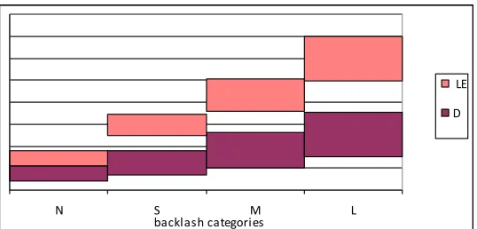
It is our aim to distinguish among these categories, extracting information directly from the measured vibration signals and making use of the recovered embedding dimension to estimate the characteristics of the corre-sponding time series. This can be achieved by using the above results, namely exploiting some non-linear dy-namics characteristics of the signals. We were able to establish that the maximum LEs vary for the different categories. They have the smallest values for the case of N signals increasing with the introduction and the growth of backlash. Consequently, the maximum Lyapunov exponents can be used as features to distinguish among the introduced categories. Another characteristic that was be observed to differ for the different catego-ries is the correlation dimension. It is a geometric characteristic of the motion and gives an idea about the di-mension of the attractor. It is also expected to increase with the increase of the degree of chaos. Our results suggest the same tendency as for the LE: the smallest correlation dimensions are registered for the N category and they increase with the increase of the backlash extent. Accordingly, one can try to use the correlation di-mension also as a feature. Figure 9 shows the ranges for the Lyapunov exponents and the correlation didi-mension for the different categories. Thus, a very natural way to try to distinguish among the considered categories is to develop a classifier using as features the maximum Lyapunov exponent and the correlation dimension. Instead of the signals their Lyapunov exponents λj and the correlation dimension D are used, thus forming a pattern

vectors for each signal. A rather simple classifier is the one which utilises the nearest neighbour (NN) rule and the Euclidean distance as a dissimilarity measure. In order to build such a classifier, we take a prototype sample with known categorisation, i.e. each of the pattern vectors belongs to one of the considered categories. The NN classifier categorises a test signal to the category to which its nearest neighbour belongs. Thus e.g. a signal is considered to belong to the class N (no backlash) if its nearest neighbour belongs to this category.

Figure 9: Ranges for the correlation dimension D and the Lyapunov exponent LE

N S M L

backlash  categories

 LE

For this study, 139 signals (35 of them from the N category, 33 from S, 36 from M and 35 from L) were meas-ured from the PUMA robot axes to form the prototype sample of feature vectors with known categorisation. Then, the performance of the developed classifier was checked with another test sample of signals 96 signals from the PUMA robot axes. Table 2summarises the results for the performance of the classifiers. The numbers on the main diagonal give the percentage of correctly classified signals for the quantification classifiers and the detection classifiers, respectively. The figures outside the diagonal give the percentage of the incorrectly classi-fied signals. In general it can be seen that the classifier demonstrate rather good performance in distinguishing among the different signal categories.

5.

Influence of Temperature and Environmental Conditions on the Nonlinear

Vi-bratory Behaviour of Structures

All approaches in health monitoring systems are based on the argument that damage in the structure will cause changes in the measured vibration data. Many existing methods, however, neglect the important effect of changing the environment of the underlying structure. For structures in operational conditions, the variability in dynamic properties and dynamic behavior can be a result of time-varying environmental conditions. Environ-mental conditions include, temperature, humidity and eventually wind (if the structure is exposed to wind).

Certainly, the temperature variation is the most important factor which can influence the health monitoring procedure. It not only changes the material stiffness, but also alters the boundary conditions of a system. (Sohn,2007). The temporal variation of the temperature also needs to be noted. Many structures exhibit daily and seasonal temperature variations. Thermal loads introduce stresses due to thermal expansion, which lead to changes in the modal properties. Thermal loads can also cause buckling and in some cases even lead to chaotic behaviour (Amabili et al. 2009, Manoach et al. 2004, Ribeiro et al. 2005 ,2007). Thus, on a lot of occasions the presence of a temperature field can either mask the effect of damage or increase it, which will render a VSHM method ineffective - it might give no alarm when a fault is present or give a false alarm. This is why it is vital to be able to take into account the temperature changes when developing VSHM procedures.

Few authors have investigated the long-term stability against humidity variation (Manson et al. 2001). The authors report that while temperature variation mainly produced a phase shift of the signal with a slight ampli-tude change, humidity changed the ampliampli-tude of the Lamb-wave response. However, the authors concluded that Lamb-wave propagation characteristics were more sensitive to temperature variations than changes in humidi-ty.

As far as it is practically impossible to distinguish the influence of mechanically induced changes in the re-sponse of the structures from the thermally induced ones (Pirner & Fischer 1997) we shall use the damage in-dex and the corresponding criterion defined in & 3.1 with equations (4) and (5).

Thus, if the following criterion is fulfilled

F

(

X

,

Δ

T

)

>

T

one can conclude that the beam is damaged and the sets of points (X) for which Eq.(14) is fulfilled, form the damaged area (areas). The essential point here is that the temperature changes should also be taken into

ac-N S M L

True class N 92 7 1 0

True class S 7 91 2 0

True class M 0 1 93 6

True class L 0 0 5 95

count. For this reason the damage indexes defined by Eqs. (4) and (5) should be calculated at equal values of ΔT for the healthy and damaged beams.

To show the influence of the temperature on damage assessment and localization of structures two numeri-cal examples are shown – for a beam and for a plate. The beam has length l=80 mm thickness h=2.5 mm and the width b=5 mm. The characteristics of the beam’s material are Young’s modulus E=41.92 GPa, Poisson’s ratio ν=0.32991, density ρ=2052 kg/m3andthe coefficient of thermal expansionαT=13.2×10-6 K-1.The material

properties correspond to the effective properties of laminated composite. For the considered beam geometry damage (delamination) is located atx∈(0.56m, 0.64m) (10 % of the beam length). It is modelled by prescribing

to this part of the beam reduced rigidity Ed = 0.5E = 20.96 GPa. The beam is discretized by 40 linear beam finite elements.

The second numerical example concerns a thick aluminium rectangular plate with the following geomet-rical and material properties: a = 10 m, b = 2.5 m, h = 0.05 m, Young’s modulus E = 7.1010 N/m2, Poison ratio

ν= 0.34, density ρ= 2778 kg/m3. The finite element discretization and the damage area are shown in Fig. 16. In this case the damaged area is modelled as an area with reduced thickness hdamaged = h/2, (h is the thickness of

the plate). The plate is fully clamped and the applied harmonic load p = 500 N is uniformly distributed over the whole plate surface.

First of all, the sensitivity of the first 7 natural frequencies of the beams and plates (calculated by finite el-ement method) to damage was tested. The results show that the considered defects cause very small changes (less than 5% )in the natural frequencies of the beam. The changes in the eigen frequencies of the plate due to damage are even smaller. Obviously such small changes cannot be used as an indicator for damage.

Then the forced response of the beam subjected to a harmonic loading is tested. The beams are subjected to two kinds of loadings: (a) excitation with frequency equal (or very close) to the first natural frequency and (b) excitation with frequency equal to a half of the first natural frequency. The beams are additionally subjected to different temperature loads: ΔT=10 K, ΔT=20 K and ΔT=30 K. In all cases time history diagrams and Poin-caré maps are plotted for intact (healthy) and damaged beams.

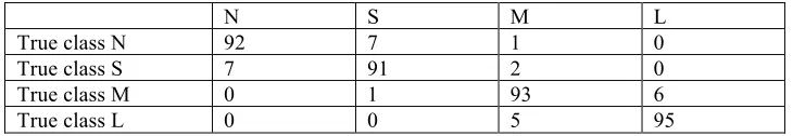
Let us first have a look at the time histories of the beam’s responses. In the cases when the excitation fre-quency is close to the first natural frefre-quency of the beam a beating phenomenon is observed (Manoach et al., 2004, 2008). The influence of damage on the time history diagrams of the beam subjected to a loading with excitation frequency ωe= 5665 rad/s (~ω1/2) at different temperature changes can be seen in Figs 10 a,b. In

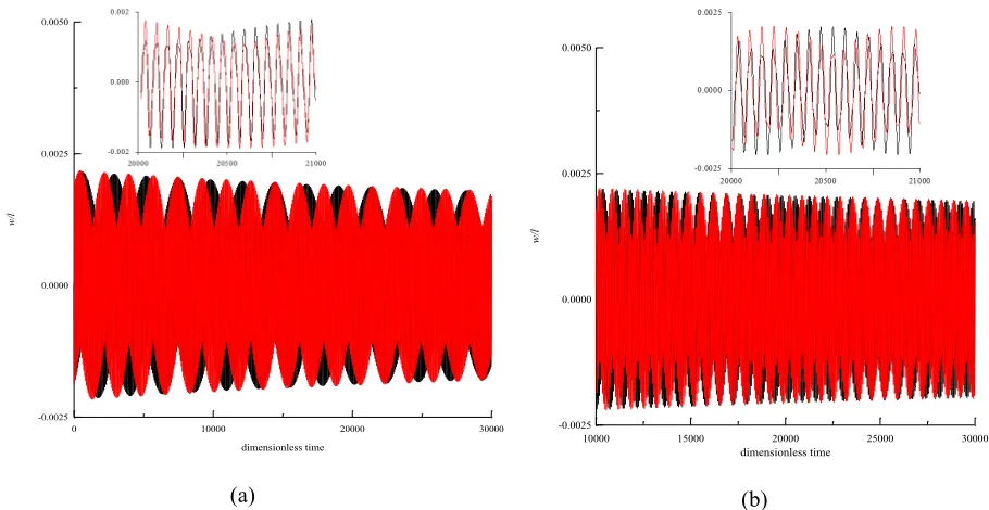
Figs 11 a,b the time history diagrams at excitation frequency almost equals to the first natural frequency of the healthy beam (ωe= 11330 rad/s) are shown. From these time-history diagrams it can be concluded that the

considered damage leads to small changes in the amplitude of responses but the time histories undergo signifi-cant changes in the period of beating . It can be seen that at the very beginning (t=0) the responses almost coin-cide. Then the phase shifts and the differences between the responses increase (see small figures inserted in the main figures where the time history are shown for a very short period of time).

The changes are more essential when ωe = ω1. It is reasonable to expect that small changes in the first

natu-ral frequency due to damage are more important when a beam is excited in the most sensitive frequency region. The computations confirm these expectations. Figures 12 a,b and 13 a,b show that the considered damage does not change the type of the Poincaré map but it only slightly influences the size of the radius of the circle formed by the dots. Nevertheless, in all cases of temperature loading the presence of damage and its location is very well predicted by the damage criterion based on the damage index (see Figs 14 and 15). It is important to notice that when

_ω

ele-vated temperature strengthens the influence of damage. However, when

_ω

one tries to construct a damage index by using data for the unheated healthy beam and for the heated damaged beam the damage location cannot be predicted as can be seen in Fig. 16.

A similar study was performed in the case of the above described plate. The time history diagrams of the plate centre with defect and without defect are shown in Fig. 18. The same time history diagrams but in the case of elevated temperatures of the plates are shown in Fig. 19. The excitation frequency is 260 rad/s, which is 7 % less than the first eigen frequency of the healthy plate.

(a) _(b)

Figure 10: Time histories of the beam centre for different temperatures. p=50 N, ωe= 5665

rad/s,. (a) - ΔT=10; (b) ΔT=30 Black line – healthy beam; red line –damaged beam

A strong beating can be observed in the responses of the healthy and damaged plates. The phase of the re-sponse of the damaged plate shifts and the difference between the rere-sponses increases with the time. The same conclusion applies in the case of the rectangular plate at elevated temperature. The elevated temperature leads to larger values of the vibration amplitude. Again, the differences between the Poincaré plots of the heated and unheated plates are largest for the points from the damaged areas (see Fig. 20 a-c). Accordingly, the damage indexes corresponding to the damaged area have the biggest values, which gives the possibility to locate the damage. The contour plots of F_iP corresponding to three different temperatures are shown in Fig. 21. It can be seen that the damage location is predicted very precisely in the case of the unheated plate as well as in the cases of the heated plate with two different temperatures ΔT = 50 K and ΔT = 100 K. The threshold value Td

is set to 0.28 for all cases and the maximal value of Id is almost the same (Id = 0.4 for ΔT = 0, ΔT = 50 K and

Id = 0.42 for ΔT = 100 K).

0 10000 20000 30000 dimensionless time

-0.0025 0.0000 0.0025 0.0050

w

/l

10000 15000 20000 25000 30000 dimensionless time

-0.0025 0.0000 0.0025 0.0050

w

(a) _(b)

Figure 11: Time history diagrams of the beam centre at different temperatures.(a) - ΔT=10, (b) -_ΔT=30 p=50 N, ωe= 11330 rad/s, Black line – healthy beam; red line –damaged beam

(a) _(b)

Figure 12: Poincaré maps for the response of the beam centre at different temperatures p=50 N, ωe= 5665 rad/s.. (a) - ΔT=10, (b) -ΔT=30 .Black dots – undamaged beam, red

dots – damaged beam

0 10000 20000 30000

dimensionless time

-0.025 0.000 0.025 0.050

w

/l

0 10000 20000 30000

dimensionless time -0.03

0.00 0.03 0.06

w

/l

-0.002 0.000 0.002

w/l

-0.0002 0.0000 0.0002

di

m

en

si

on

le

ss

v

el

oc

it

y

-0.002 0.000 0.002

w/l

-0.00025 0.00000 0.00025

di

m

en

si

on

le

ss

v

el

oc

it

(a) (b)

Figure13: Poincaré maps for the response of the beam centre at different temperatures p=50N, ωe=

11330 rad/s. (a) ΔT=10, (b) -ΔT=30 .Black dots – undamaged beam, red dots – damaged beam

ΔΤ=0

ΔΤ=20

ΔΤ=30

ΔΤ=10

1 11 21 31 41

Node numbers 0.000

0.003

D

am

ag

e

in

de

x

Damaged area

Figure 14: Damage index for a beam subjected to har-monic mechanical loading with an amplitude p=50 N, excitation frequency ωe= 5665 rad/s and different

thermal loads

1 11 21 31 41

Node number 0.00

0.08 0.16

D

am

ag

e

in

d

ex

ΔΤ=0

ΔΤ=10

ΔΤ=20

ΔΤ=30

Damaged area

Figure 15: Damage index for a beam subjected to harmonic mechanical loading with an amplitude

p=50 N, excitation frequency ωe= 11330 rad/s and

different thermal loads

-0.02 0.00 0.02

w/l

-0.004 0.000 0.004

di

m

en

si

on

le

ss

v

el

oc

ity

-0.03 0.00 0.03

w/l

-0.005 0.000 0.005

di

m

en

si

on

le

ss

v

el

oc

Figure 16: Damage index computed when the healthy beam is at ΔT=0 and the damaged beam is at ΔT=20 K

Figure 17: Finite element mesh of the plate with defect

Figure 18: Time history diagram of the plate centre, p

= 500N, _ωe= 260 rad/s

Figure 19: Time history diagram of the plate centre of heated plate , p = 500N, _ωe = 260 rad/s, ΔT = 50 K

5.

Discussion. Concluding remarks

The aim of this chapter is to introduce some new applications of nonlinear dynamics tools and nonlinear signal analysis for VHM of structures and machinery (robotic mechanisms in particular). The main contributions of this study are in the introduction and the development of several novel procedures based on nonlinear dynamics

1 11 21 31 41

Node number 0.000

0.015

D

am

ge

in

de

x

0 2 4

time, s -0.12

-0.06 0.00 0.06 0.12 0.18

di

sp

la

ce

m

en

ts

, m

0 _{time, s} 5

-0.15 0.00 0.15

d

is

p

la

ce

m

e

n

ts

,