Bhowmik, S. K. and Duncan, D. B. and Grinfeld, M. and Lord, G. J. (2011)
Finite to infinite steady state solutions, bifurcations of an
integro-differential equation. Discrete and Continuous Dynamical Systems -
Series B, 16 (1). pp. 57-71. ISSN 1531-3492 ,
http://dx.doi.org/10.3934/dcdsb.2011.16.57
This version is available at https://strathprints.strath.ac.uk/35064/
Strathprints is designed to allow users to access the research output of the University of Strathclyde. Unless otherwise explicitly stated on the manuscript, Copyright © and Moral Rights for the papers on this site are retained by the individual authors and/or other copyright owners. Please check the manuscript for details of any other licences that may have been applied. You may not engage in further distribution of the material for any profitmaking activities or any commercial gain. You may freely distribute both the url (https://strathprints.strath.ac.uk/) and the content of this paper for research or private study, educational, or not-for-profit purposes without prior permission or charge.
Any correspondence concerning this service should be sent to the Strathprints administrator: [email protected]
The Strathprints institutional repository (https://strathprints.strath.ac.uk) is a digital archive of University of Strathclyde research outputs. It has been developed to disseminate open access research outputs, expose data about those outputs, and enable the
arXiv:1004.5136v1 [math.DS] 28 Apr 2010
Finite to infinite steady state solutions, bifurcations of an
integro-differential equation
S. K. Bhowmik1, D. B. Duncan2, M. Grinfeld3, G. J. Lord4
April 30, 2010
1
KdV Institute for Mathematics, University of Amsterdam, Amsterdam, NL, [email protected].
2
Department of Mathematics and Maxwell Institute, Heriot–Watt University,Edinburgh, UK, [email protected]
3
Department of Mathematics, University of Strathclyde, Glasgow, UK, [email protected]
4
Department of Mathematics and Maxwell Institute, Heriot–Watt University,Edinburgh, UK, [email protected]
Abstract
We consider a bistable integral equation which governs the stationary solutions of a convolution model of solid–solid phase transitions on a circle. We study the bifurcations of the set of the stationary solutions as the diffusion coefficient is varied to examine the transition from an infinite number of steady states to three for the continuum limit of the semi–discretised system. We show how the symmetry of the problem is responsible for the generation and stabilisation of equilibria and comment on the puzzling connection between continuity and stability that exists in this problem.
1
Introduction
Integro-differential equations are used to model various phenomena in materials science [1, 2, 3, 5, 9, 17] and biology [7, 8, 21, 25], which involve non-local diffusion/dispersal mechanisms. We consider the integro-differential equation (IDE)
ut=ε Z
R
J∞
(x−y)u(y, t)dy−u(x, t)
Z
R
J∞
(x−y)dy
+f(u), (1)
where the L1(R) kernel J∞ satisfies J∞(x) ≥ 0, J∞(x) = J∞(−x) and f(u) is a bistable
nonlinearity. Below we routinely consider f(u) =u(1−u2) and kernel
J∞
(x) =
r
100
π exp(−100x
2), (2)
so that R
RJ
∞
dx = 1. To obtain a well-defined problem, (1) has to be supplemented by a suitable initial condition, u(x,0) = u0(x) which needs to be chosen in a suitable function
space, see [15, 19, 16].
The convolution equation (1) is theL2-gradient flow of the free energy functional
E(u) = 1 4ε
Z
R Z
R
J∞
(x−y) (u(y)−u(x))2dxdy+
Z
R
ˆ
F(u)dx, (3)
For an overview of the use of (1) in materials science, see [10]. There are many papers dealing with the mathematical analysis of this equation, which examine existence and stability of trav-elling waves [3], the structure of the stationary solutions set [2], propagation of discontinuities [11], coarsening [9] and long time behaviour [15, 19, 24, 20].
Note, in particular, that in [15] it is shown that if the diffusion coefficient ε is sufficiently large, a “Conway–Hopf–Smoller” type result holds: the only stable steady state solutions, say, in L∞(
R), are the constant stable steady states of the kinetic equation ut=f(u). Thus, if we choose f(u) = u(1−u2), the stable states are u= 1 and u=−1. On the other hand, if ε = 0, (1) admits an uncountable set of equilibria: let X, Y and Z be any disjoint sets such that A∪B ∪C = R, then a function u(x) that is equal to 1 on X, −1 on Y and 0 on Z is a steady state solution. Note that if Z = ∅, all the resulting equilibria are stable inL∞(I). Furthermore, it is shown in [9] that there exists an ε
0 >0 which depends on the
kernelJ∞, such that for all 0< ε < ε
0 the set of steady state solutions of (1) is in one-to-one
correspondence with the set of equilibria ofut =f(u). Hence, in view of the above, it is of interest to perform a bifurcation analysis of the set of steady states of (1),
0 =ε
Z
R
J∞
(x−y)(u(y)−u(x))dy+f(u), (4)
as we decreaseεfrom some initially large value to zero, and investigate the transition from a finite to infinite set of solutions.
To the best of our knowledge, such a study has not been performed before. The object of this paper is precisely such a study of the spatially discretised version of (1). For simplicity, here we restrict ourselves to 1-periodic patterns.
If we choose spatially one-periodic initial data u(x,0), then from (1) it is clear that for all
x∈Rand t∈R+
u(x, t) =u(x+ 1, t).
Then from (1) we have
ut=ε Z
R
J∞
(x−y) (u(y, t)−u(x, t))dy+f(u)
=ε
∞
X
r=−∞
Z r+1
r
J∞
(x−y) (u(y, t)−u(x, t))dy+f(u)
=ε
∞
X
r=−∞
Z 1
0 J∞
(x−z−r) (u(z+r, t)−u(x, t))dz+f(u)
=ε
Z 1
0
J(x−z) (u(z, t)−u(x, t))dz+f(u), (5)
where
J(x) =
∞
X
r=−∞
J∞
(x−r) (6)
and x∈[0,1]. Thus, for 1-periodic initial data we only need to solve the problem (1) on the interval Ω = [0,1] with the kernel J(x). For the kernel given by (2), J∞
Lemma 1. For J defined by (6) the following two properties hold. 1. IfJ∞
(x) =J∞
(−x) we have that
J(x) =J(1−x).
2. R1
0 J(x)dx=
R∞
−∞J
∞(x)dx.
Property 1. above has an important influence on the spectrum of the matrix governing the semi-discretised version of (1) as we explain in the next section. From now on we work on [0,1] and use the kernel J given in (6)
(a) (b)
−1 0 1
0 1 2 3 4 5
x
0 0.5 1
0 1 2 3 4 5
[image:4.612.104.496.246.403.2]x
Figure 1: The kernels J∞(x) in (a) andJ(x) in (b) for the case of equation (2).
2
The semi-discretised system
We discretise in space using piecewise-constant functions [9] and collocating at the uniformly spaced element mid-points,x=xj+1
2,j= 0,1,2,· · · , N−1. Settinguj =u(xj+ 1
2, t), we have
the semi-discrete approximation of (1) given by
ut=εANu+F(u), (7)
where now u(t) ∈ RN, supplemented with some initial condition u(0) = u0 ∈ RN. The
nonlinearityF :RN 7→RN is given byFj(u) =f(uj). It remains to specify theN×N matrix
AN. If we puth= N1, its elements are given by
aj,i= (
hJ(|xj−i|) j6=i
hhJ(0)−PN
r=1 J(|xj−r|) i
j =i. (8)
From Lemma 1 it follows thatAN is a symmetric circulant matrix generated by the elements
Proposition 1 ([23]). Let AN be the circulant matrix defined by a1,1, a1,2, ..., a1,N. Then
−AN is diagonalisable with eigenvalues
λk=−[a1,1+a1,2Wk+a1,3Wk2+...+a1,NWkN−1], (9)
with corresponding eigenvectorsvk=
1, Wk, Wk2, ..., WN
−1
k
T
.
Let us see what this implies in our case for the spectrum of the discretisation.
Lemma 2. The following three properties hold for the spectrum of AN
1. λ0 = 0; 2. λk=λN−k;
3. Let IN be the convex hull of the set of non-zero eigenvalues of AN. As N → ∞, IN
converges in the Hausdorff metric to the set
I∞=
Z 1
0
J(x)dx−
Z 1
0
J(x) exp(2πix)dx,
Z 1
0
J(x)dx.
.
Before we prove this lemma, let us explain what it means. First of all, we must have a zero eigenvalue with a constant eigenvector, because, like in the case of the Neumann Laplacian, the equation
ut=
Z ∞
−∞
J∞
(x−y)(u(y, t)−u(x, t)) dx,
conserves mass.
Secondly, the pairing of the eigenvalues is simply the consequence of the symmetry J(x) =
J(1−x) inherited from the evenness of the kernel J∞. Finally, the third part of the lemma
implies that asN → ∞, the spectrum accumulates at the pointR1
0 J(x)dx. Note that in the
case ofJ∞(x) = p
100/π exp(−100x2), we explicitly have
I∞= [1−exp(−π2/100),1] = [0.094,1].
Proof. 1. From (8), puttingW0 = 1, we immediately obtain from (9) thatλ0= 0.
2. From part 1. of Lemma 1 it follows that for allj= 2, . . . , N,
a1,j =a1,N+2−j,
so that the matrix AN is symmetric. Hence its eigenvalues λk are real. But then taking complex conjugates ofANvk=λkvk, we get thatANvk=λkvk, or in other wordsAnvN−k=
λkvN−k and henceλk=λN−k.
3. Finally, by taking the limit asN → ∞ in (9) we immediately obtain that
λk →
Z 1
0
J(x)dx−
Z 1
0
J(x) exp(2πikx)dx,
k= 1,2, . . ..
from the trivial solutionu= 0. Here we examine analytically the values of εwhere such bi-furcations may occur in the semi-discrete system and later we can compare to the numerically found values. Linearising around the zero solution, we have the eigenvalue problem
εANv+ gradF(0)v=µv, (10)
and hence bifurcations from the zero solution will only occur ifµ= 0, or in other words, if
−ANv=
f′(0)
ε v.
Thus, for the semi-discrete system (7) we can fully characterize the values ofε where bifur-cations of the zero solution occur, namely
εk:=
f′(0)
λk
, k= 0, . . . , N−1. (11)
For example, for N = 32,J∞
(x) =
q
100
π exp(−100x2) and f(u) = u(1−u2), we have using (9), the results of Lemma 2 and the formula (11) that bifurcations from the zero solution are expected at the values of εas in Table 2. Note that for this case of N = 32, the value ofε1
agrees to 12 decimal points with the limiting value of ε1, 1/(1−exp(−π2/100)) as N → ∞,
(see part 3 of Lemma 2).
ε1 =ε31 10.6403416996149 ε9 =ε23 1.00033746722800 ε2 =ε30 3.06584313146254 ε10=ε22 1.00005172586163 ε3 =ε29 1.69885748860222 ε11=ε21 1.00000650971543 ε4 =ε28 1.25968856776757 ε12=ε20 1.00000067252291 ε5 =ε27 1.09266327932320 ε13=ε19 1.00000005703325 ε6 =ε26 1.02948119722480 ε14=ε18 1.00000000397031 ε7 =ε25 1.00800141737791 ε15=ε17 1.00000000022729 ε8 =ε24 1.00180943793728 ε16 1.00000000002128
Table 1: ForN = 32 Bifurcation values in terms of εof the zero solution.
Let us examine the eigenvectors of −AN in some more detail. Since bothvk and vN−k are eigenvectors, we immediately have that Re (vk) and Im (vk) are eigenvectors. Define the cyclic shiftσ on u= (u1, . . . , uN)∈RN by
σ(u) = (uN, u1, . . . , uN−1),
then we have
Lemma 3. If v is a real eigenvector of−AN corresponding to a double eigenvalue λ, then so
isσ(v).
This follows since ifv is an eigenvector, then so ise2iπ/Nv.
Remark. In the above argument, we can pass to the limit as N → ∞ and arrive at the somewhat startling conclusion that cos(2πkx) and all their translates are eigenfunctions of
−A = −(R1
the right symmetry property. Of course, cosines are also the eigenfunctions of the Neumann Laplacian. It is very pleasing to obtain such a result via a semi-discretisation.
Finally we note that fixed points of the semi-discrete problem satisfy
0 =εANu+F(u). (12)
Thus at ε= 0 stable solutions are given by
u=
1 x∈X,
−1 x∈Y (13)
where X∪Y = [0,1]. Unstable solutions atε= 0 are given by
u=
1 x∈X, −1 x∈Y ,
0 x∈Z
(14)
where X∪Y ∪Z = [0,1] with some nonemptyZ.
We use this to define solutions with different numbers of interfaces. When X = [0, α) and
Y = [α,1], 0 < α < 1, we call u a one-interface solution of (12) if for ε = 0 for some
n∈ [0, N −1], σn(u) = a1 on X = [0, α) and σn(u) = a2 on Y = [α,1], a1a2 ∈ {−1,0,1}, a1 6= a2. That is loosely speaking we have at ε = 0 one jump in the solution upto cyclic
shift. Two-interface, three-interface solutions, etc., are defined similarly. Thus, for example, the branch of solutions corresponding to orbit A in Table 2 are of one-interface and those corresponding toE are of three-interface.
3
Results
We take for our computations the kernel function
J∞
(x) =
r
100
π e
−100x2
,
with f(u) = u(1−u2) and vary the parameter ε. For small values of N it is possible to
enumerate all possible solutions of the semi-discrete system (12) with ε = 0 and to analyse their continuation toε >0 using the theory of bifurcation with symmetry. This we do below forN = 4 and these analytic results were used to check the validity of our numerics.
We implemented inMatlaba standard pseudo arc–length continuation algorithm with step size control as described in [14, 22, 13] for the discrete problem (12). SinceAN is a circulant matrix, we take advantage of reducing storage costs as the full information of AN can be obtained storing one row or column only, see [4] and references therein. Furthermore the use of the FFT for each matrix vector multiplication reduces the computational cost. We detect bifurcation points by observing where eigenvalues of the Jacobian J =DuF of the nonlinear system F(u, β) = 0 cross the imaginary axis and perform branch switching at those points by perturbing in the direction of the associated eigenvector.
The arc-lengthℓ ofu(x)∈C1(R) is defined in the standard way
ℓ=
Z
Ω
s
1 +
du dx
2
and we approximate the arc–length ofu(x) with the mid-point rule and using the standard forward difference approximation for the derivative. With a uniform discretization we get
ℓ≈ℓh= N−1
X
j=0
q
h2+ (u
j+1−uj)2 (15)
where h = xj+1−xj and uj ≈ (xj). Note that although ℓ only makes sense for u ∈ C1 however we can evaluate ℓh even whenu is discontinuous at grid points.
Then, for N = 32 we compute the bifurcation diagram numerically and gain insight into the structure of the bifurcation diagram of the original continuous problem.
Finally, we examine the large N limit and formulate the results of the numerics as two conjectures concerning the interplay of continuity and stability and the behaviour of saddle-node bifurcations asα→1/2.
For the continuous system, the symmetry group is O(2)×Z2, and so for a finite number of
nodesN, we use ΓN =DN ×Z2 equivariance structure [12, 18].
3.1 The N = 4 case
If N = 4, there are a total of 81 possible steady states at ε = 0, 16 of them stable. The group Γ4 is generated by the shift p, the flip f and the reversal m. In other words, if v= (v1, v2, v3, v4), we have that
p(v) = (v2, v3, v4, v1);
f(v) = (v4, v3, v2, v1);
m(v) = (−v1,−v2,−v3,−v4);
Inverses of the nonzero eigenvalues of the 4×4 matrixA4 are{91.82,183.63,183.63}, so we
expect primary branches to bifurcate from the zero solution at those values ofε. Note that all primary branches have zero mean, but the converse is not true.
Since here we know all the solutions atε= 0 and their stability, and since symmetry properties are conserved on primary branches, we can cut down the work considerably by looking only at orbits of solutions under Γ4. In the table 2, we collect all the orbits, their lengths and
the corresponding isotropy subgroups Σx. There, hfi stands for the group generated by
f ∈D4×Z2.
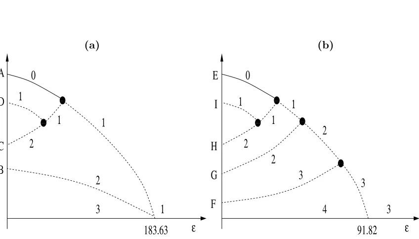
Now we can immediately draw the bifurcation diagram using the following three rules [12, 18]. First a bifurcating branch must have the isotropy subgroup which is a subgroup of the isotropy subgroup of the primary branch; secondly dimensions of unstable manifolds have to match at a bifurcation point to satisfy the principle of exchange of stability, and thirdly atε= 0; the number of nodal domains must increase from one bifurcation point to the next.
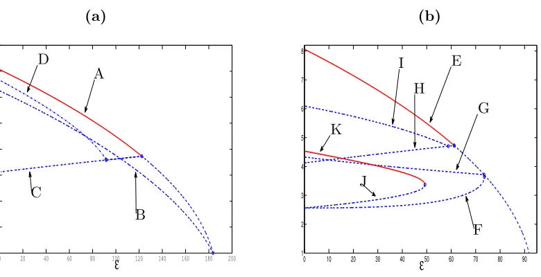
With these rules there is only one way to construct the bifurcation diagram; see Figure 2 (a) and (b), where the y-axis is not to any scale, and is only intended to make clear the end-points of various branches atε= 0. These figures show the bifurcation structure arising from bifurcations of the zero solution.
We would like to make the following observations. The stable non-zero-mean branches cor-responding to the orbit K have to arise through a saddle-node bifurcation. Numerically, this happens at a value of epsilon ≈ 49.294 that is smaller than the value ε4 = 122.432 at
Name Orbit length Σx (0,0,0,0) 1 D4×Z2
(1,1,1,1) 2 D4 A (-1,1,1,-1) 4 hf, p2mi B (1,0,-1,0) 4 hmp2, f pi C (0,0,1,1) 8 hfi D (0,-1,1,1) 16 hIi
Name Orbit length Σx
E (-1,1,-1,1) 2 hpm, f pi F (0,1,0,0) 8 hf pi G (1,0,0,-1) 8 hmfi H (0,1,0,1) 4 hp2, f pi
[image:9.612.80.477.151.260.2]I (0,1,-1,1) 8 hf pi J (0,1,1,1) 8 hf pi K (-1,1,1,1) 8 hf pi
Table 2: Steady states for N = 4, the length of the orbits and isotropy subgroups Σx. We have separated the solutions into the homogeneous states, those connected with the first and second bifurcation ofu = 0 and the two solutions connected by a saddle-nodeJ and K. See also Figure 2.
(a) (b) 0 0 1 1 00 00 11 11
ε
2
1
0
1
1
B
C
1
A
D
2
3
183.63
0 0 1 1 0 0 1 1 0 0 1 1 0 0 1 191.82
ε
4
3
3
3
2
2
1
2
1
1
0
E
I
H
G
F
[image:9.612.90.514.372.614.2](a) (b)
0 20 40 60 80 100 120 140 160 180 200 1
1.5 2 2.5 3 3.5 4 4.5 5
ε
A
B C
D
0 10 20 30 40 50 60 70 80 90 1
2 3 4 5 6 7 8
ε
E
F G H
I
[image:10.612.112.502.102.302.2]J K
Figure 3: Numerically computed bifurcation diagram from the zero solution from the first (a) and second (b) bifurcation points. Solid lines represent stable and broken lines unstable unstable solutions respectively. We indicate above each branch the dimension of the unstable manifold. We show the homogeneous solutions or the orbitsJ and K connected by a saddle-node bifurcation on (b). Compare to the theoretical prediction in Figure 2.
computed diagram. We will see the equivalents of these statements in higher dimensional discretisations.
Finally, we did not perform a Liapunov–Schmidt calculation to determine the order of bifur-cations at the double eigenvalue point ε= 183.63, but the opposite assignment of stabilities cannot be reconciled with the above rules of bifurcation.
3.2 The case of N = 32
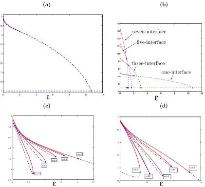
Though an analysis similar to that in the case of N = 4 can be attempted here, the numbers of orbits are astronomical, and we rely on our numerical continuation method, the results of which match exactly the predictions of the analysis in the caseN = 4. In Figure 4 we plot in (a)–(d) sample solution branches of the bifurcation diagram withN = 32. If we start with a large value of εwe see in (a) and (b) the first bifurcation arises at ε≈10.64 as predicted by the theory in Table 2. In (a) we show the continuation of the zero mean one-interface which undergoes a pitchfork bifurcation atǫ≈2.012. In (b) we have plotted the one-, three-, five- and seven interfaces and their stabilization. In (c) we show details of the bifurcation structure close to the pitchfork at ε ≈ 2.012 (note for clarity one branch of the pitchfork seen in (a) is not plotted). Asα → 0.5, the saddle-node bifurcation points converge to ε3,2.
This structure is repeated for the othern-interface solutions and is illustrated in (d) for the three-interfaces solutions. Here we see that the zero-mean one-interface solution branches stabilize atε3,2 ≈2.012. Below we will formulate a conjecture concerning the limiting value
which we callε0
4
The limiting problem and conclusions
It is not hard to prove (see for example [3]) that if ε >1, steady state solutions of (4) are continuous, since the function −εu+f(u) is monotone. Hence it is interesting to understand when the solutions lose continuity (certainly, for ε= 0 there are no non-constant continuous solutions).
The non-trivial stable one-interface zero-mean solution branches (α = 0.5) that originate at
ε= 0 were investigated in detail as we change N. If we defineM by
M := max j
uj+1−uj
h
then for a C1 function this converges to maxx∈[0,1]|ux| and so we can identify where the solution is continuous.
Figure 5 plots in (a) M against ε along a branch of one-interface zero-mean solutions for
N = 2p, p= 4,5,6,7,8,9,10. If we let εd1 be the value of ε at which this branch of solutions becomes discontinuous, then this figure suggestsεd
1 = 1. This is supported in (b) which shows
for differentεconvergence of the derivative M withN on a log log scale.
Furthermore the loss of continuity appears to coincide with the loss of stability. In Figure 6 we show numerically that the bifurcation values converge toε0
1 =ε02 =ε03= 1 as N → ∞.
Now we can collect our observations and form two conjectures. First we consider the zero-mean interface branches. Letε0mbe the value at which the zero-mean 2m−1-interface solution becomes stable. Let εd
m be the value ofεat which this branch becomes discontinuous. Then we have
Conjecture 1: ε0m=εdm.
We can prove a very weak form of this conjecture form= 1. From the results of [3] it follows that discontinuous stationary solutions will exist for anyǫsuch that the function
g(u) :=−εu
Z 1
0
J(s)ds+f(u)
is non-monotone. On the other hand, from Theorem 2.1 of [6] it follows if g(u) is monotone, there are no nonconstant minimizers of the energy functional (3). Hence we have εs1 ≤ εd1. However we do not have the inequality the other way.
We now consider the saddle-node bifurcation of the non–zero mean interface solutions. Now, letus be a branch of 2m−1-interface stable solutions of (4) with mean s, and letεb,sm be the value of ε at which the saddle-node bifurcation giving rise to the branch occurs. Then we have
Conjecture 2: lim s→0ε
b,s m =ε0m.
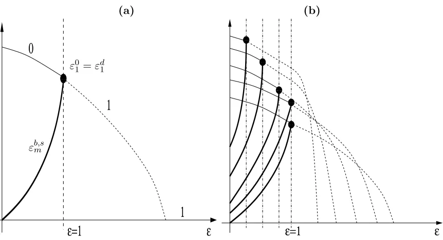
These two conjectures, if true, would lead to the bifurcation picture sketched in Figure 7. In (a) we plot the zero-mean one-interface branch and have indicated the continuum of saddle– node bifurcations εs
1 that approach the bifurcation at εs1 = εd1 = 1. In (b) we indicate the
first four branches of the infinite number that bifurcate from zero, the branches of associated saddle-node bifurcations and here we have that lims→0εb,sm = ε0m = εdm. In addition our numerical investigation seems to indicate thatεs
1 =εd1 = 1 =εs2 =εd2.
parameter space with one, three and five interfaces and so on. In conclusion the diffusion coefficientεdetermines the number and type of stable solutions.
References
[1] P. Bates and F. Chen. Periodic travelling waves for a nonlocal integro-differential model. Electronic Journal of Differential equations, 1999(26):1–19, 1999.
[2] P. W. Bates and A. Chmaj. A discrete convolution model for phase transitions. Arch.
Ration. Mech. Anal., 150(4):281–305, 1999.
[3] P. W. Bates, P. C. Fife, X. Ren, and X. Wang. Travelling waves in a convolution model for phase transitions. Archive for Rational Mechanics and Analysis, 138(2):105–136, July 1997.
[4] S. K. Bhowmik.Numerical approximation of a nonlinear partial integro-differential equa-tion. PhD thesis, Heriot-Watt University, Edinburgh, UK, April, 2008.
[5] F. Chen. Uniform stability of multidimensional travelling waves for the nonlocal Allen-Cahn equation. Fifth Mississippi State Conference on Differential Equations and Com-putational Simulations, Electronic Journal of Differential Equations, Conference 10:109– 113, 2003.
[6] A. Chmaj and X. Ren. The nonlocal bstable equation: stationary solutions on a bounded interval. Electr. J. Diff.eqns., Vol. 2002(02):1–12, 2002.
[7] J. Coville and L. Dupaigne. Propagation speed of travelling fronts in non local reaction-diffusion equations. Nonlinear Analysis, 60:797–819, 2005.
[8] K. Deng. On a nonlocal reaction-diffusion population model.DCDS series B., 9(1):65–73, 2008.
[9] D. B. Duncan, M. Grinfeld, and I. Stoleriu. Coarsening in an integro-differential model of phase transitions. Euro. Journal of Applied Mathematics, 11:511–523, 2000.
[10] P. C. Fife. Models of phase separation and their Mathenmatics. Electronic Journal of Differential Equations, 48:1–26, 2000.
[11] P. C. Fife. Well-posedness issues for models of phase transitions with weak interaction. Nonlinearity, 14:221–238, 2001.
[12] M. Golubitsky, I. N. Stewart, and D. G. Schaeffer.Singularities and Groups in Bifurcation
Theory: Vol. II. Springer-Verlag, New York, 1988.
[13] W. Govaerts. Numerical bifurcation analysis for ODEs. Journal of Computational and
Applied Mathematics, 125(3):57–68, 10 2000.
[14] W. J. F. Govaerts. Numerical Methods for Bifurcations of Dynamical Equilibria. SIAM, Philadelphia, 2000.
[16] M. Grinfeld and I. Stoleriu. Truncated gradient flows of the van der Waals free energy. Electron. J. Diff. Eqns., Vol. 2006(152):1–9, 2006.
[17] T. Hartley and T. Wanner. A semi–implicit spectral method for stochastic nonlocal phase-field models. DCDS, 25(2):399–429, Oct. 2009.
[18] R. B. Hoyle. Pattern Formation : an Introduction to Methods. Cambridge University Press, Cambridge, 2006.
[19] V. Hutson and M. Grinfeld. Non-local dispersal and bistability. Euro. Journal of Applied
Mathematics, 17:211–232, Feb 2006.
[20] Garcia Melian J. and J. D. Rossi. logistic equation with refuge and nonlocal diffusion.
Communications on Pure and Applied Analysis, 8(6):2037–2053, 2009.
[21] J. Medlock and M. Kot. Spreading disease: integro-differential equations old and new.
Mathematical Biosciences, 184:201–222, 2003.
[22] Z. Mei. Numerical Bifurcation Analysis for Reaction-Diffusion Equations. Springer, 2000.
[23] K. E. Morrison. Spectral approximation of multiplication operators. New York Journal
of Mathematics, 1:75–96, 1995.
[24] J. D. Rossi and A. F. Pazoto. Asymptotic behaviour for a semilinear nonlocal equation.
Asymptotic Analysis, 52(1-2):143–155, 2007.
(a) (b)
0 2 4 6 8 10 12
1 1.5 2 2.5 3 3.5 4 4.5 5
ε
0 2 4 6 8 10 120 2 4 6 8 10 12 14 16 18
ε
seven-interface
five-interface
three-interface
one-interface
(c) (d)
0 0.5 1 1.5 2 2.5
3.8 4 4.2 4.4 4.6 4.8 5
ε
α=0.2
α=0.3
α=0.5
α=0.4
α=0.1
0 0.5 1 1.5
6.5 7 7.5 8 8.5 9
ε
α=0.1
α=0.2 α=0.3
α=0.4
α=0.5
Figure 4: (a) Continuation of the zero-mean one-interface (α = 0.5) solution branch. When
[image:14.612.85.506.172.556.2](a) (b)
0 0.5 1 1.5 2 2.5 3 3.5
0 200 400 600 800 1000 1200 1400 1600 1800 2000
ε
1024 512 256 128 64 32 16
101 102 103 104
101 102
103 104
Log(N)
Log(max(|u
x
|))
[image:15.612.86.517.114.344.2]ε=[0, .25, .5, .75, 1, 1.1, 1.2, 1.25]
Figure 5: In (a) we show the maximum of|ux|in [0,1] of the solution u(x) for one-interface initial data with ±1 andα= 0.5. In (b) we see maxx(ux) for different system sizes for some particular ε’s with system size as the x-axis with a clear change in behaviour at ε= 1.
(a) (b)
200 400 600 800 1000
0.8 1 1.2 1.4 1.6 1.8 2
N
one interface three interface five interface seven interface
ε
0 m
102 103
10−4 10−2 100
N
one interface
three interface
five interface
seven interface
ε
0 m
−
z
[image:15.612.89.503.440.667.2](a) (b)
ε=1
0 0 1 1
ε
0
1
1
εb,smε0 1 =εd1
0 0 1 1 0 0 0 1 1 1
0 0 1 1 0 0 0 1 1 1
0 0 1 1
ε
ε=1
Figure 7: (a) Proposed bifurcation diagram for the one-interface solutions in the N = ∞
[image:16.612.88.519.263.497.2]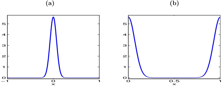
![Figure 5: In (a) we show the maximum of |particularinitial data withux| in [0, 1] of the solution u(x) for one-interface ±1 and α = 0.5](https://thumb-us.123doks.com/thumbv2/123dok_us/1681387.121531/15.612.89.503.440.667/figure-maximum-particularinitial-data-withux-solution-interface-a.webp)