Vibration-based damage detection in plates by using time series analysis

Vibration Based Damage Detection in Plates by Using Time

Series Analysis

Irina Trendafilova1_{, Emil Manoach}2

1

Department of Mechanical Engineering, University of Strathclyde, Glasgow, UK

e-mail: [email protected]

2

Institute of Mechanics, Bulgarian Academy of Sciences, Sofia, Bulgaria

[email protected]

ABSTRACT.

This paper deals with the problem for vibration health monitoring (VHM) in structures with nonlinear dynamic behaviour. It aims to introduce two viable VHM methods that use large amplitude vibrations and are based on nonlinear time series analysis. The methods suggested explore some changes in the state space

geometry/distribution of structural dynamic response with damage and their use for damage detection purposes. One of the methods uses the statistical distribution of state space points on the attractor of a vibrating structure, while the other one is based on the Poincaré map of the state space projected dynamic response.

In this paper both methods are developed and demonstrated for a thin vibrating plate. The investigation is based on finite element modelling of the plate vibration response. The results obtained demonstrate the influence of damage on the local

dynamic attractor of the plate state space and the applicability of the proposed strategies for damage assessment. The approach taken in this study and the suggested VHM methods are rather generic and permit development and applications for other more complex nonlinear structures.

I. INTRODUCTION AND MOTIVATION

VHM methods are based on the fact that any changes in a structure in turn

introduce changes in its vibration response. The problem for damage diagnosis seeks to extract information about the presence, the location and the extent of damage from the vibration response of the structure. The simplest way to do VHM is using the first several natural frequencies of a structure, which are easy to determine from experiment. But they are global characteristics and thus, in a lot of cases, may remain unaffected by damage and especially by localised damage. Mode shapes are in general more sensitive to damage but they are difficult to measure and/or estimate from measured quantities [1]. Another alternative are the updating methods, which are based on comparison of the measured and the modelled response of a structure. The application of these methods is limited by the need of a precise enough model of the structural vibration response.

The above limitations clearly call for an alternative approach, which emerged and developed in a recent trend in structural VHM. It suggests the use of purely data based methods which make use of the measured structural vibration response signal [2-7]. There are different ways to use the measure structural vibration response. A

straightforward possibility is to use the frequency response functions (FRF’s). Such methods suffer the limitations of the excessively large number of frequency lines in the spectrum, which make any further analysis and application very difficult before any preliminary data reduction is made [8].

of the reasons for using phase space is that nonlinear signals are slightly predictable in time, but they have structure which can be observed in phase space. Such methods are relatively new and insufficiently explored fro structural dynamics and VHM purposes but the existing research proves their capabilities and potential [2-7]. The application of such methods is especially appropriate when the structure is subjected to large

amplitude vibrations, which enhance the influence of any nonlinearities, present in the structure, and as a result the structural vibration response is represented by a nonlinear signal. Under large amplitude dynamic loads even small changes in the structure (like cracks and other local damage scenarios) can have a big effect on the structural response in the time domain, which can give indication for the presence of damage. Damage which induces very small changes in the natural frequencies and the mode shapes may result in phase shifts between the vibration response of the healthy structure and the damaged structure in the time domain.

This study suggests the use of large amplitude vibrations and develops two viable methods for damage diagnosis in structures, which are based on nonlinear time series analysis. Here the methods are developed for a thin squareplate and their capabilities are demonstrated for a thin aluminium plate.

subjected to dynamic loading leading to large amplitude vibrations. In such cases the small deflection plate theory cannot assure the adequate simulation of the plate response and therefore the large deflection plate theory, where the geometrical nonlinearities are included should be used [11,12]. On the other hand, large amplitude vibrations can allow small defects (which will not influence the response in the case of small

deflections in the plate) to affect substantially the dynamic behaviour of the plate and in this way to be easily identified. For the above reasons the geometrically non linear version of the so called Reisner-Mindlin plate theory (the first order plate theory) was used to model the plate behaviour [13,14]. It is out of the scope of this paper to concentrate on the details of this theoryand on the method of the solution of the equation of motion. The governing equations and the idea of the used method for rectangular plates are presented very briefly in the Appendix.

It has been found in several studies that the lower natural frequencies of plates might be insensitive to damage [9,15]. This paper also explores the sensitivity of the first several natural frequencies of the plate to damage but it only confirms the previous findings that the changes in the lower natural frequencies of the plate considered are insufficient to be used as damage indicators. The paper then goes on and examines the difference between the two types of vibration responses (in undamaged state and in the presence of damage) in a state space to extract features that can be used for damage detection and localisation.

introduces and discusses the results of the numerical experiments. The paper finishes with some conclusions.

II. THE STATE SPACE APPROACH AND DAMAGE DETECTION

The concept for state (phase) space representation and reconstruction stems from the dynamical system approach for analysis of non-linear time series. The main idea of this approach is to equip the investigator with tools for analysis and modelling of a system from observed time dependent variables. The application of such an approach for a vibrating system will give us the possibility to reconstruct its dynamic behaviour from its measured vibration response. The application of state space reconstruction is especially appropriate for nonlinearly vibrating structures, when their vibration response is represented by a nonlinear signal. Nonlinear signals have slight predictability in the time and in the frequency domain. The state space reconstruction for a nonlinear signal is like the Fourier transform for linear signal processing- it represents the signal in a new space where it has structure and its structure is easily observable [16,17]. A

vibrating structure can be considered as a dynamic system whose behaviour is described by the following system of differential equations

F(x(t)) x

=

dt d

(1)

vibrating system can be completely reconstructed from measurements [16,17]. So the question is how to reconstruct such a state space from the structural vibration response which is normally represents by a single scalar time dependent variable.Obviously a vibrating structure is a much more complex system and cannot be represented in a one-dimensional space. Takens theorem [16] gives the answer to this question. The theorem proves that if we are able to observe a single scalar quantity s(n), n=1,2…. of some vector function of the dynamic variable x, s(n)=s(g(x(n)), then the dynamics of the system can be unfolded in a space made out of new vectors with components consisting of s(n). These new vectors y

)] ) 1 ( ( ),..., (

), ( [

) s n s n T s n m T

n = + + −

y( (2)

composed simply of time lags of the observation define the motion in an m-dimensional Euclidean space. In particular it is shown that the evolution in time of the points

) 1 ( )

(n →y n+

y follows that of the unknown dynamics ( )x n →x(n+1). This procedure converts the scalar measured series s(n) into a vector series y(n). The new space defined by the vector y is the state space that we were looking for. T and m are known as the time delay and the embedding dimension of the new state space. They have to be properly chosen so that the dynamics of our original system can be completely reconstructed in the state space y. A proper time lag can be chosen using the first minimum of the average mutual information while a sufficient embedding dimension m

rather than a full reconstruction of the vibrating structure, a dimension m=2 is used assuming that it will preserve some of the properties of the vibrating system and some changes introduced by damage will be possible to observe in it.The choice of a proper time lag is discussed later.

Once proper embedding dimension and time lag are chosen, the next question is how to characterise our vibrating structure in the new state space so that we can look for changes caused by damage.

Since the reconstruction of the mapping relation y(t+T)=G(y(t)) is not possible for most dynamic systems the alternative of studying its attractor is chosen. The

attractor is the invariant subset towards which the trajectories of the system converge. It can be characterised by its invariants- the Lyapunov spectrum, the entropy and different dimensions. It can be argued and there is much evidence that these characteristics change with the introduction of damage [2,6,7,19]. But these invariants are difficult to determine from measured data [16,17,19]. An alternative way which overcomes this difficulty is to study the geometry or the distribution of points on the attractor [16]. It can be proven and there is enough evidence that the distribution of points on the attractor and its geometry are rather sensitive to even small changes in the system including damage [4-7].

III. THE PROPOSED METHODS

This piece of research concentrates on studying the distribution of points on the attractor and analysing the effect of damage on some of its properties. The first method suggests to analyse the statistical distribution of points on the attractor, while the other alternative looks at their Poincaré map.

III.1. Statistical distribution of points on the attractor and the effect of

damage on it.

This method suggests to study the statistical distribution of points on the attractor and use it to extract damage sensitive features. One of the advantages of using these statistical characteristics is that they are easy to determine from measured data. Another advantage is that in general the statistical characteristics of a nonlinear system are more robust to noise than any deterministic characteristics. The determination of any

deterministic characteristics ( invariants) of a nonlinear signal from observations is very difficult (if possible at all) and the estimated characteristics could be quite imprecise [16,17].

space points. For the purposes of this method we use acceleration signals only because acceleration is the most common quantity to measure on a vibrating structure. Suppose one measures a long enough acceleration signal. It can be represented by an

acceleration vector a as follows:

n i T t t a a a t a t a t a i i T n T n ,..., 3 , 2 ] ,..., , [ )] ( ),...., ( ), ( [ 1 2 1 2 1 = + = = = − a (3)

where a(ti) are the measured accelerations in the time moments ti,i=1,2….,n,n is

large enough, the superscript [...]T stands for transpose and T is the time lag found as explained above.

From a vector a one can obtain n-1 state space points:

1 ,..., 2 , 1 ] , [ ] ,

[ _{1 2 1}

− = = = ₊ n i a a y

y_{i i} T _{i i} T

i y

(4)

A set of N trajectories yk, k=1,2,…N, is then randomly chosen on the response attractor and NB nearest neighbours are found for each trajectory in the sense of

Euclidean distance, yi_q, i=1,2,…,N,q=1,2,…NB. This set is denoted by Yn,

      = = = N k N q k q n B ,... 2 , 1 ,... 2 , 1 y

Y . The set Yn, n=1,2,…,N.NB =M is used to characterise the

attractor of the response signal.

Now that we have obtained the set of vectors Yn the next task is to characterise the

of the obtained sample Yn. Some of our and other authors’ previous research has shown

that certain statistical characteristics of this distribution might be sensitive to damage [2,3,6,7,19]. For instance the variance and the skewness have been found to show sensitivity to damage in some cases, while other statistical moments turned less sensitive [2,6]. For a multidimensional distribution these characteristics can be defined by the following scalar quantities, which are suggested in [20]

∑ ∑ − − = ∑ ∑ − − = = = = = n i n j T n i n j T M s M 1 3 1 2 1 2 1 2 )] ) [( 1 )] ( ) [( 1 Y (Y S Y Y Y Y S Y Y j i j i σ (5)

where M is the number of points Yn, n=1,...,M, Yis the sample mean vector and S is the sample covariance matrix. Instead of using the values for σ and s one can introduce relative changes compared to the non damaged case. These characteristics are introduced below: n n s n n s s s F F − = − = σ σ σ σ (6)

The above quantities can be used as damage features. The multivariate statistics (5) as well as the damage features (6) can be calculated for each measured time domain signal and they are expected to give reliable results provided the signal is long enough. These quantities will characterise the local dynamic state of the structure close to the point on the structure where the measurement is taken. Here and thereafter local refers to the location on the structure where the measurements are taken. We shall call σ and

local features will give information about the local distribution of state space points and the local damage state of the structure close to the measurement point. If one has more than one measurement points, the above characteristics can be then calculated using all the signals coming from different measurement points. The resulting statistics (5) will then contain information about the distribution of state space points for the whole structure and the damage features (6) will characterise the damage state of the whole structure. We shall call these globalstatistics and global damage features respectively.

Global here and thereafter refers to the structure. The global features will give

information about the damaged state of the whole structure. When damage is introduced in the structure it is expected to affect the local damage features calculated for the measurement points close to the damage more than the global features which are calculated for all the measurement points on the structure. So the local damage features might be used to localise the damage while the global features can be used as global damage features are better to use to detect the presence of damage in the whole structure.

III.2. The Poincaré map

Another way to analyse the nonlinear time domain vibration response in a state space is to use its Poincaré map. The second method suggested here utilises the Poincaré map to extract damage sensitive features.

A standard technique in dealing with phase space of periodically driven oscillators

is to inspect the projection w,dw

dt

 

 

  whenever t is a multiple of the period Τ0=2π/ω and

T0 is a period of the forcing, an eigen period of the system or its multiple. The result of

inspecting the phase projection only at specific times t=kT0 is a sequence of dots,

representing the so-called Poincaré map. The steady-state converging trajectories, which represent the attractor, are usually formed in the phase space and in many cases of nonlinear systems they are very sensitive to any changes in the system.

The idea of the approach presented here is based on the following considerations:

1. A Poincaré map can be interpreted as a discrete representation of the dynamic system in a state space which is one dimension smaller than the original continuous space of the dynamic system. Since it preserves many properties of periodic and quasi-periodic orbits of the original system and has a lower dimension, it is often used for analyzing the original system. 2. The Poincaré maps contain data for the displacements and the velocities of

the structure in a compact form and since these two parameters are expected to be sensitive to damage, these diagrams can be used to detect damage.

When the plate has undergone substantial damage and it is subjected to large amplitude nonlinear vibrations, this leads to changes in the attractor of the vibrating system in the phase space and then the application for damage assessment purposes becomes obvious. Even when the damage is small, and the responses of the damaged and the healthy structure are close to each other, the points from the Poincaré map are easier to use for comparison and identification purposes because the number of this points is not comparable to the enormous number of points in the time-history diagrams.

u d

d i i

i _u i S S I S −

= , (7 a)

(

) (

)

(

) (

)

1 1

2 2 2 2

, 1 , , 1 , , 1 , , 1 ,

1 1

;

p p

N N

u u u u u d d d d d

i i j i j i j i j i i j i j i j i j

j j

S w w w w S w w w w

− −

+ + + +

= =

=

∑

∑

\

where, i=1,2…Nnodes, Nnode is the number of nodes, Np is the number of points in the

Poincaré map and (w w_iju, _iju) and (w_ijd,w_ijd) denote the j-th point in the Poincaré maps in the undamaged and in the damaged state respectively.

A small (close to 0) damage index will indicate no damage, while a big damage index will indicate the presence of a fault at the corresponding location. The above damage index depends on the location of the point on the plate and consequently it is a function of the plate coordinates x and y. One can expect that the maximums of the surface I_id defined by equation (7a) will represent the location of damage in the

structure (x_d,y_d), i.e. ( , ) max{ _id} i d d

d _{x y I}

I =

It is easy to notice that S_iu and S_id (7 b,c) represent the lengths of the lines formed by connecting the dots on the Poincaré maps for the non-damaged and the damaged plate for i-th node, respectively. Therefore the damage index is defined as the relative difference between these two lengths. The logical expectations are that:

2) At the nodes close to the damaged area the introduced damage index I_id (7 a) will be larger than the index for points which are far from the damaged zone. This can be used to localize the detected damage.

It should be noted that the criterion (18) includes an integral measure of the dynamic behaviour of the structure in the total time interval. We would like to mention that our attempts to apply a simpler criterion, e.g. a criterion based on distance between the Poincaré map dots for the damaged and the undamaged state, i.e. :

2 2

, , , ,

1 , ,

;

p u d u d

N

i j i j i j i j

i u u

j i j i j

w w w w

S

w w

=

_{   } 

− −

 

   

= _{ } +_{ } 

    

 

∑

showed completely inability to predict the damage as well as its location.

IV. THE CASE STUDY

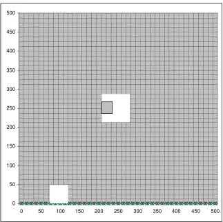
the second damage level the thickness in the corresponding damage zone is reduced to 3mm.

The plate was subjected to a harmonic loading uniformly distributed on the plate surface with different frequencies close to one of the plate’s natural frequencies. Cases when the frequency of excitation is close to one of the first natural frequencies of the systems are interesting and important for this study of a nonlinear system because they often lead to large amplitude vibrations and may result in complex phenomena like beating, quasi-periodic or chaotic vibrations [21,22] . In such regimes vibrating systems are usually quite sensitive to even small changes in the geometry and the physical properties of the structures and this is therefore expected to enhance their sensitivity to damage, even though the changes in the natural frequencies might be negligible. Numerical experiments were carried out for different values of the excitation

frequencies. In the case of central defect (case A) the excitation frequency was chosen equal to ωe=1000 rad/s. In order to show the applicability of the methods for higher frequencies for the case B the excitation frequency was ωe=2000 rad/s. (The first two natural frequencies of healthy plate are ω1=1326.32 rad/s, ω2=2700.3 rad/s ) The amplitude of the harmonic loading was 6 N.

The aim of the following numerical examples performed is to test the suggested procedures to detect and localise damage in the plate.

V. SOME RESULTS

In this paragraph some result for the detection and the localisation of the two damage scenarios described above -the central and the side defect- are discussed.

in the first 10 natural frequencies of the plate. The differences between the frequencies of the intact and the damaged plate do not exceed 2 %. These results were

experimentally confirmed as well. So in this particular case there is obviously a need for an alternative method.

Let us first have a look at the time histories of the plate response for the non damaged and the damaged cases. Figures 2 and 3 give parts of the time histories for the case of central defect and side defect, respectively, compared to those for the non damaged plate. The figures present the time histories for the case of no damage and for the two damage levels. It can be observed that the applied load leads to large amplitude vibrations of the plate. Due to the fact that the excitation frequency is close to one of the first natural frequencies of the plate a beating phenomenon occurs. It can be

appreciated from Figures 2 and 3 that the time histories undergo significant changes with damage. As it is expected the differences for case A of central defect are bigger than the differences for case B of side defect. It can be seen that close to the beginning (t=0) the responses almost coincide (especially for the case B) but then the phase shifts and the differences between the responses increase. For damage level 2 the time histories go still further apart. Another conclusion that can be made from Figures 2 and 3 is that the response signals, especially those which correspond to a damage state, look complex and nonlinear and they are not made of single frequency harmonics. The representation of these signals in the frequency domain confirms this observation. This justifies our motivation to use nonlinear signal analysis methods for the purposes of this investigation.

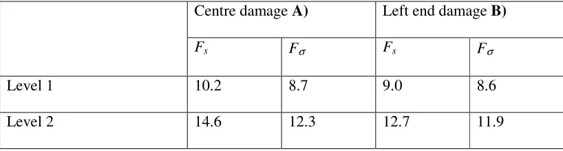
distribution of points on the attractor. Thus if there is no change in the damage state these indexes should be close to 0 while if there is a change in the damage state of the plate these indexes are expected to increase. In this numerical example it was assumed that measurements are taken in a net of 16 equally distributed points that cover the surface of the plate. The global indexes were calculated using the signals obtained in all the 16 points, while the local indexes were calculated for the signals obtained in each one point. Since we don’t assume any preliminary information about the location of damage we shall first use the global indexes to test their use for detection purposes. Table 1 below gives the results for the global indexes for both damage types for the two damage levels. It can be noticed that both damage indexes undergo a certain change, which is smaller for the first damage level and it goes up for the second damage level. The change, especially for the first damage level, is not tremendous, but one should keep in mind that these are the global indexes, which will give the relative change in the statistic for all the measurement points. The signals from points close to the damage will change more than the signals measured in points further from the damage location and therefore some of the differences that contribute to the above damage indexes will be close to 0 and/or very small.

the defect zone is a bit smeared which makes difficult to identify the exact localisation of the damaged zone.

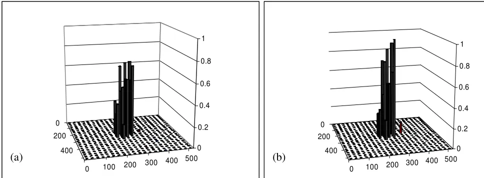
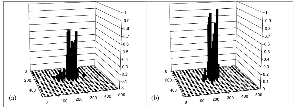
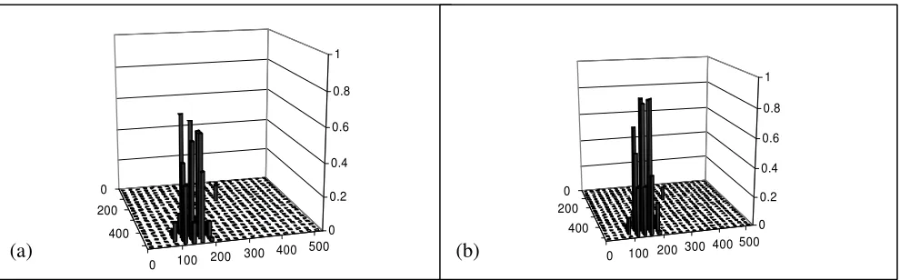
A similar effect was observed for the case of the side defect as well and the next graphs detail the performance of the skewness index only. Figure 6 gives the skewness index Fs for the case of side defect B) for both levels. From figures 4,5 and 6 it can be appreciated that the damage can be localised using the local indexes and that the indexes increase with the increase of damage- they become higher for level 2. Figures 7 and 8 give the local skewness indexes Fs for the cases of central defect A) and side defect B) respectively, for both damage levels, from another perspective as projected on the plate. It can be appreciated that the skewness-based index, gives quite sharp and precise localisation of the damage for both damage levels.

The second method suggests the use of Poincaré maps and the damage index I_id

(equation 7 a) is used to detect and localise damage. To visualize the damage index and to set a threshold for detecting the damage we use the so-called contour plots. A contour plot is a graphical technique for representing a 3-dimensional surface by plotting

constant z slices, contours, on a 2-dimensional plane. That is, given a value for z, lines are drawn that connect the (x,y) coordinates where that z value occurs. The contour plot is an alternative to a 3-D surface plot.

Poincaré maps is a little bigger compared to the influence of the lower level damage (hdamaged =4 mm).

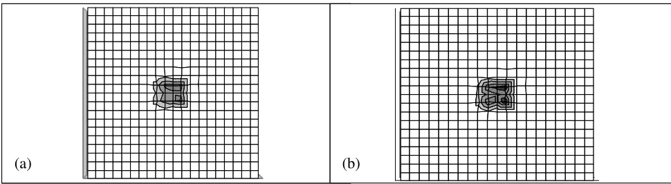
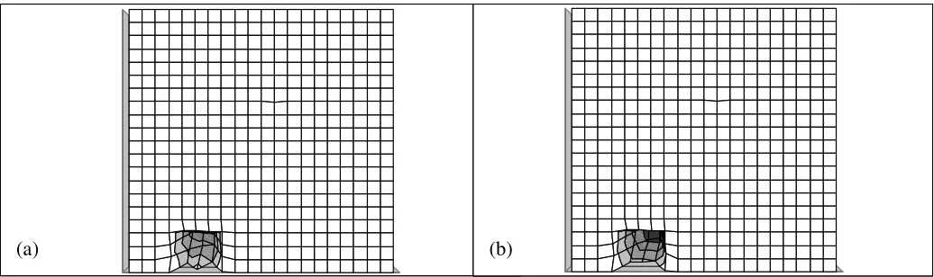
Then the damage index I_idwas calculated for the points from the Poincaré maps for all the nodes and its contour plots were obtained. Figure 11 details the contour plots of I_id for central damage A)for both damage levels. As can be seen from this plots damage A) can be detected and localised quite precisely especially at the second (higher) damage level. The value of the damage index for the second damage level is bigger than the one corresponding to the first damage level . Figure 12 presents similar contour plots for the case of side damage B). The figures detail both damage levels. It can be observed that the plot for the second damage level identifies quite precisely the position of the defect in spite of the fact that the absolute values of the differences in displacements and velocities of the two responses at the nodes of the damaged area are small. The localisation of the damage for the first damage level is not absolutely precise but it is sufficient for many applications.

VI. CONCLUSIONS

(1) Two viable methods for damage detection and localisation are suggested in the paper which are based on a state space representation of the time domain structural response.

(3) Both methods demonstrate quite good abilities to detect and localise damage in the plate. The noise sensitivity of the methods and their capabilities for real measurements still have to be tested.

ACKNOWLEDGMENTS

The authors would like to acknowledge the support of grant 2006/R2-IJP from the Royal Society, UK and of the Bulgarian Research Fund for the partial support through grant

APPENDIX.

Equations of motion of the plate

The geometrically non-linear version of the so called Raisner-Mindlin plate theory was used to describe the dynamic plate behaviour. This theory takes into account the influence of the shear stress and angular rotations on the plate behaviour and gives more adequate results than the classical one especially in the case of thicker plates or when higher frequencies are included into vibrations [13,14].

The equations of motion, according to this theory are as follows:

0 0 xy x x y xy y N N hu x y N N hu y x ρ ρ ∂ ∂ + + = ∂ ∂ ∂ ∂ + + = ∂ ∂ 3 2 3 2 0 12 0 12 xy x x x x

y xy y

y y

M

M h

Q c

x y t

M M _h

Q c

y x t

ψ ρ ψ ∂ ψ ρ ψ ∂ ∂ ∂ ∂ + − + + = ∂ ∂ ∂ ∂ ∂ + − + + = ∂ ∂

2 2 2

1

2 2 2

y x

x y xy

Q

Q w w w w

N N N c hw p

x y x y x y ∂ t ρ

∂

∂ ∂ ∂ ∂ ∂

+ + + + + + = −

∂ ∂ ∂ ∂ ∂ ∂

Here Nx, Ny and Nxy are the stress resultants in the mid-plane of the plate, Mx, My and Mxy

are the stress couples, Qx and Qy are the transverse shear stress resultants, u(x,y,t) and

v(x,y,t) are the in-plane displacements, w x y t

(

)

(

)

(

)

x x y t y x y t

In the present work only fully clamped and in-plane fixed plates are considered, which means that all displacements u, v and w and angular rotations ψ_x andψ_y are zero along the boundaries.

REFERENCES

[1]. Doebling S.W., C.R. Farrar and M.B. Prime, A Summary Review of Vibration-Based Damage Identification Methods, The Shock and Vibration Digest, Vol. 30, No. 2, (1998), pp. 91-105.

[2]. Todd M., J M Nichols, L M Pecora and L Virgin, Vibration-based Damage Assessment Utilizing State Space Geometry Changes: local Attractor Variance Ratio, 2001,Smart Mater. Struct. 10, pp 1000-1008.

[3]. Sohn H. and Farrar C., Damage diagnosis using time series analysis of vibration signals, 2001, Smart Mater. Struct.10 pp 1–6.

[4]. Nichols J.M., Trickey S.T., Seaver M., Damage detection using multivariate recurrence quantification analysis, 2006, Mechanical Systems and Signal Processing 20, pp 421–437.

[5]. Moniz L., Nichols J.M., Nichols C.J., Seaver M., Trickey S.T., Todd M.D., Pecora L.M., Virgin L.N., A multivariate, attractor-based approach to structural health

monitoring, 2005,Journal of Sound and Vibration 283, pp 295–310.

[6]. Trendafilova I., Vibration-based damage detection in structures using time series analysis, 2006, Journal of Mechanical Engineering Science, Proceedings of the Institution of Mechanical Engineers Part C, Volume 220, Number 3, pp 261-272. [7]. Trendafilova I., State space modeling and representation for vibration-based damage assessment, 2003, “Damage Assessment in Structures”, Key Engineering

[8]. C. Zang and M. Imregun, Structural damage detection using artificial neural networks and measured FRF data reduced via principal component projection, 2001, Journal of Sound and

Vibration 242(5), p. 813-827

[9]. Israr A.,. Cartmell M.P, Krawczuk M.,. Ostachowicz W.M, Manoach E., Trendafilova I., Shishkina E.V., Palacz M., On Approximate Analytical Solutions for Vibrations in Cracked Plates, 2006,Applied Mechanics and Materials 5-6, pp 315-322. [10]. Khadem, S.E. & Rezaee, M., Introduction of Modified Comparison Functions for Vibration Analysis of a Rectangular Cracked Plate, 2000, Journal of Sound &

Vibration,236(2), pp. 245-258.

[11]. Manoach, E. Dynamic response of elastoplastic Mindlin plate by mode superposition method, 1993. Journal of Sound and Vibration,162, pp.165-175.

[12]. Manoach. E. Dynamic large deflection analysis of elastic-plastic Mindlin circular plates,1994, International Journal of Non-Linear Mechanics, Vol. 29,pp. 723-735 [13]. Hutchinson, J. R., Wave propagations using Mindlin plate theory, 1982,Current Advances in Mechanical Design and Production, Second Cairo University MDP

Conference, 27-29 December, 1982, Cairo, Egypt, pp. 17-24

[14]. Hutchinson , J. R, Response of a free circular plate to a central transverse load.

1988, J. Sound and Vibration, 123, pp. 129-143

[15]. Lazarov B., Trendafilova I., An Investigation on Vibration-Based Damage Diagnosis in Thin Plates, 2004, Structural Health Monitoring 2004, Proc. IInd

European Workshop, Munich, July 2004, pp 76-81.

[18]. Fraser A.M. and Swinney H.L, Independent coordinates for strange attractors, 1986,

Phys. Rev A, pp 1134-1140

[19]. Mathew J., Some Recent Advances in Signal Processing for Vibration Monitoring,

1997, Proc. Fifth Internat. Congress Sound and Vibration Adelaide, South Australia,

pp 903-918.

[20]. Mardia, K.V., Measures of multivariate skewness and kurtosis with applications.

1970, Biometrika57, 519-530.

TABLE AND FIGURE CAPTIONS

Table 1. Change in the damage indexes in per cent for the two damage levels in the two damage zones

Figure 1. Plate and defects

Figure 2. Time histories for central defect (Case A) black line –undamaged plate; blue line – level 1, red line -level 2. ;. Excitation frequency ωe=1000 rad/s, p = 6 N

Figure 3. Time histories for side defect (case B) black line –undamaged plate; red line -level 1; blue line –level 2. Excitation frequency ωe=2000 rad/s, p = 6 N

Figure 4. Local damage index Fs for central defect (a) level 1, (b) level 2

Figure 5. Local damage index Fσ for central defect (a) level 1, (b) level 2

Figure 6. Local damage index Fs for side defect (a) level 1, (b) level 2

Figure 7. Another perspective of the local index Fs for central defect (a) level 1, (b) level 2

Figure 8. Another perspective of the local index Fs for side defect (a) level 1, (b) level 2

Figure 9. Poincaré map of the centre of the plate in the case of central damage . Black dots – undamaged plate. Blue dots – level 1, Red dots – level 2.

Figure 10. Poincaré map of the centre of the plate in the case of side damage. Black dots – undamaged plate. Blue dots – level 1, Red dots – level 2..

Figure 11. Contour map of damage index Id for central damage (Case A), (a) level 1; (b) –level 2

Centre damage A) Left end damage B)

Fs Fσ Fs Fσ

Level 1 10.2 8.7 9.0 8.6

Level 2 14.6 12.3 12.7 11.9

0 50 100 150 200 250 300 350 400 450 500

0 50 100 150 200 250 300 350 400 450 500

0.0 1.5

t, sec

-0.012 0.000 0.012 0.024

w

,m

0.0 1.5 time, s

-0.005 0.000 0.005 0.010

w

,

m

Figure 4. Local damage index Fs for central defect (a) level 1, (b) level 2 0

200

400

0 100 200 300

400 500 0 0.2

0.4 0.6 0.8 1

0 200

400

0 100 200 300

400 500 0

0.2 0.4 0.6 0.8 1

Figure 5. Local damage index Fσ for central defect (a) level 1, (b) level 2 0

200

400

0 100 200

300 400 500

0 0.1

0.2 0.3 0.4 0.5 0.6 0.7 0.8 0.9 1

0

200

400

0 100 200

300 400 500

0 0.1 0.2 0.3 0.4 0.5 0.6 0.7 0.8 0.9 1

Figure 6. Local damage index Fs for side defect (a) level 1, (b) level 2 0

200

400

0 100 200 300 400 500

0 0.2 0.4 0.6 0.8 1

0 200

400

0 100 200300 400 500 0 0.2 0.4 0.6 0.8 1

Figure 7. Another perspective of the local index Fs for central defect (a) level 1, (b) level 2

Figure 8. Another perspective of the local index Fs for side defect (a) level 1, (b) level 2

-0.008 0.000 0.008 displecemnts, m

-5 0 5 10 15

v

e

lo

c

it

y

,

m

/s

-0.004 0.000 0.004 displacements , m

-8 -4 0 4

v

e

lo

c

it

y

m

/s

Figure 11. Contour map of damage index Id for central damage (Case A), (a) level 1; (b) –level 2

(a) _(b)

-0.2 -0.1 0 0.1 0.2

-0.2 -0.1 0 0.1 0.2

0.06 0.065 0.07 0.075 0.08 0.085 0.09 0.095

-0.2 -0.1 0 0.1 0.2 -0.2

-0.1 0 0.1 0.2

0.1 0.105 0.11 0.115 0.12 0.125 0.13 0.135 0.14 0.145 0.15

-0.2 -0.1 0 0.1 0.2 -0.2

-0.1 0 0.1 0.2

0.105 0.11 0.115 0.12 0.125 0.13 0.135 0.14 0.145

-0.2 -0.1 0 0.1 0.2 -0.2

-0.1 0 0.1 0.2

0.14 0.15 0.16 0.17 0.18 0.19 0.2 0.21 0.22 0.23 0.24 0.25

Figure 12. Contour plots for the case of side damage. (a) -level 1,(b)- level 2