Microscopic activity patterns in the naming game

City, University of London Institutional Repository

Citation

: Dall'Asta, L. and Baronchelli, A. (2006). Microscopic activity patterns in the

This is the unspecified version of the paper.

This version of the publication may differ from the final published

version.

Permanent repository link:

Link to published version

: http://dx.doi.org/10.1088/0305-4470/39/48/002

Copyright and reuse:

City Research Online aims to make research

outputs of City, University of London available to a wider audience.

Copyright and Moral Rights remain with the author(s) and/or copyright

holders. URLs from City Research Online may be freely distributed and

linked to.

City Research Online: http://openaccess.city.ac.uk/ [email protected]

arXiv:cond-mat/0606125v1 [cond-mat.dis-nn] 5 Jun 2006

Microscopic activity patterns in the Naming Game

Luca Dall’Asta

Laboratoire de Physique Th´eorique (UMR du CNRS 8627),

Bˆatiment 210, Universit´e de Paris-Sud, 91405 ORSAY Cedex (France)

Andrea Baronchelli

Dipartimento di Fisica, Universit`a “La Sapienza” and SMC-INFM,

P.le A. Moro 2, 00185 ROMA, (Italy)∗

Abstract

The models of statistical physics used to study collective phenomena in some interdisciplinary

contexts, such as social dynamics and opinion spreading, do not consider the effects of the memory

on individual decision processes. On the contrary, in the Naming Game, a recently proposed

model of Language formation, each agent chooses a particular state, or opinion, by means of a

memory-based negotiation process, during which a variable number of states is collected and kept

in memory. In this perspective, the statistical features of the number of states collected by the

agents becomes a relevant quantity to understand the dynamics of the model, and the influence

of topological properties on memory-based models. By means of a master equation approach,

we analyze the internal agent dynamics of Naming Game in populations embedded on networks,

finding that it strongly depends on very general topological properties of the system (e.g. average

and fluctuations of the degree). However, the influence of topological properties on the microscopic

individual dynamics is a general phenomenon that should characterize all those social interactions

I. INTRODUCTION

Language Games are a class of simple models of population dynamics conceived to

repro-duce the processes involved in linguistic pattern formation inside a population of

individu-als [1, 2]. They have been profitably used in order to understand the origin and the evolution

of language [3], and have found an important field of application in Artificial Intelligence,

where the ultimate goal consists in modeling the self-organized collective learning processes

in populations of artificial agents [4, 5]. Recently, on the basis of these ingredients, a model

called Naming Game has been put forward as a simple example of collective dynamics

lead-ing to the self-organized emergence of a communication system (i.e. llead-inguistic conventions)

in a population of interacting agents [6, 7]. The original definition of the model considers

a population of agents that assign names to an object, trying to agree on a unique shared

name by means of pairwise negotiations. The Naming Game may be applied to different

contexts. For instance, it may be used to model the opinion spreading in a population of

individuals that interact by means of negotiation, rather than imitation (as in the Voter

model [8]). The concepts of memory and feedback on which the Naming Game is based are

quite new in social dynamics and in statistical mechanics as well. They are at the origin of

very interesting dynamical properties, some of them have motivated the present work. In

particular, we will focus on the role of agents’ memory, by means of which an agent can

store several different states (or words, opinions, etc.) at the same time. The aim of this

work is to provide a detailed statistical description of the internal dynamics of single agents

in the Naming Game, studying their relation with the collective behavior of the model in

its different dynamical regimes.

As many other models of social interaction, the Naming Game is a non-equilibrium model

in which the system eventually reaches a stationary state. The dynamical evolution of these

systems is usually characterized by a temporal region in which the system reorganizes itself

followed by the sudden onset of a very fast convergence process induced by a symmetry

breaking event. The Naming Game presents this type of dynamics when the agents are

embedded in a mean-field like topology, i.e. a complete graph, and complex networks with

small-world property, that are undoubtedly the most realistic cases for models of social

interaction.

0 50000 1e+05 1.5e+05 0

5000 10000

N w

(t) MFER

BA

0 50000 1e+05 1.5e+05

0 200 400 600

Nd

(t)

0 50000 1e+05 1.5e+05

t

0 0.5 1

S(t)

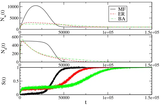
FIG. 1: Global behavior of the Naming Game on different topologies. The complete graph

(mean-field case) is compared to Erd¨os Renyi and Barab`asi-Albert graphs, both with average degree

hk_{i= 10. In all cases, after an initial spreading of the different states, the dynamics goes through}

a period in which different states (whose total number isN_d(t_{)) are exchanged among the agents.}

Thus, the total number of states, N_w(t_{), grows till a maximum and then start decreasing due to}

successful interactions which eventually lead the system to converge (N_d(t_{) = 1,} N_w(t_{) =} N_).

Finite connectivity allows for a faster initial growth in the success rate,S₍t_{). However, small-world}

properties give rise to the same exponential convergence observed in the fully connected graph.

Data refers to populations ofN _{= 1000 agents.}

agents activity allows to investigate the connection between the learning process of the

agents[18] and the topological properties of the system. Interestingly, it turns out that, far

from the convergence process, the shape of the distribution of the number of states stored

by an agent, i.e. its memory size, depends on purely topological properties of the system

(i.e. the first two moments _hk_i and _hk2_{i of the degree distribution). In particular, we}

show analytically, by means of a master equation approach, that homogeneous graphs yield

exponential distributions, while heterogeneous networks, characterized by large fluctuations

of the agents degree, give rise to half-normal distributions.

During the convergence process, on the other hand, the master equation approach is still

appropriate to describe agents internal dynamics, but with qualitatively different results.

All these systems tend to develop a power-law memory-size distribution, that is a signature

(called ‘mean-field’ case). In other topologies, the cut-off sets in too early for the power-law

to be observed.

Therefore, the analytical and numerical study of the memory-size distributions provides

deep insights on the influence of the topology in the dynamics of the Naming Game.

More-over, the new findings are complementary to those already known from the analysis of global

observables, and allow for a deeper understanding of the observed phenomena.

The paper is organized as follows. The next section is devoted to the description of

the Naming Game model. Section III contains the main numerical results concerning the

internal dynamics of individual agents in the Naming Game. In section IV, the problem of

determining agents internal dynamics is faced using a master equation approach. Section V

is devoted to illustrate in details some interesting cases. Conclusions on the relevance of the

present work are reported in section VI.

II. THE MODEL

We consider the minimal model of Naming Game (NG) proposed in Ref. [7]. A population

of N identical agents are placed on the vertices of a generic undirected network, while the

edges identify the possible interactions between them. An agent disposes of an internal

inventory, in which it can store an a priori unlimited number of states. As initial conditions

we require all inventories to be empty. At each time step, a pair of neighboring agents is

chosen randomly, one playing as “speaker”, the other as “hearer”, and negotiate according

to the following rules:

• the speaker selects randomly one of its states and conveys it to the hearer;

• if the hearer’s inventory contains such a state, the two agents update their inventories so as to keep only the state involved in the interaction (success);

• otherwise, the hearer adds the state to those already stored in its inventory (failure).

The collective behavior of the system on different networks has been largely studied in

Refs. [9, 10]. In particular, it turns out that essential quantities to describe the convergence

process are the total number of states present in the system, Nw(t), the number of different

at a given time. In Figure 1 curves relative to complete graph (mean-field), Erd¨os-Renyi

(ER) homogeneous random graph and Barab`asi-Albert (BA) heterogeneous network are

reported (see Refs. [11, 12] for reviews of the networks models). In the fully connected

graph the process starts with an initial moderately fast (linear with time) spreading of states

throughout the system followed by a longer period (O(N1.5_{)) in which states are exchanged}

among the agents. The total number of states then reaches a maximum and starts decreasing

slowly till a point in which an super-exponential convergence leads the population to the

adsorbing configuration in which all agents have the same unique state. On low-dimensional

lattices and hierarchical structures, on the other hand, the model converges very slowly,

and the reason is related to the formation of many different local clusters of agents with

the same unique state, growing by means of coarsening dynamics [13]. Finally, in the case

of networks with finite average connectivity (sparse graphs), the initial dynamics is similar

to that registered in low-dimensional regular structures, but the small-world property (i.e.

average inter-vertex distance scaling as logN and presence of shortcuts connecting otherwise

distant regions) boosts up the convergence process restoring the fast mean-field like cascade

effect leading the system towards the global agreement.

The present work, however, is addressed to study this model from a different and

comple-mentary point of view, focusing on the activity patterns of single agents. The next section

is devoted to show some numerical results on the individual dynamics.

Before proceeding, a remark is in order. In heterogeneous networks, highly connected

nodes (hubs) play a different role in the dynamics compared to low degree nodes. Indeed,

as already pointed out for the Voter model [14], the asymmetry of the NG interaction

rules becomes relevant when the degree distribution of the network, pk, has long tails.

When selecting the two interacting agents, the first node is thus chosen with probability

pk, while the hearer is chosen with probability qk = kpk/hki. Then the high-degree nodes

are preferentially chosen as hearers, if the first extracted node is the speaker. We adopt

this selection criterion, called direct Naming Game, since it fits realistic speaker-hearer

interactions naturally. However other strategies are possible: one could first select the

hearer and then the speaker (reverse NG), or more neutrally, an edge could be selected

and the role of speaker and hearer assigned with equal probability among the two nodes

III. NUMERICAL RESULTS ON AGENTS ACTIVITY

In this section, we study numerically the activity of an agent focusing on the dynamics of

its memory or inventory size, i.e. the number of states nt stored in the inventory of a node

at the time t. In particular, the present analysis is conceived for populations on which we

cannot clearly identify a coarsening process leading to the nucleation and growth of clusters

containing quiescent agents (e.g. complete graph, homogeneous and heterogeneous random

graphs, high-dimensional lattices, etc.) [9, 10, 13].

Complex networks represent typical examples of such topological structures. In other

topologies, such as in low-dimensional lattices, the agents internal activity is limited by the

small number of words locally available. An example of the different activity patterns in

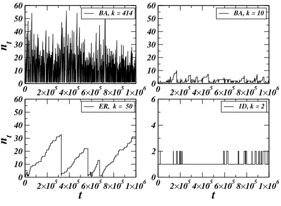
different topologies is reported in Fig. 2. Top panels show the different level of activity

displayed by low and high degree nodes in a BA heterogeneous network. The hubs are more

active, being preferentially chosen as hearers, and they may reach larger inventory sizes

(memory). In homogeneous networks (bottom-left panel) all agents display approximately

the same level of activity. In this case we reported an ER random graph with rather large

average degree, so that the inventory may reach moderately large sizes. It is possible to verify

with a magnification of the scales that the structure of the peaks is the same for all networks.

The only topology displaying clearly different results is the regular one-dimensional lattice

(bottom-right panel), in which the inventory size does not exceeds 2 because of the coarsening

process [13].

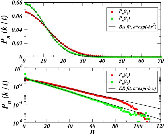
A quantity that clearly points out the statistical differences in the activity of the nodes

depending on both their degree and the topological structure of the network is the probability

distribution_Pn(k|t) that a node of degreek has a numbern of states in the inventory at the

time t. The distribution is computed averaging over the class of nodes of given degree k at

a fixed time t. Fig. 3 displays typical inventory size distributions for the Naming Game on

complex networks computed in the reorganization region that precedes the convergence. The

top panel of Fig. 3 reports_Pn(k|t) for the case of highly connected nodes in a heterogeneous

network (the Barab´asi-Albert network), whereas the bottom panel shows the same data for

nodes of typical degree in a homogeneous network (the Erd¨os-R´enyi random graph). From

the comparison of the curves for different temporal steps (in the reorganization region),

0 _2×105

4×1056×1058×1051×106 0 10 20 30 40 50 60 n t

BA, k = 414

0 _2×105

4×1056×1058×1051×106 0 10 20 30 40 50 60

BA, k = 10

0 _2×105

4×1056×1058×1051×106

t 0 10 20 30 40 50 60 n t

ER, k = 50

0 _2×105

4×1056×1058×1051×106

t

0 2 4 6

1D, k = 2

FIG. 2: Examples of temporal series of the number of states at a given node. Top) Series from

a Barab´asi-Albert (BA) network with N _{= 10}4 _{nodes and average degree h}k_{i = 10, for nodes of}

high degree (e.g. k_{= 414) and low degree (e.g.} k_{= 10). Bottom) Series for nodes in Erd¨os-R´enyi}

random graph (N _{= 10}4_,hk_{i= 50) and in a one-dimensional ring (}k_{= 2).}

considerably in time; the time t enters in the distributions as a simple parameter governing

their amplitude and the position of the cut-off.

Moreover, in homogeneous networks the shape of the distribution does not actually

de-pend on the degree of the node, since all nodes have degree approximately equal to the

average degree _hk_i. In the heterogeneous networks a deep difference exists between the

be-havior of low and high degree nodes. Low degree nodes have no room to reach high values

ofn, thus their distribution has a very rapid decay (data not shown); for high degree nodes,

on the contrary, the distribution extends for more than one decade and its form is much

clearer.

Apart from the behavior of low degree nodes, it is clear that the functional form of the

distribution_Pn(k|t) is different in homogeneous and heterogeneous networks. Homogeneous

networks are characterized by exponential distributions, while high degree nodes in

het-erogeneous networks present faster decaying distributions, that are well approximated by

half-normal distributions (i.e. with Gauss-like shape).

Both cases of homogeneous and heterogeneous networks appear different from that of

0 10 20 30 40 50 60 70 0

0.02 0.04 0.06 0.08

P

(k | t)

P_n(t₁) P

n(t2)

BA fit, a*exp(-bx2)

0 20 40 60 80 100 120

n

10-6

10-4

10-2

100

P

(k | t)

P_n(t₁) P_n(t₂)

ER fit, a*exp(-b x)

FIG. 3: Parametric dependence on time of the distribution of the number of states: the time has the

effect of deforming the shape of the distributions, but does not change their functional description.

Top) BA graph of N _{= 10}4 _{nodes with h}k_{i = 10. Only the set of nodes with} k > _{150 (hubs) is}

monitored. Histograms come from measurements at different times t_{1 and} t_{2 with}t₂₋t_{1 = 5}.₁₀5

time-steps. Bottom) ER graph of N _{= 10}4 _{nodes and h}k_{i = 10. Measures refer to to the set of}

nodes withk >_70. t₂₋t_{1 = 4}.₁₀5 _time-steps.

a complete graph and, during the reorganization, the inventory size distribution is given

by the superposition of an exponential and a delta function peaked around n _∼ √N. The

reason of these differences will be elucidated in the next sections by means of an analytical

approach to the problem.

In contrast with the previous reorganization region, the main global quantities describing

the dynamics accelerate when the system is close to the convergence: Nw(t) converges to N,

whileNd(t) andS(t) go to 1, all with a super-exponentially fast process. Nevertheless, even

in this region, the temporal scale of the global dynamics is much slower than that of agents

activity, thus the fixed-time inventory size distribution _Pn(k_|t) is still a significant measure

of the local activity. In this case, the mean-field presents a more interesting phenomenology

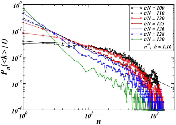
compared to sparse complex networks. Fig. 4 shows that, near the convergence, the complete

graph develops a power-law inventory size distribution, with an exponential cut-off at n _≃

√

100 101 102

n

10-4

10-3

10-2

10-1

100

P

(<k> | t)

t/N = 100 t/N = 110 t/N = 120 t/N = 125 t/N = 126 t/N = 128 t/N = 130 n-b, b ≈ 1.16

FIG. 4: Inventory size distribution for the Naming Game on the complete graph during the

con-vergence process. At the beginning the peak atn_∼√N _{gives way to a power-law, with exponent}

approximately ₋1, that rapidly becomes more and more steep at low values of n_{. The numerical}

data are obtained from a single run of the Naming Game on a complete graph of N _{= 10}4 _nodes,

monitoring the whole temporal region of convergence. Note that we report single run experiments

since the temporal fluctuations of the convergence process are rather large (see Ref. [7]), so that

averaging over many runs may alter the real value of the power-law exponent.

the cut-off moves backwards to 1.

Similar power-law behaviors are not observed in any other topology even if it should be

expected on homogeneous random graphs that, in the limit of large average connectivity,

tend to the complete graph. Numerical simulations instead show that, in the region of

convergence, both homogeneous and heterogeneous complex networks (such as the ER model

and the BA model) present an exponential distribution of the inventory size (data not

shown).

The numerical results reported in this section point out that the microscopic agents

activity is closely related with the global dynamics and with the topological properties of

the system. In the next section, we will show that, even if the dynamics of the number of

states exhibited by a node is very complicated, mapping it on a jump process allows for some

IV. MASTER EQUATION APPROACH TO AGENTS INTERNAL DYNAMICS

The jump process observed in the previous section and its statistics can be described

using a master equation for the probability _Pn(k, t) that an agent of degree k has inventory

size n at timet. Formally, it reads

Pn(k, t+ 1)− Pn(k, t) = Wk(n−1→n|t)Pn−1(k, t)− Wk(n →n+ 1|t)Pn(k, t) (1)

− Wk(n →1|t)Pn(k, t) Nd(t)≥n >1

P1(k, t+ 1)− P1(k, t) = PNj=2d(t)Wk(j →1|t)Pj(k, t)− Wk(1→2|t)P1(k, t) ,

where Nd(t) is the maximum number of different states present in the system at time t

and _Pn(k, t) depends a priori explicitly on the time. Note that this equation describes the

average temporal behavior of a class of agents with the same degree k.

In order to get an expression for the transition rates, we call Ck(t) the number of different

words that are accessible to a node (of degree k) at time t, i.e. that are present in the

neighborhood of the node. In the case of the complete graph, Ck(t) =C(t) = Nd(t). The

small-world property characterizing many complex networks ensures that the quantityCk(t)

does not actually depend onk, since nodes with very different degree have access to the same

set of different states (or words). Furthermore, the largest part of the states present in the

system are accessible to all nodes. In small-world topologies, indeed, there is an initial

spreading of words throughout the network that destroys local correlations. Consequently,

we will safely approximateCk(t) withC(t) and we can expectC(t)≤Nd(t) and proportional

to it. The case of low-dimensional lattices is different since states can spread only locally,

causing strong correlations between the inventories [13].

According to the numerical results exposed in section III, the behavior of_Pn(k, t) allows

to separate the evolution of the system in two regimes: a reorganization region extending

from the maximum ofNw(t) to the beginning of the convergence process, and aconvergence

region, involving the cascade process that leads the system to the final consensus state. In

addition, _Pn(k, t) assumes different shapes for different topologies.

Interestingly, in both regions, the temporal dependence of the distribution turns out to

be only parametric, i.e. it has the only effect of deforming the shape during the evolution.

solution_Pn(k_|t) of the master equation, only parametrically depending on the time.

This means that the master equation can be solved by means of anadiabatic approximation,

a method that is commonly used in the study of out-of-equilibrium systems with different

time scales for the dynamics [15, 16].

In order to prove the validity of the adiabatic approximation, we need the expressions of

the transition rates_Wk(a_→b_|t) from the inventory size atob at time t, in both dynamical

regimes and for different topologies.

A. Transition rates in the reorganization region

In a general context, the expressions of the transition rates can be derived from the

probability of a successful interaction, given by

P rob_{success_}= |S∩H|

nS

, (2)

where_|S_∩H_|is the size of the intersection set between the inventories of the speaker and the

hearer, and nS is the inventory size of the speaker. Note that expression in Eq. 2 holds for

every choice of the speaker-hearer pair, and its average over the population corresponds to

the success rateS(t). In the reorganization region, the intersection_|S_∩H_|is on average close

to zero and all states have approximately the same probability of appearing in the inventory

of the speaker, justifying the assumption of uncorrelation of the inventories in all topologies

with small-world property. From this assumption it turns out that the intersection is well

expressed by _|S_∩H_{| ≃}nSnH/Nd(t) (wherenS andnH are the inventory sizes of the speaker

and the hearer). Indeed, the fraction of all accessible states that are present in the inventory

of the speaker is nS/Nd(t); i.e. in each slot of the hearer’s inventory there is a probability

nS/Nd(t) of finding a given state. Since the average number of common states is given by

the product of such probability and the hearer’s inventory size nH, the result for |S ∩H|

follows.

The expressions of the transition rates are straightforward from the probability of a

successful negotiation, |S_n∩H|

S ≃ nH/Nd. Considering both the probabilities for the agent playing as hearer and speaker, the transition rate _Wr

k(n→1|t) reads

Wr(n_→1_|t)_≃pkh

n_it

+qk

n

100 101 102

10-5

10-4

10-3

10-2

W

k >> <k>

BA, W(n → 1)

BA, W(n → n+1)

100 101 102

n

10-6

10-5

10-4

10-3

10-2

W

k

≈

<k>

ER, W(n → 1)

ER, W(n → n+1)

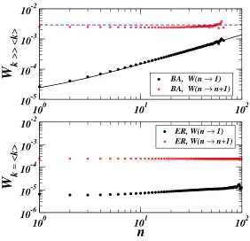
FIG. 5: Probability of winning and loosing (only the term causing an increase of the number of

words) for BA and ER models. Both with N _{= 5000 nodes and}k_{≃200 (for a BA with h}k_{i= 10)}

and k_{≃70 (for a ER withh}k_{i= 50). Data were obtained averaging over several runs (3}.₁₀4_{) the}

probability of successful or unsuccessful interactions after t_{= 5}.₁₀5 _{time-steps from the beginning}

of the process. In fact, the time has also in this case only a parametric influence on the observed

curves.

where the average inventory size_hn_itcomes from the mean-field hypothesis for the

neighbor-ing sites of a node playneighbor-ing as speaker, that is actually correct in all small-world topologies,

and pk and qk are the probabilities of playing as speaker and as hearer respectively. The

index r inWr

k is used to indicate that these transition rate are correct in the reorganization

region. The inventory size may increase only when the agent plays as hearer, i.e.

Wkr(n →n+ 1|t)≃qk

1₋ n

C(t)

. (4)

In order to verify the above expressions for some specific cases, we have computed

nu-merically the quantities _Wr

k(n →n+ 1|t) andWkr(n →1|t), in the case of a BA network of

N = 5_·103 _{nodes and hki= 10 (top panel in Fig. 5) and for an ER model with N = 5·10}3

nodes and _hk_i= 50 (bottom panel in Fig. 5).

For heterogeneous networks, the numerical _Wr

the quantity with n, in agreement with Eq. 3, while the approximately constant behavior

of _Wr

k(n→n+ 1|t) with n can be fitted with an expression of the form Eq. 4 only for very

small values of n/C(t). On the other hand, Fig. 5 (bottom) points out that in the case

of homogeneous networks, in which all nodes have approximately the same behavior, both

quantities are almost independent of n. The different behaviors of the transition rates are

responsible of the different shape of the probability distribution _Pn(k_|t).

B. Transition rates during the convergence process

When the convergence process begins, the temporal behavior of all global quantities

accelerates, and the expression of the success probability changes considerably. In all

small-world topologies, the convergence is reached by means of a sort of cascade process, triggered

by a symmetry breaking event in the space of the states (words, etc.) [7]. The state

involved in the symmetry breaking starts to win, becoming more and more popular among

the inventories. At the end of the process, when the global consensus is reached, this is the

only surviving state.

According to this analysis, as the system is close to the convergence, most of the successful

interactions involves the most popular state, while positive negotiations involving different

states rapidly disappear. The statistical behavior of the quantity |S_n∩_SH| depends now only

on the properties of the most popular word. The average size of the intersection set _|S_∩H_|

is well expressed by the probability αk(t) of finding the most popular state (or word) in

both the inventories. During the convergence process, αk(t) is close to one. With this

approximation we are neglecting the successful interactions due to less popular states, that

we will show to have an effect for the dynamics on the complete graph (see section V C).

According with this argument, the transition rates assume the following form,

Wkc(n→1|t)≃pk

αk(t)

n +qk

αk(t)

hn_it

, (5)

Wc

k(n →n+ 1|t)≃qk

1₋ αk(t)

hn_it

, (6)

where the index c is used to distinguish the expression of the transition rates during the

C. Validation of the adiabatic approximation

In both the reorganization and the convergence regions, the validity of the adiabatic

approximation can be proved computing the characteristic relaxation time of the

non-equilibrium process described by the master equation in Eq. 2 with transition rates of Eqs. 3-4

or Eqs. 5-6. Given the (continuous, for simplicity) master equation ∂_tP(t) =₋W_P(t), the

relaxation timeτ is defined as the inverse of the real part of the smallest non-zero eigenvalue

λ1 of the transition matrixW. The explicit diagonalization of the Markov transition matrix

for a finite system may be demanding, but the order of magnitude of τ is easy to compute.

We first note thatW =pkW¯ in both cases.

In the reorganization region, when C(t) _≫ 1, the real parts of the eigenvalues of ¯W are

O(k/_hk_i), thusλ1 _∝qk, and the time necessary to reach the stationary state isτ ∼ O(1/qk).

The argument holds even close to the consensus state, where C(t), _hn_it, and αk(t) are of

order 1, since the smallest non-zero eigenvalue is still _∝ qk. Note that, in all complex

net-works qk > 1/N, thus τ < N. The time-dependent quantities involved in the expressions

of the transition rates, such as _hn_it and C(t) and αk(t), vary on a slower timescale (the

characteristic timescale of the global system ist/N), justifying the adiabatic approximation.

D. General expression of the adiabatic solution in the two dynamical regions

Mathematically, the adiabatic approximation consists in setting to zero the temporal

derivative of the inventory size distribution, and looking at the stationary solution _Pn(k|t),

with parametric dependence on the time, that we call adiabatic solution. We compute

the general adiabatic solution of the master equation in the two regions, while the most

interesting cases are reported separately in the next section.

Let us first consider a general complex network in the reorganization region. Plugging

the expressions of the transition rates_Wr

k(n→n+ 1|t) andWkr(n →1|t) into the stationary

form of the master equation (Eq. 2), we get the following recursion relation,

Pn(k|t) =

qk

h

1_−Cn−_(t1₎i

qk

h

1₋ n C(t)

i

+qk_Cn_(t) +pkh_Cn₍i_tt₎

Then, introducing qk =kpk/hki =b(k)pk and Eq. 7 can be rewritten as

Pn(k|t) =

b(k)[1₋ n_C−_(t1₎]

b(k) + hnit

C(t)

Pn−1(k|t). (8)

Since n−1

C(t) ≪1, we can write 1−

n−1

C(t) ≃e

−n−1

C(t), thus solving the recurrence relation,

Pn(k|t)≃s(k, t)n−1e−

n(n₋1)

2C(t) P

1(k|t) , (9)

withs(k, t) = b(k)/b(k) + hnit

C(t)

. The normalization relation gives_P1(k|t). The controlling

parameter of the curve is s(k, t), that allows to tune the decay of the distribution between

an exponential and a Gaussian-like tail. A change of variable s(k, t) = 1 ₋ǫ(k, t) (with

ǫ(k, t) = hnit

b(k)C(t)) makes evident thats(k, t)

n

≈e−ǫ(k,t)n_{, therefore the curve has the behavior}

Pn(k|t)∝e−ǫ(k,t)n−

n(n₋1)

2C(t) . (10)

The linear term dominates when _hn_{it ≫} b(k), i.e. in homogeneous topologies, while the

quadratic term governs the shape of the distribution for the high-degree nodes in

heteroge-neous networks (_hn_it≪b(k)). This result is very interesting since it shows that heterogeneity

is a necessary condition for agents to show a super-exponential decay in the inventory size

distribution.

When we are in the convergence region, on the other hand, to get the form of the memory

size distribution we must insert the Eqs. 5-6 into the stationary version of Eq. 2,

∂_Pn(k|t)

∂t = 0 =qk

1₋ αk(t)

hn_it

Pn−1(k|t)−qk

1₋ αk(t)

hn_it

Pn(k|t)

−

pk

αk(t)

n +qk

αk(t)

hn_it

Pn(k|t).

(11)

We get the following recursive relation,

Pn(k|t) =

"

1₋ αk(t)

hnit 1 + αk(t)

b(k) 1

n

#

Pn−1(k|t) , (12)

in which b(k) =k/_hk_i. The general solution is of the form

Pn(k|t)∝n−

αk(t)

b(k) _e−

αk(t)

hnit n , (13)

evidence of power-law behaviors on complex networks. This can be explained looking at the

terms of Eq. 13. In homogeneous networks, the power-law has exponent close to 1 (since both

αk(t) and b(k) are of order 1), but the cut-off imposed by the exponential distribution sets

in at very low n, preventing the underlying power-law to be observed. The same argument

holds for low-degree nodes in heterogeneous networks, but high-degree nodes should present

sufficiently large inventories to see the power-law. However, in this case b(k)_≫ 1, thus the

exponent of the power-law is too small to be observed.

The only case in which we are able to observe a power-law inventory size distribution is that

of the complete graph, that presents some peculiarities and will be discussed separately in

the next section.

V. ADIABATIC SOLUTION FOR SOME INTERESTING CASES

In this section, we study more in detail the effects of the topology on the adiabatic

solution of the master equation making explicit calculations in three interesting cases: in

the reorganization region, we consider the activity statistics of generic nodes in homogeneous

random graphs and of hubs in heterogeneous scale-free networks; in the convergence region,

we focus on the purely mean-field behavior of agents placed on a complete graph.

A. The case of homogeneous networks

As revealed by simulations reported in Fig. 5 (bottom) the transition rates for

homoge-neous networks in the reorganization region are almost independent of the number of states

in the inventory. In homogeneous networks qk ≃ b(k)pk, with b(k) ≃ O(1), and the nodes

are in general equivalent, thus the number of states is approximately the same for every

node, i.e. n _{≃ h}n_it. The approximated expressions of the transition rates for a node of

typical degree k =_hk_i are

Wkr(n→1|t)≈pkhnit(1 +b(k))/C(t)≈2pkhnit/C(t) (14)

Wkr(n→n+ 1|t)≈b(k)pk

1₋ hnit

C(t)

Such approximations are in agreement with the data reported in Fig. 5-bottom.

The adiabatic condition for the master equation becomes

0 = _Pn−1(hki|t)− Pn(hki|t)− hnit_C2_(t)Pn(hki|t) n >1

0 = P∞

j=2 C2(t)hnitPj(hki|t)− P1(hki|t). (16)

The solution by recursion is very simple,

Pn(hki|t)≈(1−θ)θn−1 , θ =

1 1 + 2hnit

C(t)

. (17)

Using the expansion of logarithm log(1₋ǫ)_{≃ −}ǫ, withǫ= 1₋θ _≃2_hn_it/C(t), the previous

formula gives the following exponential decay for the distribution of the number of states,

Pn(hki|t)≃

2_hn_it

C(t)e

−2hnit

C(t)n . (18)

The exponential decay is in agreement with the numerical data. Knowing the complete

form of the distribution (i.e. with the correct normalization prefactor), we can also roughly

estimate _hn_it and C(t), at fixed timet, from a self-consistent relation for_hn_it, From Eq. 18,

we compute the approximate average value of _hn_it, i.e.

hn_it≈

Z ∞

1

n_Pn(hki|t)dn , (19)

and we get the self-consistent expression

hn_it≃

C(t)

2_hn_it

1 + 2hnit

C(t)

e−2h

nit

C(t) _{. (20)}

Now, introducing in Eq. 20 the numerical value of_hn_it/C(t), it is possible to verify that the

orders of magnitude of both _hn_{it ∼ O}(10) and C(t) _{∼ O}(102_{) are in agreement with their}

numerical estimates.

B. High-degree nodes in heterogeneous networks

Now we pass to describe the dynamics of the hubs in heterogeneous networks in the

reorganization region of the system. In a direct Naming Game, a hub is preferentially

chosen as hearer, by a factor b(k) =k/_hk_{i ≫} 1, then in the transition rates we can neglect

the terms associated with the speaker. We consider the following approximated expressions

Wkr(n→1|t)≃qk

n

C(t) , (21)

Wr(n_→n+ 1_|t)_≃q

1₋ n

in which the last approximation is justified by the fact that, in general,n/C(t)_≪1. Inserting

realistic values of qk and C(t), the Eqs. 21-22 are in agreement with the behaviors coming

from the fit of the corresponding curve in Fig. 5 (top).

We can easily compute the adiabatic solution _Pn(k|t) from Eq. 2

0 =qkPn−1(k|t)−

qk+qk

n

C(t)

Pn(k|t) , (23)

and we find recursively

Pn(k|t) = _CC_(t)+(t)_nPn−1|t(k) = C(t)

2

(C(t)+n)(C(t)+n−1)Pn−2(k|t) (24)

≈ C(Γ(t)nC−(1tΓ()+Cn(+1)t)+2)P1(k|t) . (25)

Now, from the closure relation P∞

n=1Pn(k|t) = 1 we get the expression of P1(k|t), and the final form for_Pn(k|t) becomes

Pn(k|t) =

C(t)n−1

Γ(C(t) +n+ 1)C(t)

C(t)+1

e−C(t)

Γ(C(t) + 1) γ(C(t) + 1, C(t))

, (26)

where γ(a, x) is the lower incomplete Gamma function. The functional form of the

sta-tionary distribution is complicated, but exploiting Stirling approximations for Gamma

functions we can easily write it into a much simpler form. Indeed, using the expression

Γ(x)_≈√2πe−x_xx−1/2 _{and the representation via Kummer hypergeometric functions for the}

incomplete Gamma function γ(a, x), we find that

lim

x→+∞

Γ(x+ 1)

γ(x+ 1, x) =const≃2, (27)

and this value is correct in the range of x=C(t)_≫1. Finally, using the asymptotic series

expansion of Γ(x+n+ 1) for large x, we get an expression that can be formally written as

Γ(x+n+ 1)_≈√2πe−xxx+n+1/2_×

O(1) +Q[_O((n+ 1)2)]x−1+Q[_O((n+ 1)4)]x−2+. . . , (28)

in which Q[_O((n+ 1)l_{)] is a polynomial in (n+ 1) of maximum degree l. Now, we can do}

the resummation of the series keeping at each order k in x only the highest term in the

polynomial in (n+ 1), whose coefficient is 2−k_/k!,

Γ(x+n+ 1)_≈√2πe−xxx+n+1/2

∞

X

k=0

x−k(n+ 1)2k

k!2k =

√

Putting together all the ingredients, we find that a good approximation of the distribution

of the number of words is given by (the half-Normal distribution)

Pn(k|t)≃

s

2

πC(t)e

−(n+1)2

2C(t) _{. (30)}

Fitting numerical results in Fig. 5 (top) with this expression provides values for C(t) _∼

O(102_{), showing that, as expected, on the BA model C(t)< N}

d(t)∼ O(102÷103).

C. Power-laws on the complete graph

The last interesting case consists in studying the inventory size distribution for agents on

the complete graph. In the reorganization region, the mean-field dynamics is characterized

by a large fraction of agents with _O(√N) states in their inventories and another smaller

fraction with exponentially distributed inventory sizes. The existence of a peak at _O(√N)

comes from the initial accumulation process (see Ref. [7]), while the exponential part of the

distribution is produced during the following reorganization regime. Since the most of the

agents have _O(√N) states and the intersection between inventories is close to zero, we can

write the following transition rates

Wkr(n→1|t)≈

2 N

1

√

N (31)

Wr

k(n →n+ 1|t)≈

1 N

1_{− √}1 N

(32)

With the usual recurrence relation we compute the following adiabatic solution,

Pn(k|t)∝f(t)δ(n− √

N) + (1₋f(t))e−√2Nn , (33)

with f(t) is the fraction of agents around √N that tends to zero the convergence

The interesting region is however the last one, during the convergence process, in which

the inventory size distribution of the mean-field system develops a power-law structure. In

Eq. 13, we have shown that the expected distribution in the convergence region presents a

power-law, that in the particular case of the complete graph should have an exponent close

to 1 (since αk(t)≃ 1). Nonetheless, Fig. 4 reveals that the slope −1 is correct only at the

mixed distribution emerging in the reorganization region, we explain how the alteration of

the power-law is due to the superposition of an exponential distribution.

During the convergence process, the agents having access to the most popular state behaves

following the transition rates in Eqs. 5-6 and their activity is at the origin of the power-law

in _Pn(k|t). The other agents, that have no access to the most popular state maintain an

inventory of size about√N and fall to 1 if they get a successful interaction. In other words,

they keep on playing as in the reorganization region, generating an exponential distribution

of the inventory sizes. Even if the fraction of these agents decreases in time, the superposition

of the exponential on the power-law has the immediate effect of increasing the slope of the

power-law at low n.

In summary, we have provided an explanation of the behavior of the activity patterns of

the Naming Game on the complete graph, pointing out some fundamental differences with

respect to generic complex networks.

VI. CONCLUSIONS

We have studied the microscopic activity patterns in a population of agents playing the

Naming Game proposed in Ref. [7]. Previous work pointed out that the non-equilibrium

dynamical behavior of the model presents very different features depending on the underlying

topological properties of the system[7, 9, 10]. The analysis, however, were focused on the

behavior of global quantities, while in the present work we have investigated the microscopic

activity patterns of single agents. Indeed, by means of numerical simulations and analytical

approaches, we have shown that the negotiation process between agents is at the origin of

a very rich internal activity in terms of variations of the inventory size. More precisely, our

analysis has focused on the instantaneous activity statistics described by the distribution

Pn(k|t) that an agent of degree k has an inventory of size n at time t. We have been able

to explain its behavior in function of both the global temporal evolution and the underlying

topology of the system.

Apart from an initial transient, the dynamics of the Naming Game can be split in two

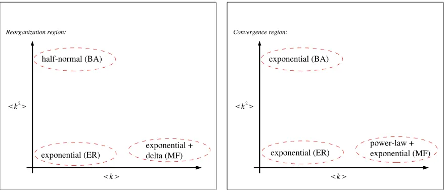
temporal regions, namely the reorganization part and the convergence part. Fig. 6

sum-marizes our findings, showing the microscopic activity statistics in function of the first two

FIG. 6: Phase plane like pictures in which the topological affects on the microscopic activity of the

Naming Game are summarized. Left figure displays the situation in the reorganization region, in

which the major effect is due to the increase of the degree fluctuations (the memory size distribution

passes from an exponential to a half-normal distribution. In the right panel, we show the same

picture for the convergence region, in which the final cascade process of convergence porduces a

power-law like memory size distribution. Such a distribution is however visible only in the purely

mean-field case, while on generic complex networks is covered up by exponential terms. The region

at both large average degree and fluctuations is difficult to be explored, but should correspond to

mixed distributions in which all previously classified behaviors may be observed.

networks affecting the dynamics of the _Pn(k|t). In the left panel of Fig. 6 we sketch the

relation between topology and single agent activity in the reorganization region. Increasing

the heterogeneity of the nodes the_Pn(k_|t) shifts from an exponential to a super-exponential

(half normal) regime. Increasing _hk_i while preserving the homogeneity of the nodes, on

the other hand, leads to a superposition of an exponential and a delta at √N. A class of

distributions mixing up all these features is observed for networks with diverging average

degree and fluctuations (top-right corner of the plane). A similar summary describes the

effect of the topology in the convergence region (Fig. 6, right panel): increasing the average

degree, the distribution moves from exponential to a superposition of an exponential and

a power-law, while larger fluctuations destroy the power-law leaving only an exponential

distribution.

properties of processes taking place on them is the object of a vast interest in statistical

physics community. However, only global properties are usually considered. Here, we have

focused on the internal dynamics of single agents, and we have found results providing

ex-planation for the strong converging property of the corresponding global dynamics. Indeed,

one of the most interesting aspects of the Naming Game is exactly that the number of states

an agent can store is not fixed a priori and the update rule involves a memory-based

nego-tiation process. This is a relevant difference with most of the well known models in various

fields of statistical mechanics or opinion dynamics, such as the voter or the Axelrod models,

and we have investigated its deep consequences on the global behavior of the system.

A last remark concerns the comparison with usual statistical mechanics models. In this

regard, it is useful to shift our perspective and look at the waiting time between successive

decision events. In the present case, a decision event corresponds to a successful interaction,

so that the waiting time is directly proportional to the inventory size. In the non-equilibrium

glauber dynamics, for instance, a decision event is commonly associated to a spin flip. The

corresponding waiting time is exponentially distributed during the dynamics (poissonian

dy-namics), but close to the convergence (to the ferromagnetic state) the waiting time between

two flips may diverge, and its distribution assumes a power-law shape. As we have shown, a

similar behavior is observed and proved for the inventory size distribution in the mean-field

Naming Game. The inventory size statistics in the Naming Game can be thus compared to

waiting time statistics in other models. According to our analysis, it should be interesting

to further investigate the relation between topology and individual waiting time statistics

in other models of collective dynamics presenting similar non-poissonian individual activity.

Acknowledgments

The authors thank A. Barrat and V. Loreto for many useful discussions. L.D. is partially

supported by the EU under contract 001907 (DELIS). A.B. is partially supported by the

EU under contract IST-1940 (ECAgents).

[2] L.Steels, Proceedings of PPSM VI in Lecture Notes in Computer Science, Springer-Verlag,

Berlin (Germany), 2000.

[3] R. Lass, Historical Linguistics and Language Change, Cambridge University Press

(Cam-bridge), 1997. T. Briscoe, Linguistic evolution through language acquisition: formal and

com-putational models, Cambridge University Press (Cambridge), 1999. J. Hurford, C. Knight,

and M. Studdert-Kennedy (eds.), Approaches to the Evolution of Human Language,

Cam-bridge University Press (CamCam-bridge), 1999.

[4] L. Steels, Evolution of Communication 1, 1-34 (1997).

[5] S. Kirby, Artificial Life8, 185-215 (2002).

[6] L. Steels, Artificial Life,2(3), 319-332 (1995).

[7] A. Baronchelli, M. Felici, E. Caglioti, V. Loreto and L. Steels,preprint, arxiv:physics/0509075

(2005).

[8] P. L. Krapivsky,Phys. Rev. A 45, 1067 (1992).

[9] L. Dall’Asta, A. Baronchelli, A. Barrat, and V. Loreto, preprint(2006).

[10] L. Dall’Asta, A. Baronchelli, A. Barrat, and V. Loreto,Europhys. Lett.73(6), 969-975 (2006).

[11] S. N. Dorogovtsev and J. F. F. Mendes, Evolution of Networks: from biological nets to the

Internet and WWW (Oxford University Press, Oxford 2003).

[12] R. Pastor-Satorras and A. Vespignani, Evolution and structure of the Internet: A statistical

physics approach (Cambridge University Press, Cambridge, 2004).

[13] A. Baronchelli, L. Dall’Asta, A. Barrat, and V. Loreto, Phys. Rev. E 73, 015102(R) (2006).

[14] C. CastellanoAIP Conf. Proc. 779, 114 (2005).

[15] S. Franz and F. Ritort, J. Phys. A: Math. Gen.30, L359 (1997).

[16] F. Ritort and P. Sollich, Adv. Phys. 52, 219 (2003).

[17] W. Feller, An Introduction to Probability Theory and Its Applications, Volume 1 John Wiley

& Sons (New York), 1968.

[18] We call ”learning process” the dynamics of acquisition and deletion of states from the point of

view of a single agent. The terminology is reminiscent of the original purposes of the Naming