Parameter estimation for the stochastic SIS epidemic model

Parameter Estimation for the Stochastic SIS

Epidemic Model

Jiafeng Pan, Alison Gray, David Greenhalgh, Xuerong Mao

Department of Mathematics and Statistics,

University of Strathclyde, Glasgow G1 1XH, U.K.

Abstract

In this paper we estimate the parameters in the stochastic SIS epidemic model by using pseudo-maximum likelihood estimation (pseudo-MLE) and least squares estimation. We obtain the point estimators and 100(1₋α)% confidence intervals as

well as 100(1₋α)% joint confidence regions by applying least squares techniques.

The pseudo-MLEs have almost the same form as the least squares case. We also obtain the exact as well as the asymptotic 100(1₋α)% joint confidence regions for

the pseudo-MLEs. Computer simulations are performed to illustrate our theory.

Key words: Stochastic SIS epidemic model, pseudo-maximum likelihood estima-tion, least squares estimaestima-tion, confidence interval, confidence region, asymptotic estimator, logistic equations.

1

Introduction

In general parameter estimation in stochastic differential equations (SDEs) is a non-trivial problem [2, 9]. Many SDEs are non-linear, making simpler approaches to estimation im-possible to implement. Young [27] reviews parameter estimation methods for continuous time models. Nielsen et al. [21] updates this to include newer methods for discretely observed SDEs. Timmer [26] discusses the relation between Maximum Likelihood Esti-mators (MLEs) and quasi-MLEs and compares the quasi-MLE approach with the ∆t=δt

approach in simulations. Kristensen et al. [11] considers the stochastic ’grey box’ model and presents the approximate MLE approach based on normal approximation and use of the extended Kalman filter and a software package CTSM. Bishwal [2] discusses the asymptotic properties of MLEs and Bayes estimators of real valued drift parameters in SDEs. Parameter estimation for stochastic delay differential equations (SDDEs) in par-ticular has been studied for the last ten years, see e.g. [7, 12, 13, 14, 23, 24, 25].

confidence into account. Also, we investigate the factors which influence the width of the confidence intervals and the area of the confidence regions both analytically and in our simulation examples.

The well-known SIS model is one of the simplest epidemic models and is often used to model diseases for which there is no immunity, including gonorrhea [8], pneumococcus [15, 17] and tuberculosis.

In our previous paper [6], we derived an Itˆo SDE SIS model from the deterministic one

dS(t) = [µN₋βS(t)I(t) +γI(t)₋µS(t)]dt₋σS(t)I(t)dB(t),

dI(t) = [βS(t)I(t)₋(µ+γ)I(t)]dt+σS(t)I(t)dB(t) (1.1)

with initial values S0 +I0 = N, where S0 and I0 are initial numbers of susceptible and infected individuals in a population of sizeN. S(t) andI(t) are the numbers of susceptible and infected individuals at time t and B(t) is a scalar Brownian motion. This model has parameters β, γ, µ and new parameter σ. Here µ is the per capita death rate, and γ

is the rate at which infected individuals become cured, so 1/γ is the average infectious period. The parameter β is the disease transmission coefficient, so that β =λ/N where

λ is the per capita disease contact rate. The parameter λ is the average number of adequate contacts of an infective per day. An adequate contact is one which is sufficient for the transmission of an infection if the contact is between a susceptible and an infected individual. Regarding the parameter σ, σ2_{dt quantifies the size of the variance of the}

number of potentially infectious contacts that a single infected individual makes with another individual in the small time interval [t, t+dt).

As S(t) +I(t) =N, it is sufficient to study the SDE for I(t)

dI(t) =I(t)[βN ₋µ₋γ ₋βI(t)]dt+σ(N ₋I(t))dB(t) (1.2)

with initial value I(0) = I0 _∈(0, N), and in the rest of the paper we will concentrate on this SDE only.

The organization of this paper is as follows: In section 2 we apply the least squares estimation approach to our problem and obtain the point estimators, interval estimators and confidence regions for the model parameters β, η = µ+γ and σ2_{. We consider the}

cases of parameter estimation for both one sample of data and multiple samples. We also investigate the factors which influence the width of the confidence intervals and the areas of the confidence regions. Simulation examples are given to illustrate our theory. In section 3 we discuss the pseudo-MLE method. We obtain the maximum likelihood estimators and exact and approximate confidence regions, and again consider the case of multiple samples. Also we compare the pseudo-MLEs with the least squares estimators both analytically and in our simulation examples. In section 4 we summarise the findings in the paper and indicate further ongoing work to be reported.

2

Least Squares Estimation

model. Then the regression theory can immediately be applied to estimate the model parameters. In this section point estimators, 100(1₋α)% confidence intervals as well as 100(1₋α)% joint confidence regions will be obtained for our model parameters. Simulation examples will be given to illustrate our theory.

2.1

Regression Model

Let_{Ik}nk=0be observations from process (1.2). Given a stepsize ∆tand settingI0 =I(0),

the EM scheme produces the following discretization over small intervals [k∆t,(k+ 1)∆t]

Ik+1−Ik =Ik(βN −µ−γ−βIk)∆t+σ(N −Ik)Ik∆Wk, (2.1)

where ∆Wk =Wk+1−Wk.

Equation (2.1) can be rewritten as

yk+1 =ηuk+1+c+σZk+1, (2.2)

where yk+1 = I

k+1−Ik

Ik(N−Ik) √

∆t, η =µ+γ, uk+1 =−

√

∆t N−Ik,c=

√

∆tβ and Zk+1 ∼N(0,1). We

can get the observations (yi, ui)ni=1if data points{Ik}nk=0and stepsize ∆tare provided. We

then write the model as yi =ηui+c+εi (i= 1,2, ..., n), where εi ∼N(0, σ). This looks

like a simple linear regression model but with the difference that y = (y1, y2, ..., yn) is a

random variable instead of a response variable which is conditional onu= (u1, u2, ..., un).

However we still can use the regression theory to estimate η and β since estimation is based on the least squares method, i.e. to minimize Pn

i=1(yi−ηui−c)2, which is not

affected by whether y is a random variable or not.

Rawlings (1998) [22] discusses multiple linear regression in the general matrix form

Y=Xθ+ε, (2.3)

where

Y =



   

y1 y2

...

yn



   

, X =



   

1 x11 x12 _{· · ·} x1p

1 x21 x22 _{· · ·} x2p

... ... ... ... ... 1 xn1 xn2 · · · xnp



   

, θ =



   

θ0 θ1

...

θp



   

, ε =



   

ε1 ε2

...

εn



   

.

The calculations work equally well for (2.2), which can be written in the matrix form (2.3), where Y and ε remain the same whileX and θ become

X =



   

√

∆t u1

√

∆t u2

.. . ...

√

∆t un



   

, θ=

β η

2.2

Point Estimators

We use the formulae in the multiple linear regression theory to derive the estimators for

η and β as

_ˆ

β

ˆ

η

= ˆθ= (XTX)−1_(XT_Y)

= 1

n∆tP

u2

k−∆t(

P

uk)2

√

∆tP

u2

k

P

yk−

√

∆tP

ukPukyk

n∆tP

ukyk−∆tPukPyk

.

(2.4)

HereP

represents Pn−1

k=0 as does the

P

below. Then we have point estimators as

ˆ β = P u2 k P

yk−PukPukyk

n√∆tP

u2

k−

√

∆t(P

uk)2

(2.5)

and

ˆ

η = n

P

ukyk−PukPyk

nP

u2

k−(

P

uk)2

, (2.6)

which are equal to

ˆ

β =

P 1

(N−Ik)2

P Ik₊₁₋Ik

Ik(N₋Ik) −

P 1

N−Ik

P Ik₊₁₋Ik

(N−Ik)2Ik

nP _∆t

(N−Ik)2 −

P √_∆t

N−Ik

2 (2.7)

and

ˆ

η =

P Ik+1−Ik

Ik(N−Ik)

P ₁

N−Ik −n

P Ik+1−Ik

(N−Ik)2Ik

nP ∆t

(N−Ik)2 −

P √∆t

N−Ik

2 . (2.8)

We consider a time interval of total lengthT divided intonsubintervals each of length ∆t so n∆t = T. Hence as n _{→ ∞} and ∆t _→ 0 with n∆t = T, the sums approach the integrals, i.e.

n−1

X

k=0

∆t

(N ₋Ik)2 →

Z T

0

1 (N ₋I)2 dt

n−1

X

k=0

Ik+1−Ik

Ik(N−Ik) →

Z I(T)

I(0)

1

I(N ₋I)dI etc.

Hence we have that as n_{→ ∞}, ˆβ and ˆη tend to

ˆ

β =

RT

0 1

(N−I(t))2 dt·

RI(T)

I(0) 1

(N−I)IdI −

RT

0 1

N−I(t)dt·

RI(T)

I(0) 1 (N−I)2IdI

T RT

0 1

(N−I(t))2 dt−

RT

0 1

N−I(t)dt

2

and

ˆ

η=

RI(T)

I(0) 1

(N−I)IdI·

RT

0 1

N−I(t)dt−T

RI(T)

I(0) 1 (N−I)2IdI

T RT

0 1

(N−I(t))2 dt−

RT

0 1

N−I(t)dt

2.3

Variance of Estimated Parameters

Confidence interval estimators of parameters give more information than simple point estimators. To obtain interval estimators for the parametersβ andη, we need to calculate the variance of θˆusing the formula

var(θˆ) = (XTX)−1_σ2_{, (2.9)}

where σ2 _{can be estimated using the residual mean square}

ˆ

σ2 = (Y−Xθˆ)

T_(Y−Xθˆ₎

n₋p , (2.10)

where p is the number of parameters and is 2 in this case. Equation (2.10) can be simplified as

ˆ

σ2 = Y

T_Y−YT_Xθˆ

n₋2 (2.11)

if we substitute ˆθ = (XTX)−1_(XT_{Y) in (2.10).}

Then equation (2.11) can be written as

ˆ

σ2 = 1

n₋2

X

y_k2₋√∆tXyk

ˆ

β₋ Xykuk

ˆ

η

!

. (2.12)

Substituting (2.4) in (2.12) we get ˆ

σ2 ₌

nP

y2

k

P

u2

k−

P

y2

k(

P

uk)2−Pu2k(

P

yk)2−n(Pykuk)2+ 2PukPykPykuk

(n₋2) nP

u2

k−(

P

uk)2

,

(2.13) which is

1

n

nP ∆t

(N−Ik)2 −∆t

P 1

N−Ik

2

nX (Ik+1−Ik) 2

Ik2(N −Ik)2

X 1

(N ₋Ik)2 −

X (I_k+1−I_k)2

Ik2(N −Ik)2

X 1

N ₋Ik

2

−X 1

(N₋Ik)2

X I_k+1−I_k

Ik(N −Ik)

2

−n

X I_k+1−I_k

Ik(N −Ik)2

2

+ 2X 1

N ₋Ik

X I_k+1−I_k

Ik(N −Ik)

X I_k+1−I_k

Ik(N −Ik)2

!

.

(2.14)

Theorem 2.1 The estimator σˆ2 _{in (2.12) is an asymptotically unbiased estimator for σ}2 in (2.2), i.e.

ˆ

σ_n2 _→σ2 a.s.

Proof.

ˆ

σ2 = RSS

n₋p =

1

n₋2

X

(yk−yˆk)2, (2.15)

where RSS is the sum of squares of residuals for model (2.2) and p is the number of parameters to be estimated.

After substituting for ˆβ and ˆη using (2.5) and (2.6)

yk−yˆk=yk

−

P

iu2i

P

iyi−

P

iui

P

iuiyi

∆

− (n

P

iuiyi−

P

iui

P

iyi)uk

∆ ,

where ∆ =nP

iu2i −(

P

iui)2 and Pi represents

Pn−1

i=0 here and throughout the rest of

the paper. Since yk =β

√

∆t+ηuk+σZk,

yk−yˆk =β

√

∆t+ηuk+σZk

−

P

iu2i

P

i(β

√

∆t+ηui+σZi)−PiuiPiui(β

√

∆t+ηui+σZi)

∆

−[n

P

iui(β

√

∆t+ηui+σZi)−P_iuiP_i(β

√

∆t+ηui+σZi)]uk

∆ .

Therefore ˆσ2 _{can be simplified as}

σ2 n₋2

X

Zk−

uknPiuiZi−ukPiZiPiui+Piui2PiZi−PiuiPiuiZi

∆

!2

,

which is equal to

σ2 n₋2

X

Zk2+

nukP_iuiZi−ukP_iZiP_iui

∆

!2

+

P

iui2

P

iZi−

P

iui

P

iuiZi

∆

!2

−2Zk

nukP_iuiZi−ukP_iZiP_iui

∆ −2Zk

P

iui2

P

iZi−

P

iui

P

iuiZi

∆

+ 2(ukn

P

iuiZi−uk

P

iZi

P

iui) (

P

iui2

P

iZi −

P

iui

P

iuiZi)

∆2

!

.

This can be simplified as

σ2 n₋2

X

Zk2+

1 ∆2

X

uk2

X

Zk

2_X

uk

2

−n2XukZk

2_X

uk2

−nXuk2

2_X

Zk

2

+nXukZk

2_X

uk

2

−2Xuk

3_X

Zk

X

ukZk+ 2n

X

uk

X

ukZk

X

uk2

X

Zk

!

which equals

σ2 n₋2

X

Zk2+ −

n(P

ukZk)2−Puk2(PZk)2+ 2PukPukZkPZk

nP

uk2−(Puk)2

!

.

This can be written as

σ2 n₋2

X

Zk2−A·

(P

ukZk)2

P

uk2 −

A_· (

P

Zk)2

n +B·

P

ukZk

pP

uk2

· P Zk √ n ! , (2.16) where

A= n

P

u2

k

nP

u2

k−(

P

uk)2

, B = 2_·

√ npP u2 k P uk nP u2

k−(

P

uk)2

.

Note that _P

Zk

√_n ∼N(0,1) and

P

ukZk

pP

u2

k

∼N(0,1),

sinceZk ∼N(0,1) and theZk are independent. Moreover (

P

Zk)2

n and

(P

ukZk)2

P

u2

k have mean

1 and variance v, where v can be worked out and is independent ofn (it is the variance of the square of a standard normal random variable).

Therefore

σ2

n₋2 −A· (P

ukZk)2

P

uk2 −

A_· (

P

Zk)2

n +B·

P

ukZk

pP

uk2

· P Zk √ n !

→0 a.s.

as n_{→ ∞}. Also Z2

k has mean 1 and variance v2 independent of n since Zk ∼N(0,1). Therefore

1

n

P

Z2

k →N(1,vn2) asn → ∞by the Central Limit Theorem.

Hence ˆσ2 _→σ2 _{with probability one asn → ∞as required. 2}

Using ˆσ2 _{to estimate σ}2 _{in (2.9) we have}

var(θˆ) =var

_ˆ β ˆ η = 1

n∆tP

u2

k−∆t(

P

uk)2

P

u2

k −

√

∆tP

uk

−√∆tP

uk n∆t

ˆ

σ2. (2.17)

2.4

Interval Estimation

The distribution of the parameter estimators ˆβand ˆηifσ2 _{is known is exactly multivariate}

(actually bivariate) normal by the least squares regression theory [22]. However we are estimating σ2 _{by ˆσ}2_{. Hence if the number of observations n is large, the approximate}

100(1₋α)% confidence intervals (CIs) for β and η respectively are

ˆ

β_±zα/2

q

var( ˆβ) =

P

u2

k

P

yk−PukPukyk

n√∆tP

u2

k−

√

∆t(P

uk)2

±zα/2

s

P

uk2σˆ2

n∆tP

u2

k−∆t(

P

uk)2

and

ˆ

η_±zα/2

p

var(ˆη) = n

P

ukyk−PukPyk

nP

u2

k−(

P

uk)2 ±

zα/2

s

n∆tσˆ2 n∆tP

u2

k−∆t(

P

uk)2

, (2.19)

where zα/2 is the upper α/2 value of the standard normal random variable, e.g. z0.025 =

1.96 for a 95% CI.

We notice that as n_{→ ∞}, the 100(1₋α)% CIs tend to

RT

0 1

(N−I(t))2 dt·

RI(T)

I(0) 1

(N−I)IdI−

RT

0 1

N−I(t)dt·

RI(T)

I(0) 1 (N−I)2IdI

T RT

0 1

(N−I(t))2 dt−

RT

0 1

N−I(t)dt

2

±zα/2

v u u u t RT 0 1

(N−I(t))2 dt·σ

2

TRT

0 1

(N−I(t))2 dt−

RT

0 1

N−I(t)dt

2

and

RI(T)

I(0) 1

(N−I)IdI·

RT

0 1

N−I(t)dt−T

RI(T)

I(0) 1 (N−I)2IdI

T RT

0 1

(N−I(t))2 dt−

RT

0 1

N−I(t)dt

2

±zα/2

v u u t

T σ2

T RT

0 1

(N−I(t))2 dt−

RT

0 1

N−I(t)dt

2,

respectively.

Theorem 2.2 The asymptotic widths of the CIs for both β and η, which are

2_×zα/2

v u u u t RT 0 1

(N−I(t))2 dt·σ 2

T RT

0 1

(N−I(t))2 dt−

RT

0 1

N−I(t)dt

2

and

2_×zα/2

v u u t

T σ2

T RT

0 1

(N−I(t))2 dt−

RT

0 1

N−I(t)dt

2,

are strictly decreasing as T increases.

Proof. Considering first the width of the CI for β,

RT

0 1 (N−I(t))2 dt TRT

0 1

(N−I(t))2 dt−

RT

0 1

N−I(t)dt

2 =

1

T ₋ (

RT

0 N₋1I(t)dt) 2

RT

0 (N₋1I(t))2dt

Then the derivative of the denominator is equal to

d dT





T −

RT

0 1

N−I(t)dt

2

RT

0 1 (N−I(t))2 dt



 

= 1₋ 2RT

0 1

N−I(t)dt 1

N−I(T)

RT

0 1

(N−I(t))2 dt−

1 (N−I(T))2

RT

0 1

N−I(t)dt

2

RT

0 1 (N−I(t))2 dt

2

=

RT

0 1

(N−I(t))2 dt− 1

N−I(T)

RT

0 1

N−I(t)dt

2

RT

0 1 (N−I(t))2 dt

2 ≥0.

Given a sample pathI(t) defined on the interval [0, T] with I(0)>0, we deduce that

I(T)_∈(0, N) [6]. The only way that the denominator of (2.20) is not strictly decreasing is if

Z T

0

1

(N₋I(t))2 dt= 1

N ₋I(T)

Z T

0

1

N ₋I(t)dt

on an interval [T, T +ε] for some ε >0. So if ∆T is small enough

(N ₋I(T + ∆T))

Z T+∆T

0

1

(N ₋I(t))2 dt=

Z T+∆T

0

1

N ₋I(t)dt (2.21)

and

(N₋I(T))

Z T

0

1

(N ₋I(t))2 dt=

Z T

0

1

N ₋I(t)dt. (2.22)

Subtracting (2.22) from (2.21) we have

[(N₋I(T + ∆T))₋(N ₋I(T))]

Z T+∆T

0

1

(N ₋I(t))2 dt

+ (N ₋I(T))

Z T+∆T

0

1

(N ₋I(t))2dt−

Z T

0

1

(N ₋I(t))2 dt

!

=

Z T+∆T

0

1

N ₋I(t)dt−

Z T

0

1

N ₋I(t)dt,

which is equal to

(₋I(T + ∆T) +I(T))

Z T

0

1

(N ₋I(t))2 dt+

∆T

(N ₋I(T))2 +o(∆T)

!

+ (N ₋I(T)) ∆T

(N ₋I(T))2 +o(∆T)

!

= ∆T

This equals

−I(T)(βN ₋η₋βI(T))∆T +σ(N ₋I(T))[B(T + ∆T)₋B(T)] +o(∆T)

Z T

0

1

(N ₋I(t))2 dt=o(∆T).

Dividing by √∆T we have

−I(T)

(βN ₋η₋βI(T))√∆T +σ(N ₋I(T))B(T + ∆_√T)−B(T) ∆T

=o(√∆T).

Letting the time step ∆T be very small and choosingε0 >0,_∃∆T0 _≤1 such that for ∆T <∆T0 the o(√∆T) term is between ₋ε0σI(T)(N ₋I(T))√∆T and +ε0σI(T)(N ₋ I(T))√∆T, hence must lie between ₋ε0σI(T)(N ₋I(T)) andε0σI(T)(N ₋I(T)).

Hence the term

B(T + ∆T)₋B(T)

√

∆T ∈ −

βN ₋η₋βI(T)

σ(N ₋I(T)) −ε0,−

βN ₋η₋βI(T)

σ(N ₋I(T)) +ε0

!

.

But B(T+∆T)−B(T)

√

∆T ∼ N(0,1) so the probability that it lies in the above interval tends to

zero as ε0 _→0. Hence

P

Z T

0

1

(N ₋I(t))2dt= 1

N ₋I(T)

Z

1

N ₋I(t)dt on [T, T +ε] for someε >0

!

= 0.

So the denominator of (2.20) is strictly increasing and the width of the CI for β is strictly decreasing in T. Similarly we can prove the case for η. 2

In the same way as for the simple linear SDE case, the asymptotic widths of the CIs here do not depend on the size of time step ∆t but only on the total time period T, and are decreasing as T increases.

2.5

Joint Confidence Region

We have obtained univariate CIs for each parameterβ andη in the last section. However individual CIs do not take into account the correlation among the parameters. Also, they do not reflect the overall degree of confidence. Joint confidence regions take both issues into account. So we will obtain a joint confidence region forβ and η in this section.

A 100(1₋α)% joint confidence region for the general regression model (2.3) is obtained from the following inequality [22]

(θ₋θˆ)T(XTX)(θ₋θˆ)_≤pσ2Fα,p,ν (2.23)

whereFα,p,ν is the value of theF-distribution with degrees of freedompand ν that leaves

Our case only involves two parameters so the 100(1₋α)% joint confidence region for

β and η can be written as

_ˆ

β

ˆ

η

−

β η

T

(var( ˆβ,ηˆ))−1

_ˆ

β

ˆ

η

−

β η

≤2Fα,2,n−2. (2.24)

After substituting (2.17) in (2.24), it can be easily calculated as

n∆tβˆ₋β2+ 2√∆tXuk( ˆβ−β)(ˆη−η) +

X

uk2(ˆη−η)2 ≤2ˆσ2Fα,2,n−2, (2.25)

where ˆβ and ˆη are known in (2.4). We compute that

4∆tXuk

2

−4n∆tXu2_k = 4∆t Xuk

2

−nXu2_k

!

. (2.26)

Defining the vectors in Rn

a= (1,1, ...,1) and b = (u1, u2, ..., un).

then _|a_|2_|b_|2 _{≥ |}a_·b_|2 as_|a_·b_|=_|a_||b_|cosθ, whereθ is the angle between aand b. Then we have _|a_|2 =n, _|b_|2 =P

u2

k and |a·b| = (

P

uk)2. So (2.26) is strictly negative since

the angle between a and b is not 0. Therefore the boundary of the 100(1₋α)% joint confidence region is an ellipsoid.

Example 2.5.1 Assume that the parameters are given by T = 1, I(0) = 10, β =

0.5, µ = 20, γ = 25, N = 100, and σ2 _{= 0.03 for the model (1.2). T = 1 is scaled} to represent one year and N = 100 represents 100 million people. We will use the same scaling for the rest of the examples.

We simulate I(t) using the above parameters by the EM method with a very small step size∆t= 0.001 and save theseI(t)as our true data set. Then we sample every 10th data point in the data set to obtain the sample for our parameter estimation, so n= 100

observations and ∆t= 0.01for our sample.

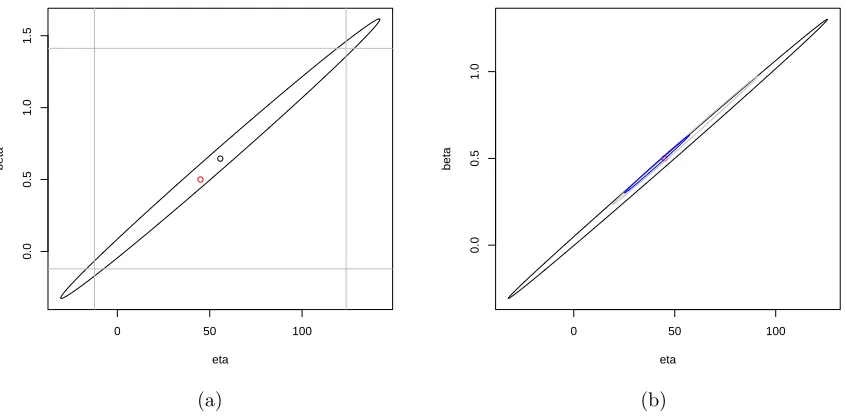
With the sample we obtained, with α = 0.05 we find the boundary of the 95% joint confidence region for β andη by using (2.25) and the univariate95%CIs for each of them by using (2.18) and (2.19), and also the point estimators by using (2.5) and (2.6), which are shown in Figure 1a. The ellipsoid in the figure represents the 95% joint confidence region while the grey lines represent the univariate CIs. We see that most of the ellipsoid lies in the square which represents the univariate CIs, but the area of the ellipsoid is much smaller than the square. It indicates the advantage of the joint confidence region that it drops out many of the extreme values in the univariate CIs and is more efficient. We see that the ellipsoid is centered at the point estimators of β and η. The red point which represents the true value of β= 0.5 and η= 45 lies in the ellipse.

Example 2.5.2 Assume that the parameters are given by I(0) = 10, β = 0.5, µ =

0 50 100

0.0

0.5

1.0

1.5

eta

beta

(a)

0 50 100

0.0

0.5

1.0

eta

beta

(b)

Figure 1: (a) is the 95% joint confidence region forβ and η obtained using the parameter values in Example 2.5.1 with T = 1. The ellipsoid in the figure represents the 95% joint confidence region, while the grey vertical and horizontal lines represent the univariate CIs for each of β and η. The black point marked in the figure is the point estimate for β and

η, and the red point represents the true values ofβ = 0.5 and η= 45; (b) is the 95% joint confidence region for β and η using the parameter values in Example 2.5.2, with T = 5 (black), T = 20 (grey) and T = 50 (blue). The red point represents the true value of

β = 0.5 and η= 45.

In order to see the influence of different interval lengthsT on the95%joint confidence region, we now vary the value of the interval length T as T = 5, T = 20 and T = 50 and use the same method as in Example 2.5.1 to simulate a data set for each T and sample from each of them. When we increase T we increase the number of observations n in proportion to T to keep ∆t fixed. We then obtain the three 95% joint confidence regions for the different values of T, which are shown in Figure 1b. We see that the area of the

95%joint confidence region becomes smaller with largerT (larger sequence of observations n). The red point which represents the true value of β = 0.5 and η = 45 lies in all the ellipses.

2.6

Estimation from Improved Regression Model with More

Data Sets

The CIs for bothβandηare dependent on the sample path. If more data sets are available, we can expand the original regression model to get better parameter estimation.

the regression model (2.2), so that Y,X,θ and ε become Y=                          y11 y12 .. .

y1n

y21 y22 ... y2n .. .

ym1 ym2

... ymn                         

, X=

                          √

∆t u11

√

∆t u12

.. . ...

√

∆t u1n

√

∆t u21

√

∆t u22

... ...

√

∆t u2n

.. . ...

√

∆t um1

√

∆t um2

... ...

√

∆t umn

                         

, θ =

β η

, ε=

                         ε11 ε12 .. .

ε1n

ε21 ε22 ... ε2n .. .

εm1 εm2

... εmn                          ,

using the same formula as in (2.4) we have

_ˆ

β

ˆ

η

= ˆθ = (XTX)−1_(XT_Y)

= 1

mn∆tP P

u2

ij −∆t(

P P

uij)2

√

∆tP P

u2

ij

P P

yij −

√

∆tP P

uijP Puijyij

mn∆tP P

uijyij −∆tP PuijP Pyij

,

(2.27)

where P P

=Pm

i=1

Pn−1

j=0 and similarly below.

In the same way, we can get

ˆ

σ2 = Y

T_Y−YT_Xθˆ

mn₋2

= 1

mn₋2

X X

y2

ij −

√

∆tX Xyij

ˆ

β₋ X Xyijuij

ˆ

η

!

= 1

(mn₋2) mn∆tP P

u2

ij −∆t(

P P

uij)2

· mn∆t

X X

y_ij2 X Xu2_ij

−∆tX Xy_k2X Xuij

2

−∆tX Xu2_ijX Xyij

2

−mn∆tX Xyijuij

2

+ 2∆tX Xuij

X X

yij

X X

yijuij

!

.

(2.28)

When proving ˆσ2 _{is an asymptotically unbiased estimator of σ}2_{, the procedure is}

similar to the one we used before. We use an equation similar to (2.15),

ˆ

σ2 = 1

mn₋2

X X

After almost identical working to that used before, we can simplify ˆσ2 _{as in (2.16), except}

that the P

now represents Pm

i=1

Pn−1

j=0 and the denominator under σ2 is mn−2. We

know that n_{→ ∞} implies mn_{→ ∞}.

So following almost the same procedure for the proof as before, we can prove that ˆ

σ2 _→σ2 _{with probability one as n→ ∞.}

Using formula (2.9) and ˆσ in (2.28) to estimate σ we have

var(θˆ) =var

_ˆ β ˆ η = 1

mn∆tP P

u2

ij −∆t(

P P

uij)2

P P

u2

ij −

√

∆tP P

uij

−√∆tP P

uijmn∆t

ˆ

σ2.

(2.29) If the number of observations is large, the 100(1₋α)% CIs for β and η estimated from the regression model with m data sets are

ˆ

β_±zα/2

q

var( ˆβ)

=

P P

u2ij

P P

yij −P PuijP Puijyij

mn√∆tP P

u2

ij −

√

∆t(P P

uij)2

±zα/2

s _{P P}

uij2σˆ2

mn∆tP P

u2

ij −∆t(

P P

uij)2

and

ˆ

η_±zα/2

p

var(ˆη)

= mn

P P

uijyij −P PuijP Pyij

mnP P

u2

ij −(

P P

uij)2 ±

zα/2

s

mn∆tˆσ2 mn∆tP P

u2

ij −∆t(

P P

uij)2

,

respectively.

As n _{→ ∞}, the 100(1₋α)% CIs tend to

P RT

0 1

(N−Ii(t))2 dt·

P RIi(T)

Ii(0)

1

(N−Ii)Ii dIi−

P RT

0 1

N−Ii(t)dt·

P RIi(T)

Ii(0)

1

(N−Ii)2Ii dIi

mTP RT

0 1

(N−Ii(t))2 dt−(

P RT

0 1

N−Ii(t)dt)

2

±zα/2

v u u t

P RT

0 1

(N−Ii(t))2 dt·σ

2

mT P RT

0 1

(N−Ii(t))2 dt−(

P RT

0 1

N−Ii(t)dt)

2

(2.30)

and

P RIi(T)

Ii(0)

1

(N−Ii)Ii dIi·

P RT

0 1

N−Ii(t)dt−mT

P RIi(T)

Ii(0)

1

(N−Ii)2Ii dIi

mTP RT

0 1

(N−Ii(t))2 dt−(

P RT

0 1

N−Ii(t)dt)

2

±zα/2

s

mT σ2 mTP RT

0 1

(N−Ii(t))2 dt−(

P RT

0 1

N−Ii(t)dt)

2,

(2.31)

respectively. Here P

represents Pm

i=1.

Example 2.6.1 Assume that the parameters are given by I(0) = 10, β = 0.5, µ =

In this example we compare the following 3 methods in terms of the efficiency of interval estimation. Method 1: One observer is assigned to recordI(t)at one location four times more densely than the comparison during T. Method 2: Two observers are assigned to record I(t) with the same time steps as the comparison at four locations during T and these four samples are combined for estimation. Method 3: one observer is assigned to record I(t)with the same time steps as the comparison during time period 4T. To achieve this purpose we design the experiment as follows:

We obtain three data sets as in Example 2.5.1, 5 times. The first 4 data sets use the model parameters above andT = 25, while the fifth data set usesT = 100. Then we sample every 20th data point in the first data set to obtain sample A, so n= 1250 and ∆t = 0.02

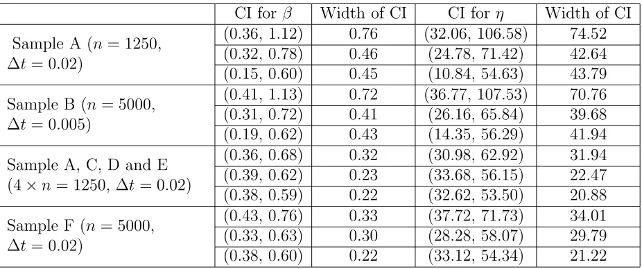
for this case. We use sample A as the benchmark. For Method 1, we obtain sample B by sampling every 5th data point in the first data set, so n = 5000 and ∆t = 0.005 for this case. We then use (2.18) and (2.19) to obtain the 95% CIs for β and η. For method 2, we sample every 20th data point in the 2nd to 4th data sets to get sample C, D, E and combine them with sample A to obtain 4 samples each of n = 1250 and ∆t = 0.02. For sample A, C, D and E combined together we have n = 5000 observations in total and ∆t = 0.02. We then use estimators from the regression model with more data sets using (2.30) and (2.31) to obtain the 95% CIs for β and η (with α = 0.05, zα/2 = 1.96). For method 3, we sample every 20th data point in the 5th data set to obtain sample F so n= 5000 and ∆t = 0.02 for this case. The results are displayed in Table 1.

We see from Table 1 that Method 1 (Sample B), using a sample from one location with denser observations, does not give smaller CIs for both β and η, while Method 2 (Samples A, C, D and E), using more samples at different locations, decreases the width of the CIs significantly and improves the efficiency of estimation. Method 3 (Sample F), using a sample with longer observations at one location, also gives narrower CIs. Therefore we conclude from this example that both Method 2 and 3 improve the efficiency of estimation. We have repeated our simulations with different model parameter values and the conclusions are the same.

Table 1: CIs for Example 2.6.1; results are repeated 3 times.

CI for β Width of CI CI forη Width of CI

Sample A (n = 1250, ∆t= 0.02)

(0.36, 1.12) 0.76 (32.06, 106.58) 74.52 (0.32, 0.78) 0.46 (24.78, 71.42) 42.64 (0.15, 0.60) 0.45 (10.84, 54.63) 43.79

Sample B (n= 5000, ∆t= 0.005)

(0.41, 1.13) 0.72 (36.77, 107.53) 70.76 (0.31, 0.72) 0.41 (26.16, 65.84) 39.68 (0.19, 0.62) 0.43 (14.35, 56.29) 41.94

Sample A, C, D and E (4_×n = 1250, ∆t= 0.02)

(0.36, 0.68) 0.32 (30.98, 62.92) 31.94 (0.39, 0.62) 0.23 (33.68, 56.15) 22.47 (0.38, 0.59) 0.22 (32.62, 53.50) 20.88

Sample F (n= 5000, ∆t= 0.02)

(0.43, 0.76) 0.33 (37.72, 71.73) 34.01 (0.33, 0.63) 0.30 (28.28, 58.07) 29.79 (0.38, 0.60) 0.22 (33.12, 54.34) 21.22

confi-dence region forβ and η for the regression model with m data sets of sizen as

mn∆t( ˆβ₋β)2+2√∆tX Xuij( ˆβ−β)(ˆη−η)+

X X

uij2(ˆη−η)2 ≤2ˆσ2Fα,2,mn−2, (2.32)

where ˆβ and ˆη are given in (2.27). We compute that

4∆tX Xuij

2

−4mn∆tX Xu2_ij = 4∆t X Xuij

2

−mnX Xu2_ij

!

. (2.33)

As for the regression model with one data set in section 2.5, we can prove that (2.33) is strictly negative. Therefore the boundary of the 100(1₋α)% joint confidence region for the regression model with m data sets is still an ellipsoid.

Example 2.6.2 Assume that the parameters are given by T = 1, I(0) = 10, β =

0.5, µ= 20, γ = 25, N = 100, m= 10 and σ2 _{= 0.03 for the model (1.2).}

We simulate I(t) using the above parameters by the EM method with a very small step size ∆t= 0.001, m= 10 times and save these I(t) as 10 sets of true data. Then we sample every 10th data in each data set to obtain 10 samples for our parameter estimation, so n = 100 and ∆t= 0.01 for each of our samples.

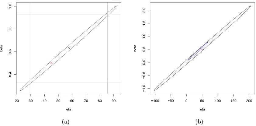
We find the boundary of the 95% joint confidence region for β and η using (2.33) and the univariate 95% CIs for each of them using (2.30) and (2.31), and also the point estimates using (2.27). These are shown in Figure 2(a).

We see that most of the ellipse lies in the square which represents the univariate CIs, but the area of the ellipse is much smaller than that of the square. This indicates the advantage of the joint confidence region, i.e. it does not include many of the extreme values in the univariate CIs and is more efficient. Also we see that the ellipse is centered at the point estimate of β and η. The red point which represents the true value of β= 0.5

and η= 45 lies in the ellipse.

Example 2.6.3 Assume that the model parameters are given by T = 1, I(0) = 10, β =

0.5, µ= 20, γ = 25, N = 100 and σ2 _{= 0.03 for the model (1.2).}

In order to examine the influence of different m on the 95% joint confidence region, we vary the value of m as m = 1, m = 2 and m = 5 and use the same method as in Example 2.6.2 to simulate data sets for each m and sample from each of them. We then obtain three 95% joint confidence regions for the different m, which are shown in Figure 2(b). We see that the area of the 95% joint confidence region becomes smaller as m becomes larger. Also the red point which represents the true value of β = 0.5 and η= 45 lies in all the ellipses.

3

Pseudo-Maximum Likelihood Estimation

In this context, the explicit expressions for MLEs for φ = (β, η, σ2_{) are not attainable,}

20 30 40 50 60 70 80 90

0.4

0.6

0.8

1.0

eta

beta

(a)

−100 −50 0 50 100 150 200

−1.0

−0.5

0.0

0.5

1.0

1.5

2.0

eta

beta

(b)

scheme, the Pseudo-likelihood method [3, 9], will be applied here to obtain estimators for β, η and σ2_{. We use the Euler method, which approximates the path of the process,}

so that the discretized form of the process has a likelihood that is usable and so can be maximised with respect to the parameter values.

3.1

Pseudo-MLE

The Euler scheme discretizes the process as (2.1). The incrementsIk+1−Ik are

condition-ally independent Gaussian random variables with meanIk(βN−η−βIk)∆t and variance

σ2_I

k2(N −Ik)2∆t. Therefore the transition density of the process can be written as

p(Ik+1,(k+ 1)∆t|Ik, k∆t)

= q 1

2πσ2_I

k2(N −Ik)2∆t

exp ₋ 1

2

[Ik+1−Ik−Ik(βN −η−βIk)∆t]2

σ2_I

k2(N −Ik)2∆t

!

, (3.1)

wherep(Ik+1,(k+ 1)∆t|Ik, k∆t) represents the conditional probability density thatI[(k+

1)∆t] =Ik+1 given thatI(k∆t) =Ik. Then a pseudo-likelihood is obtained as

Ln(φ) = n

Y

k=1





1

q

2πσ2_I

k2(N −Ik)2∆t

exp ₋ 1

2

[Ik+1−Ik−Ik(βN −η−βIk)∆t]2

σ2_I

k2(N −Ik)2∆t

!

.

(3.2) Taking the logarithm of (3.2) we have the log pseudo-likelihood

ln(φ) =−

1 2

X

[ln(2π∆t) +lnσ2+lnI_k2+ln(N ₋Ik)2]

− 1₂X[Ik+1−Ik−Ik(βN −η−βIk)∆t]

2

σ2_I

k2(N −Ik)2∆t

.

(3.3)

The corresponding partial derivatives with respect to β,η and σ2 _are

∂ln(φ)

∂β =−

XI_k+1−I_k−I_k(βN −η−βI_k)∆t

σ2_I

k2(N −Ik)2∆t

·(₋IkN∆t+Ik2∆t), (3.4)

∂ln(φ)

∂(η) =−

XI_k+1−I_k−I_k(βN −η−βI_k)∆t

σ2_I

k2(N −Ik)2∆t

·Ik∆t, (3.5)

∂ln(φ)

∂σ2 =− n

2σ2 +

1 (σ2₎2 ·

1 2∆t ·

X[I_k+1−I_k−I_k(βN −η−βI_k)∆t]2

Ik2(N −Ik)2

. (3.6)

By setting all the partial derivatives equal to zero and solving these simultaneously, we find ˆβ, ˆη and ˆσ2 where the pseudo-likelihood function changes direction. We find that

ˆ

β, ˆη have the same expressions as the least squares estimators in (2.7) and (2.8), while ˆ

σ2 _{is almost the same as the least squares estimator (2.14) except that it has n in the}

denominator instead of (n₋2). We notice that ˆβ, ˆη and ˆσ2 _{are a unique solution to the}

conclude that the turning point ( ˆβ, ˆη, ˆσ2_{) maximises the pseudo-likelihood function (3.2).}

Therefore ˆφ= ( ˆβ, ˆη, ˆσ2_{) are the pseudo-MLEs for (1.2).}

In the following sections we construct joint confidence regions for the pseudo-MLEs that we have obtained.

3.2

Exact Joint Confidence Region

We know that the pseudo-MLEs are exactly the same as the least squares estimators, except for a minor difference in the estimation ofσ2_{. If we want to find a joint 100(1−α)%}

confidence region forθ = (β,η) then we have already found this in the least squares case in (2.25) and (2.32) (for both m = 1 and m > 1) by obtaining an exact 95% confidence region for θ as

(θ₋θˆ)T var( ˆβ,ηˆ)−1σ2(θ₋θˆ)_≤σ2χ2_α,2, (3.7) where χ2

α,2 is the upperα point of the χ2 distribution on 2 degrees of freedom, and then

estimating σ2 _{by ˆσ}2_{. Note that we use ˆσ}2 _{in (2.14) instead of ˆσ}2 _{from the pseudo-MLE}

since the least squares estimator forσ2 _{is unbiased and is slightly better than the}

pseudo-MLE. Arnold (1998) [1] argues that if plug-in estimates are used for the variance, it is sensible to change the distribution from χ22 _{to 2F2}

,n−2 [4], to balance out the loss of

accuracy because of the substitution that increases the area of the region. We replace σ2

by ˆσ2 _{and therefore it is more sensible to use 2F}

2,n−2 here. Then it will lead to the same

analytic form of the 100(1₋α)% joint confidence region forβ and η as the least squares case in (2.24).

We already know the exact confidence region for β and η but we did not obtain the confidence region for all three pseudo-MLEs. In the following sections we construct large sample 100(1₋α)% joint confidence regions for all three pseudo-MLEs and for β and η

as well for purposes of comparison. There are two ways to construct the asymptotic joint confidence region. The first method is based on the assumption that the pseudo-MLEs are approximately multivariate normally distributed, while the second is based on the likelihood ratio test statistic.

3.3

Asymptotic joint confidence regions based on the

approxi-mate multivariate normality of pseudo-MLEs

We can regard one data point as X = (x0, x1, ..., xn), which is a complete run with the

initial data I0 and the transition probability as in (3.1). If we obtain m data points

X = (x0, x1, ..., xn) all with the same initial value and the same transition probability,

then our m observations are independently and identically distributed and all with the pseudo-likelihood function as given in (3.2). Within this framework, we can apply the asymptotic maximum likelihood theory.

If m = 1 (i.e. we have only one run) or m is very small this is not very helpful as the asymptotic theory requires the number of observations (m here) to be very large in order to be valid. In this case the estimators ˆβ and ˆη are exactly the same as in the least squares case. So ifσ2 _{is known their distribution is still exactly multivariate normal.}

the pseudo-MLE case. Ifm is large, we can then use the asymptotic pseudo-MLE theory and the likelihood ratio test which we will introduce in the next section.

First we find a joint confidence region for φ= (β,η,σ2_{). It is a standard result that}

the maximum likelihood estimators ( ˆβ, ˆη, ˆσ2_{) for (β,η,σ}2_{) are approximately}

multivari-ately normally distributed with mean φand variance 1

mΣ(φ)−

1_{, where Σ(φ) is the Fisher}

information matrix defined in (3.9) [1, 16, 20], i.e.

φ_{(m) ∼}N(3)

φ, 1 mΣ(φ)

approximately, (3.8)

where

Σ−1_{(φ) =σ}ij_{(φ) =}

−E

∂2

∂φ_i∂φ_jlnf(X;φ)

. (3.9)

Here

f(X;φ) =

n

Y

k=1





1

q

2πσ2_I

k2(N −Ik)2∆t

exp ₋ 1

2

[Ik+1−Ik−Ik(βN −η−βIk)∆t]2

σ2_I

k2(N −Ik)2∆t

!

,

so that

lnf(X;φ) =₋1 2

X

[ln(2π∆t) +lnσ2+lnI_k2+ln(N ₋Ik)2]

− 1₂X[Ik+1−Ik−Ik(βN −η−βIk)∆t]

2

σ2_I

k2(N −Ik)2∆t

.

The regularity conditions required are that

d dφ

Z

Ω

f(x;φ)dx=

Z

Ω ∂

∂φf(x;φ)dx (3.10)

where Ω denotes the sample space. This property follows from the conditional normal distribution of the increments Ik+1−Ik. For example

∂ ∂β

Z

Ω

f(x;φ)dx= 0

as the integral over the sample space is one. But

∂

∂βf(x;φ) =

n

X

k=1

θkf(x;φ), whereθk=

Ik+1−Ik−Ik(βN −η−βIk)∆t

σ2_I

k2(N −Ik)2∆t

·(IkN∆t−Ik2∆t),

for k = 1,2,3, . . . , n.

So

Z

Ω ∂

∂βf(x;φ)dx =

n

X

k=1

E(θk),

=

n

X

k=1 E

E(θk|I0, I1, . . . , Ik) ,

as the conditional distribution of Ik+1 − Ik given I0, I1, . . . , Ik is Gaussian with mean

Ik(βN −η−βIk)∆t and variance σ2Ik2(N −Ik)2∆t. The other two parts of (3.10)

corre-sponding to η and σ2 _{follow similarly.}

The quadratic form associated with (3.8),

U =

3

X

i=1 3

X

j=1

mσij(φ)( ˆφ_i−φ_i)( ˆφ_j−φ_j) (3.11)

has an approximate chi-square distribution with three degrees of freedom for large m. Because ˆφ is a strongly consistent estimate of φ, the statistics U will still have an asymptotic chi-square distribution with σij_{(φ) being substituted by σ}ij_{( ˆφ).}

This will give a three dimensional confidence region for φ = (β, η, σ2_{). To actually}

evaluate this asymptotic confidence region for our case is very complicated. The equation (3.9) is very difficult to calculate since it involves the approximation of E_(N 1

−Ik)2

, and also it will bring in extra error from the approximation, so we do not use this confidence region in our examples.

On the other hand we could assume thatσis known and that we are trying to estimate

θ = (β,η). This is parallel to the estimation procedure that we used in the least squares problem (estimating σ by ˆσ and getting a two dimensional confidence region for β and

η). Then

θ(m)∼N(2)

θ, 1 mΣ(θ)

approximately,

where

Σ−1_{(θ) = σ}ij_{(θ) =}

−E

∂2 ∂θi∂θj

lnf(X;θ)

. (3.12)

The associated quadratic form

U′ ₌

2

X

i=1 2

X

j=1

mσij(θ)(ˆθi−θi)(ˆθj−θj) (3.13)

has an approximate chi-square distribution with two degrees of freedom for large m. Note that ˆθ is the pseudo-MLE θˆ(σ) = ( ˆβ(σ),ηˆ(σ)) withσ known and solves

∂

∂βlnLn(θ) = 0 and ∂

∂ηlnLn(θ) = 0.

HereLn(θ) is given by (3.2) except that σ is regarded as known.

If σ is actually unknown, we can substitute σ by its least squares estimator ˆσ. Then the distribution for that statistic U′ _{is 2F2}

,mn−2 [4]. We should use mn−2 here rather

than m₋2 as the estimator ˆσ2 _{is the average of mn−2 sums of squares. Also we should}

use the least squares estimator, not the pseudo-MLE for ˆσ, for the same reason as in section 3.2, although the results using the pseudo-MLE will be very close. If m is large, 2F2,mn−2 will be approximately the same as a chi-square distribution with two degrees

of freedom and the asymptotic confidence region will then approach the exact confidence region.

3.4

Joint confidence regions based on the likelihood ratio

statis-tic

Another approximate confidence region is based on the likelihood ratio test statistic [1]. Suppose that we have m independent observations X1,X2, ...,Xm with common density

f(X_|φ). Then we can approximate the 100(1₋α)% confidence region forφ by

(φ:₋2logRn(φ)< χ23,1−α). (3.14)

Here

Rn(φ) =

Lm(φ)

Ln( ˆφ)

,

where the vector ˆφcontains the pseudo-MLEs for φ, the parameters,

Lm(φ) = m

Y

j=1

Ln,j(φ) (3.15)

and Ln,j(φ) = n

Y

k=1





1

q

2πσ2_I

k,j2(N −Ik,j)2∆t

exp ₋ 1

2

[Ik+1,j−Ik,j−Ik,j(βN −η−βIk,j)∆t]2

σ2_I

k,j2(N −Ik,j)2∆t

!

.

So a 100(1₋α)% confidence region forφ is

m

X

j=1

n

X

k=1

lnq 2

2πˆσ2_I

k,j2(N −Ik,j)2∆t

−lnq 2

2πσ2_I

k,j2(N −Ik,j)2∆t

+ [Ik+1,j−Ik,j−Ik,j(βN −η−βIk,j)∆t]

2

σ2_I

k,j2(N −Ik,j)2∆t

!

−mn < χ2α,3.

Again ifσ2_{is assumed known, a similar argument shows that a 100(1−α)% confidence}

region for θ is

m

X

j=1

n

X

k=1

[Ik+1,j−Ik,j−Ik,j(βN −η−βIk,j)∆t]2

σ2_I

k,j2(N−Ik,j)2∆t

− [Ik+1,j−Ik,j−Ik,j( ˆβN −ηˆ−βIˆ k,j)∆t]

2

σ2_I

k,j2(N −Ik,j)2∆t

!

< χ2_α,2.

(3.16)

Here again ˆθ is the pseudo-MLE ˆθ(σ) = ( ˆβ(σ),ηˆ(σ)) withσ known, and solves

∂

∂βlnLm(θ) = 0 and ∂

∂ηlnLm(θ) = 0.

In these equations Lm(θ) is given by (3.15) but regarded as a function of θ= (β, η) with

Again if we replace the unknown σ by ˆσ (the least squares estimator), then the distribution should be 2Fα,2,mn−2.

Then (3.16) can be written as

m X j=1 n X k=1

[Ik+1,j−Ik,j−Ik,j(βN −η−βIk,j)∆t]2

σ2_I

k,j2(N −Ik,j)2∆t

−(mn₋2)

!

<2Fα,2,mn−2,

which is equivalent to

1 ˆ σ2 m X j=1 n X k=1

(Ik+1,j−Ik,j)2

Ik,j(N −Ik,j)2∆t

+β2mn∆t+η2

m X j=1 n X k=1 ∆t

(N ₋Ik,j)2

+ηβ m X j=1 n X k=1

−2∆t N₋Ik,j

+β m X j=1 n X k=1

−2(Ik+1,j−Ik,j)

Ik,j(N −Ik,j)

+η m X j=1 n X k=1

2(Ik+1,j−Ik,j)

Ik,j(N−Ik,j)2

!

−(mn₋2)<2Fα,2,mn−2.

This can be simplified as

m X j=1 n X k=1

y2_k,j+β2nm∆t+η2

m X j=1 n X k=1

u2_k,j+ηβ2√∆t

m X j=1 n X k=1

uk,j+β(−2

√

∆t)

m X j=1 n X k=1 yk,j

+η(₋2)

m X j=1 n X k=1

uk,jyk,j−(mn−2)ˆσ2 <2ˆσ2Fα,2,mn−2,

with uk and yk defined in (2.2).

This can be written as

mn∆tβ₋βˆ2+

m X j=1 n X k=1

u2_j,k(η₋ηˆ)2+2√∆t

m X j=1 n X k=1

uk,j(β−βˆ)(η−ηˆ)<2ˆσ2Fα,2,mn−2−D,

(3.17) where

D=₋mn∆tβˆ2 ₋

m X j=1 n X k=1

u2_j,kηˆ2₋2√∆t

m X j=1 n X k=1

uk,jβˆηˆ+ m X j=1 n X k=1

y2_k,j−(mn₋2)ˆσ2.

The region (3.17) has the same form as the exact confidence region (2.32) apart from the substraction of a constantDon the right hand side. We have shown that (2.33) is strictly negative and therefore the 100(1₋α)% confidence region forθ (3.17) is an ellipse centered at the pseudo-MLE ˆβ and ˆη. We numerically compare the exact 95% confidence region forθ with the asymptotic confidence region obtained by using the likelihood ratio test in the following example, and establish the size of the difference D in this case.

Example 3.4.1 Assume that the parameters are given by T = 5, I(0) = 10, β =

0.5, µ= 20, γ = 25, N = 100, m= 100 and σ2 _{= 0.03for the model (1.2).}

42 44 46 48 50 52

0.48

0.50

0.52

0.54

0.56

0.58

eta

beta

(a)

42 44 46 48 50 52

0.48

0.50

0.52

0.54

0.56

0.58

eta

beta

(b)

Figure 3: (a) shows the exact 95% joint confidence region for β and η (2.32) using the parameter values in Example 3.4.1; (b) shows the approximate likelihood ratio based confidence region using (3.17).

4

Summary and Further Work

In this paper we have applied the pseudo-MLE and the least squares method to estimate the parameters in the stochastic SIS model. For the least squares method, we started with the case in which only one data set is available and then improved our method by considering the case where more than one data set is available. We have obtained the point estimators, 100(1₋α)% CIs and 100(1₋α)% joint confidence regions for β and η

for both cases. We also investigated which factors influence the width of the CIs and the areas of the confidence regions. Theorem 2.2 states that the asymptotic widths of the CIs for bothβ andη strictly decrease as the total time periodT increases and do not depend on the size of the time step ∆t. Example 2.6.1 shows that a sample from one location with denser observations does not give narrower CIs, while using more than one sample taken at different locations and getting a sample with a longer period of observation at one location decreases the width of CIs significantly and improves the efficiency of estimation. Examples 2.5.2 and 2.6.3 show that the area of the confidence region decreases with increasing total time period T and increasing number of samples m.

We have also obtained pseudo-MLEs which are almost the same as the point esti-mators from the least squares case, with a minor difference in the estiesti-mators of σ2_{. For}

calculated numerically the asymptotic confidence region based on the likelihood ratio test for β and η. Example 3.4.1 shows that the numerical asymptotic confidence region using the likelihood ratio test forβ and η is almost identical to the exact confidence region.

Comparing the least squares estimation method and the pseudo-MLE method, we find that although the pseudo-MLE is more popular for parameter estimation for SDEs, least squares estimation gave the same point estimators and joint confidence region as the pseudo-MLE and is easier to apply. In our case least squares estimation is advantageous. The Bayesian approach is another popular way to estimate the parameters for SDEs [9]. In practice, we often have some information about the value of parameters before data is collected. The Bayesian approach is advantageous in this circumstance since it includes the prior information about the model parameters in the form of one or more prior distributions [5]. We are applying the Bayesian approach to our stochastic SIS model and will report the results in a further paper.

References

[1] Arnold, B.C. and Shavelle, R.M., Joint confidence sets for the mean and variance of a Normal distribution, The American Statistician, 52(2)(1998), 133-140.

[2] Bishwal, J.P.N., Parameter Estimation in Stochastic Differential Equations, Berlin/Heidelberg: Springer-Verlag, 2008.

[3] Cao, J. and Hu, L., Asymptotic properties of a pseudo-MLE for CIR model, Pro-ceedings of the 2010 International Conference on IIGSS-CPS, Nanjing, China, Vol. 1: Advances on Probability and Statistics, 28-31 (2010), 206-209.

[4] Douglas, J.B., Confidence regions for parameter pairs, The American Statistican, 41(1) (1993), 43-45.

[5] Gelman, A., Carlin, J.B., Stern, H.S. and Rubin, D.B., Bayesian Data Analysis, London: Chapman and Hall, 1995.

[6] Gray, A., Greenhalgh, D., Hu, L., Mao, X. and Pan, J., A stochastic differential equation SIS epidemic model, SIAM Journal of Applied Mathematics, 71(3) (2011), 876-902.

[7] Gushchin, A.A. and K¨uchler, U., Asymptotic properties of maximum-likelihood-estimators for a class of linear stochastic differential equations with time delay,

Bernoulli, 5 (2000), 1059-1098.

[8] Hethcote, H.W. and Yorke, J.A.,Gonorrhea transmission dynamics and control, Lec-ture Notes in Biomathematics 56, Springer-Verlag, 1994.

[9] Iacus, S.M., Simulation and Inference for Stochastic Differential Equations with R Examples, New York: Springer, 2008.

[11] Kristensen, N.R., Madsen, H. and Young, P.C., Parameter estimation in stochastic grey-box model, Automatica, 40 (2004), 225-237.

[12] K¨uchler, U. and Kutoyants, Y., Delay estimation for some stationary diffusion-type processes, Scandinavian Journal of Statistics, 27 (2000), 405-414.

[13] K¨uchler, U. and Sorensen, M., A simple estimator for discrete-time samples from afine stochastic delay differential equations, Statistical Inference for Stochastic Processes, 13(2) (2010), 125-132.

[14] K¨uchler, U. and Vasil’jev, V.A., Sequential identification of linear dynamic systems with memory, Statistical Inference for Stochastic Processes, 8 (2005), 1-24.

[15] Lamb, K.E., Greenhalgh, D. and Robertson, C., A simple mathematical model for genetic effects in pneumococcal carriage and transmission,Journal of Computational and Applied Mathematics, 235(7) (2011), 1812-1818.

[16] Lindsey, J.K., Parametric Statistical Inference, Oxford: Clarendon Press, 1996.

[17] Lipsitch, M., Vaccination against colonizing bacteria with multiple serotypes, Pro-ceedings of the National Academy of Sciences, 94 (1997), 6571-6576.

[18] Mao, X., Stochastic Differential Equations and Applications, Chichester: Horwood Publishing, 2nd Edition, 2007.

[19] Mao, X. and Yuan, C., Stochastic Differential Equations with Markovian Switching, London: Imperial College Press, 2006.

[20] Mood, A.M.,Introduction to the Theory of Statistics, New York: McGraw-Hill, 1950.

[21] Nielsen, J.N., Madsen, H. and Young, P.C., Parameter estimation in stochastic dif-ferential equations: an overview, Annual Reviews in Control, 24 (2000), 83-94.

[22] Rawlings, J.O., Applied Regression Analysis: a Research Tool, Belmont, CA: Wadsworth, 1988.

[23] Reiß, M., Minimax rate for nonparametric drift estimation in affine stochastic delay differential equations,Statistical Inference for Stochastic Processes, 5 (2002), 131-152.

[24] Reiß, M., Nonparametric Estimation for Stochastic Delay Differential Equations, PhD thesis, Institut f¨ur Mathematik, Humboldt-Universit¨at zu Berlin, 2002.

[25] Reiß, M., Adaptive estimation for affine stochastic delay differential equations,

Bernoulli, 11 (2005), 67-102

[26] Timmer, J., Parameter estimation in nonlinear stochastic differential equations,

Chaos, Solitons and Fractals, 11, 2571-2578.