BLIND ADAPTIVE EQUALIZER FOR BROADBAND MIMO STBC
BASED ON PDF FITTING
Samir Bendoukha, Adel Daas, and Stephan Weiss
Centre for Excellence in Signal & Image Processing Department of Electronic & Electrical Engineering University of Strathclyde, Glasgow, G1 1WX, Scotland, UK
{samir,adel.daas,stephan}@eee.strath.ac.uk
ABSTRACT
In this paper, we propose a new blind adaptive technique used for the equalisation of space-time block coded (STBC) signals transmitted over a dispersive MIMO channel. The proposed approach is based on minimising the difference be-tween the probability density function (PDF) of the equalizer output — estimated via the Parzen window method — and a desired PDF based on the source symbols. The cost func-tion combines this PDF fitting with an orthogonality crite-rion derived from the STBC structure of the transmitted data in order to discourage the extraction of identical signals. This cost function motivates an effective and low-cost stochastic gradient descent algorithm for adapting the equaliser. The performance is demonstrated in a number of simulations and benchmarked against other blind schemes for the equalisa-tion of STBC over broadband MIMO channels.
1. INTRODUCTION
The use of multiple transmit and receive antennas, commonly known as MIMO, has been shown to increase the capacity of a transmission link, [1]. This extra capacity can be exploited to increase the diversity gain of the system. The work in [2] proposed the STBC transmit diversity scheme, which is ca-pable of maximising the diversity over frequency-flat MIMO channels, whose respsonses between pairs of transmit and re-ceive antennas can be characterised by a complex gain factor. For high data rate service, most channels cannot be con-sidered frequency-flat anymore but are dispesrive, causing inter-symbol interference. In order to exploit diversity in such an environment, a number of variations on the classical STBC encoding have been proposed. OFDM can decompose a frequency-selective channel by introducing subcarriers and a cyclic prefix into a number of individual narrowband trans-mission channels, which can each be STBC encoded [3, 4]. The drawback of OFDM systems is in general the sensitiv-ity to synchronisation errors and their large peak-to-average power ratio. Single-carrier time domain approaches were first proposed by [4], whereby the STBC structure was ap-plied to a window of symbols, which is, after a guard in-terval, repeated as a complex conjugate and time reversed version [5]. However, time-reversal (TR) STBC is sensitive if the channel is doubly-dispersive, e.g. frequency selective and time-varying [6].
A recently proposed blind equalisation scheme for STBC [6] overcomes this problem and shows a higher ro-bustness towards time-variations of the channel than TR-STBC. In order to increase the convergence speed of the STBC-CMA algorithm, various algorithmic variations have been evaluated recently, of which the most successful is the
recursive quasi-Newton (RQN) approach, [7]. Unfortunately, the RQN method requires a considerable computational ef-fort, which even a fast version of this algorithm cannot en-tirely aleviate.
In [8] a cost function that minimises the difference be-tween a measured PDF at the equalizer output and a target PDF has been proposed, assuming a simple Gaussian model for the desired pdf. The technique has been successfully applied for SISO equalisation [8, 9] and multiuser detec-tion [10]. In this paper we intend to apply PDF fitting to target the equalisation of an STBC MIMO system. Based on the STBC-CMA approach [6], the aim of this paper is to investigate a PDF fitting based cost function for the equalisa-tion of STBC over a broadband MIMO channel.
The paper is organised as follows. In Sec. 2 a brief de-scription of the channel and signal model is given. The pro-posed cost function for the equaliser is detailed in Sec. 3, which motivates the derivation of a stochastic gradient al-gorithm in Sec. 4 in order to update the equaliser coeffi-cients. Finally, Sec. 5 provides simulation results bench-marked against existing approaches to mitigate ISI in broad-band MIMO STBC systems. Finally, conclusions are drawn in Sec. 6.
The following notations are used in this paper: E{·}is
the expectation operator. Vectors and matrices are denoted by bold face lower- and uppercase variables, e.g.xandH,
respectively, and {·}∗,{·}T, and{·}H are the operators for complex conjugation, transposition and Hermitian transposi-tion.
2. CHANNEL AND SIGNAL MODEL
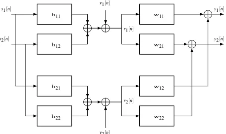
The general setup of channel and equaliser is outlined in Fig. 1, and the individual system blocks are described below.
2.1 Space-Time Block Coding
Assuming transmission from two transmit antennas, the transmit signal s[n]is STB encoded to provide two antenna signals si[n], i∈ {1,2}for the ith antenna, computed
accord-ing to [2],
s1[n] s1[n+1]
s2[n] s2[n+1]
=
s[n] −s∗[n+1]
s[n+1] s∗[n]
. (1)
This produces two orthogonal signals with a characteris-tic STBC structure, which will later be exploited in the equaliser.
w 22
g g
g
g g
-6
?
-? 6
-?
6
-6 6
-s1[n]
s2[n]
v1[n]
v2[n]
y2[n]
y1[n]
r1[n]
r2[n] h
22 h21 h
12
h11 w11
w 21
w12
g
Figure 1: Channel and signal model with transmit STBC sig-nals si[n], a 2×2 MIMO channel with CIRs hi j[n], received signals rj[n], equaliser components wj,i[n]and equaliser
out-puts yi[n]which should adhere to the STBC structure.
2.2 MIMO Channel Model
The receiver requires a minimum of two receive antennas in order to equalise the MIMO system characterised above. As-suming the availability of two sufficiently spaced receive an-tennas, the signals rj[n], j∈ {1,2}, received at the jth
re-ceive antenna over a dispersive and noise-corrupted channel are given by
r1[n]
r2[n]
=
N−1
∑
ν=0Hn
,ν
s1[n−ν]
s2[n−ν]
+vn
. (2)
The channel is characterised by the matrices
Hn
,ν=
h1,1[n,ν] h1,2[n,ν] h2,1[n,ν] h2,2[n,ν]
, (3)
whereby hj,i[n,ν]is the potentially time-varying channel
im-pulse response between the ith transmit and the jth receive antenna, responding to an inputδ[n−ν]. The vector
vn=
v1[n]
v2[n]
(4)
represents spatially and temporally uncorrelated Gaussian noise with zero mean and covarianceEv[n]vH[n] =σ2
vI. The parameter N in (2) is the length of the MIMO channel in (3) such thatHn
,ν=
0 ∀n≥N.
2.3 Equaliser
[image:2.595.52.280.72.208.2]For equalisation, we group the four subequalisers shown in Fig. 1 into two equaliserswi, i∈ {1
,2}, each responsible for
the ith output of the MIMO equaliser,
wi=
wi
,1
wi
,2
(5)
with
wH
i,j= [wi,j[0] ··· wi,j[L−1]], {i,j} ∈ {1,2}. (6)
Similarly, the received samples from the jth receive antenna sitting in the tap delay line of the subequaliser,
rT
j[n] = [r1[n]···r1[n−L+1]] , (7)
are concatenated into
r[n] =
r1[n] r2[n]
. (8)
With this notation, the outputs yi[n], i ∈ {1,2}, of the
equaliser in Fig. 1 over two successive symbol periods n and
n+1 can be written as
y1[n] y1[n+1]
y2[n] y2[n+1]
=
wH 1 wH 2
·[r[n] r[n+1]] . (9)
For successful equalisation, the equaliser output should match the channel input in an appropriate sense, and also re-flect the STBC structure in (1). We will use these properties to construct a suitable cost function next.
3. PDF-FITTING BASED COST FUNCTION
3.1 Cost Function Structure
The proposed cost function is based on the idea of blindly equalising several signals, leading to a cost term which is here related to fitting the PDFs of the equaliser outputs to a desired PDF according to [8, 11]. The danger of applying a blind criterion to every equaliser output yi[n] is that the strongest received signal will be extracted multiple times. In order to discourage multiple signal extraction, in [12] a cross-correlation criterion is added to the cost function. For STBC-CMA [6], this cross-correlation can be translated into an orthogonality conditionξ⊥of the two transmitted STBC signals. A similar approach is taken here, resulting in a com-bined cost function
ξ =α
NTx
∑
i=1
ξPDF,i+ (1−α)ξ⊥ (10)
whereξPDF,iis the criterion to force the ith output to attain a
specific desired PDF, with NTx=2 the number of transmitted symbols within the period of one STBC block. The param-eter 0≤α ≤1 controls the weighting between the two cost terms.
In the following, the PDF-fitting criterion for the extrac-tion of signals at the equaliser outputs yi[n] is outlined in Sec. 3.2, followed by comments on the orthogonality con-dition to discourage multiple signal extraction in Sec. 3.3.
3.2 PDF-Fitting Cost Function Component
The idea of this approach is to measure the difference be-tween two PDFs pA(z)and pB(z)[8],
ξPDF=
∞ Z
−∞
(pA(z)−pB(z))2dz . (11)
Here, the variable whose PDF is measured at the equaliser output is the squared magnitude value|yi[n]|2, in close rela-tion to the constant modulus algorithm. The estimarela-tion of this PDF is based on the Parzen window method, whereby a smooth PDF estimate is achieved by replacing a sample |yi[n]|2by a kernel function centred at its location. We here select a Gaussian kernel Kσ(z)with varianceσ,
Kσ(z) =√1 2πσe
−2z2σ2
such that the PDF estimate over a window of L output sam-ples is given by
ˆ
p|y
i[n]|2(z) =
1
L
L−1
∑
l=0
Kσ(z− |yi[n−l]|2) . (13)
The larger the window length L, the more confident the PDF estimate will be. However, a trade-off exists, as during adap-tation the output statistics are not sadap-tationary, therefore limit-ing L to an interval within which the statistics can be assumed quasi-stationary.
The PDF estimate ˆp|y
i[n]|2(z)will be compared to the PDF
of the squared moduli of the transmitted signals,|si[n]|2, sub-ject to the same Gaussian kernel Gσ(z)[9]. An advantage of convolving the discrete PDF of|si[n]|2defined by the constel-lation points of si[n]with the kernel is that the resulting PDF exhibits a spread around constellation points akin to the in-fluence of channel noise. Given the model of AWGN as out-lined in Sec. 2.2, the PDF of squared moduli would be a su-perposition of chi-square distributions, which subsequently might provide a more appropriate kernel. However, we here follow the suggestion of a Gaussian kernel in [9] as this will lead to simplifications that are required for a solution with low computational cost.
Therefore, the convolution with the Gaussian kernel yields the desired PDF
ˆ
p|s
i|2(z) =
1
M
M
∑
m=1
Kσ(z− |si,m|
2)
, (14)
where si,m, m∈ {1,2,···M}, are the M constellation points
of the ith transmitted signal.
By expoiting the fact that for Gaussian kernels [9]
∞ Z
−∞
Kσ(z−z1)Kσ(z−z2)dz=K√2σ(z1−z2) , (15)
the matched-PDF component of the cost function for the ith equaliser output simplifies for L=1 to, [8]
ξPDF,i[n] =−
1
M
M
∑
m=1
K√
2σ(|yi[n]| 2
− |si,m|
2)
. (16)
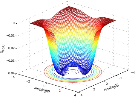
The cost function component in (16) is depicted in Figure 2 in dependency of a single complex valued coefficient. Simi-lar to the CMA, the cost function exhibits a manifold of op-timum solutions due to its phase ambiguity.
3.3 Orthogonality Condition
Applying the PDF matching criterion of Sec. 3.2 to both equaliser outputs could potentially lead to the multiple ex-traction of only the strongest signal. Therefore, an additional constraint such as the minimisation of the cross-correlation between the equaliser outputs needs to be included into the cost function [12]. The orthogonality of the STBC structure provides a good condition which does not require the approx-imation of the cross-correlation over a window of data, but can be directly applied to data collected over two consecu-tive time slots [6].
−4
−2
0
2
4 −4
−2 0
2 4 −0.04
−0.03 −0.02 −0.01 0
Real(wi [0]) Imag(w
i[0])
[image:3.595.309.535.84.246.2]ξPDF,i
Figure 2:The PDF-matching cost function for one output. Part of the surface has been removed to visualise the shape near the origine.
Based on (1), in the absence of noise and for perfect equalisation we have y1[n] =y∗2[n+1] =s[n] and y2[n] = −y∗1[n+1] =s[n+1]. Thus the vector
an=
y1[n] − y∗2[n+1]
y2[n] + y∗1[n+1]
, (17)
provides a suitable measure of orthogonality, such that
ξ⊥=aH
nan . (18)
If two orthogonal sequences are extracted, then the measure in (18) will be zero.
As the PDF-matching criterion is insensitive to the phase of the signals, the outputs yi[n] can be subject to an arbi-trary rotation commonly found with constant modulus-type algorithms. If we introduce a rotation angle ϕi for the ith equaliser output
an=
y1[n]ejϕ1 − y∗2[n+1]e−jϕ2
y2[n]ejϕ2 + y∗1[n+1]e−jϕ1
, (19)
and assume perfect equalisation yi[n] =si[n], then
aH
nan=0 ⇐⇒ ϕ1=−ϕ2+2πk (20) with k∈Z. Thus, if the total cost function is minimised, the phase ambiguity of the PDF fitting cost function compo-nent is complemented by (20), enforcing the orthogonality component such that the equaliser outputs can be expected to match the transmitted signals save of opposite phase shifts.
3.4 Overall Cost Function
With the PDF fitting and orthogonality condition defined, the complete cost function outlined in (10) can be approximated as
ˆ
ξn = −α
M
2
∑
i=1 1
∑
ν=0M
∑
m=1
K√2σ(|yi[n+ν]|2− |si,m|
2) +
+(1−α)aH
The PDF fitting component has an addition summation over two contributions, as the STBC code considered with (1) ex-tends over two symbol periods.
4. STOCHASTIC GRADIENT ALGORITHM
Based on the cost function in (21), this section addresses the problem of adjusting the equaliser. We choose a stochastic gradient approach whereby updating occurs for every STBC block spanning two symbol periods. The coefficients of the
ithequaliser are updated using the stochastic gradient descent method,
wi[n+2] =wi[n]−µPDF∇
w∗ i
ˆ
ξn, (22)
where∇w∗
i denotes the gradient with regard tow
∗
i, andµPDF is the step size.
The PDF and the orthogonality enforcing components of the gradient ˆξnare derived separately below.
4.1 PDF term
The derivative of the PDF term with respect to w∗
i can be given by
∂ ∂w∗
i
ξPDF|i[n]= 1
M
M
∑
m=1
K′√
2σ(|yi[n]| 2
−|si,m|
2)y∗
i[n]rn, (23)
where
K′√
2σ(z) =
∂
∂zK√2σ(z) =−
1
4σ2K√2σ(z) (24) is the derivative of the Gaussian kernel (12). In order to sim-plify the derivative, we assume all the points in the transmit constellation have the same modulus, i.e. |si,m|
2=γ2, for
m=1,···,M. Thus, the summation and division by M drops
form (23). Evaluating the derivative Kσ′ in (23) and rearrang-ing terms leads to
∂ ∂w∗
i
ξPDF|υ[n] =
K√
2σ(|yi[n]|
2−γ2)e∗[n]r
n υ=i
0 υ6=i,
(25) where,
e∗[n] = 1
4σ2(|yi[n]|
2−γ2)y∗
i[n], (26)
and K√2σ(z)is the Gaussial kernel used for the Parzen esti-mator as defined in (12) [9, 14]. It is the additional of this kernel term that distinguishes this part of the cost function gradient shown in (25) from a standard CM algorithm.
4.2 Orthogonality Condition
Note that the second part of the cost function (10), ξ⊥, is identical to the orthogonality-enforcing term of the STBC-CMA cost function. The gradient of the term with regard to the space-time equaliserswi, i∈ {1
,2}, is given by
∂ ∂w∗
1ξ⊥= (
y∗1[n]−y2[n+1])rn+(y2[n]+y∗1[n+1])rn+1
∂ ∂w∗
2ξ⊥= (y
∗
2[n]+y1[n+1])rn+(y2∗[n+1]−y1[n])rn+1.
(27) Inserting the combined terms (25) and (27) into (22) pro-vides the update equation of the proposed algorithm. The constants arising e.g. from the differentiation of the kernel can be absorbed into the step sizeµ.
[image:4.595.318.531.149.176.2]CMA RQN-CMA Matched-PDF 24Lw+4 36L2w+26Lw+59 24Lw+6
Table 1: Complexity of the different equalisers, in number of Multiply-Accumulate (MAC) operations.
[image:4.595.48.290.316.398.2]delay Ts 2Ts 3Ts 4Ts strength [dB] 0 −3 −5 −7 Table 2: Delay-power profile of the MIMO system’s channel impulse responses
5. ALGORITHM PERFORMANCE
This section provides details of the parameters of the algo-rithm and a comparison of its computational complexity, fol-lowed by simulations whose results are benchmarked against existing methods.
5.1 Computational Complexity
Tab. 1 lists the computational complexity of the proposed al-gorithm together with the STBC-CMA [6] and a fast con-verging, highly complex variant of the STBC-CMA based on a recursive Quasi-Newton update. The metric used here is to count complex multiply-accumulates (MAC). The differ-ence between the proposed algorithm and the STBC-CMA is the evaluation of the Gaussian kernel in the update equation. The Gaussian kernel can be approximated by a Maclaurin series with only relatively few MACs but poor behaviour for larger arguments to the kernel. The best results we obtained by implement the Gaussian function as a look-up table which requires memory and comparisons, but only one multiplica-tion.
5.2 Channel Simulation and System Parameters
A 2×2 MIMO model as indicated in Fig. 1 is used for sim-ulations. It comprises of four dispersive channel impulse responses of length Lh=4 obeying the delay-power pro-file characterised in Tab. 2. Simulations are performed over an ensemble of 100 MIMO channels whose coefficients are drawn from complex Gaussian distributions with variances defined by Tab. 2.
QPSK modulation is used at the transmitter with a mod-ulus equal to unity. At the receiver, signals are corrupted by AWGN at an SNR of 20dB.
The length of the subequaliserswi
,j, i,j∈ {1,2}is set to Lw=11, and they are initialised to zero with only the middle tap of each subequaliser set to unity. The trade-off between the two cost function terms was selected as α =0.4, and
the step sizes for the various algorithms were selected such that they provided the approximately fastest yet still stable convergence across all channel realisations.
5.3 Simulation Results
[image:4.595.50.290.475.542.2]0 500 1000 1500 2000 2500 3000 3500 4000 4500 5000 −45
−40 −35 −30 −25 −20 −15 −10
Iteration
MSE, [dB]
Matched−PDF CMA
[image:5.595.50.283.83.252.2]RQN−CMA
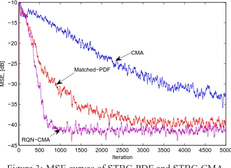
Figure 3: MSE curves of STBC-PDF and STBC-CMA.
5 10 15 20 25 30 101
102 103 104 105
Subequaliser Length, [L
w]
Complexity, [MACs] RQN−CMA
[image:5.595.50.287.271.376.2]CMA + PDF−Fitting
Figure 4: Complexity of the different equalisers, in number of Multiply-Accumulate (MAC) operations.
show that the MSE convergence of the PDF Matching Al-gorithm reaches the steady-state after fewer iterations com-pared to the STBC-CMA. The RQN equaliser shows the fastest convergence. However, as shown in Table 1, its com-plexity is of the order O(L2w) whereas the complexities of the STBC-CMA and the STBC-PDF schemes are of the or-derO(Lw). The complexity of the different equalisers is vi-sualised in Fig. 4 as a function of the subequaliser length
Lw. Both STBC-CMA and the proposed algorithm, have very similar computational cost.
6. CONCLUSIONS
A novel algorithm has been derived for the blind adaptive equalisation of STBC over frequency selective channels. The proposed cost function is based on minimizing the distance between the actual PDF of the equalizer output and a desired PDF, and is complemented by an additional term that ensures the STBC structure and hence orthogonality of the equaliser outputs. A low-cost stochastic gradient update was derived based on this cost function.
The complexity of the derived algorithm was found to be comparable to the STBC-CMA, but the proposed method exhibited a faster convergence close to the performance of the fast but very costly recursive quasi-Newton version of the STBC-CMA.
REFERENCES
[1] G. J. Foschini and M. J. Gans. “On limits of wire-less communication in a fading environment when
us-ing multiple antennas.,” in Wireless Personal
Commu-nications,, 6(3): 311335, March 1998.
[2] S.M Alamouti, “A simple transmit diversity technique for wireless communication,” in IEEE Selected Areas
in Communications., 16(8): 1451 1458, 1998.
[3] S. N. Diggavi, N. Al-Dhahir, A. Stamoulis, and A. R. Calderbank, “Differential space-time coding for frequency-selective channels,” IEEE Communications
Letters., 6(6): 253–255, June 2002.
[4] N. Al-Dhahir, “Overview and comparison of equaliza-tion schemes for space-time-coded signals with appli-cation to EDGE,” IEEE Trans. on Signal Processing., 50(10): 2477–2488, Oct. 2002.
[5] R. Schober, H. Z. B. Chen, and W. H. Gerstacker. “Decision-feedback sequence estimation for timerever-sal space-time block-coded transmission,” IEEE Trans.
on Vehicular Technology, 53(4): 127321278, July 2004.
[6] S. Bendoukha and S. Weiss “Blind CM equalisation for STBC over multipath fading,” IET ELECTRONICS
LETTERS, 44(15): 922923, July 2008.
[7] S. Bendoukha and S. Weiss “A Fast Converging Blind Receiver for Space-Time Block Codes over Frequency Selective Channels,” IEEE Int. Conf. on Signal
Pro-cessing and Comms, 169-172 , Nov. 2007.
[8] M. L´azaro, I. Santamar´ıa, D. Erdogmus, K. Hild, C. Puntale´on, and J. C. Principe “Stochastic blind equalization based on PDF fitting using Parzen estima-tor,” in IEEE Trans. on Signal Processing., 53: 696-704 , 2005.
[9] M. L´azaro, I. Santamar´ıa, C. Puntale´on, D. Erdog-mus, and J. C. Principe “Matched PDF-Based Blind Equalization,” in IEEE International Conference on
Acoustics, Speech, and Signal Processing ., 4: 297-300
, 2003.
[10] A. Daas, M. Hadef, and S. Weiss. “Adaptive blind mul-tiuser equalizer based on pdf matching,” In 16th Int.
Conference on Telecommunications., Marrakech,
Mo-rocco, May 2009.
[11] E. Gokcay and J. C. Principe. “Information theoretic clustering,” IEEE Trans. on Pattern Analysis and
Ma-chine Intelligence., 24(2):158–171, Feb. 2002.
[12] C. Papadias and A. Paulraj, “A Constant Modulus Al-gorithm for Multiuser Signal Separation in Presence of Delay Spread Using Antenna Arrays,” IEEE SP Let., 4(6):178–181, 1997.
[13] C. B. Papadias. “Unsupervised receiver processing techniques for linear space-time equalization of wide-band multiple input / multiple output channels,” in
IEEE Trans. on Signal Processing, 52(2): 472-482, ,
Feb 2004.
[14] S. Barbarossa and A. Scaglione, “Blind equalization using cost function matched to the signal constellation ,” in Asilomar Conference on Signals, Systems &
Com-puters., 1: 550-554, 1997.
[15] J. Sala-Alvarez and G. Vazquez-Grau, “Stastistical ref-erence criteria for adaptive signal processing in digital communications,” in IEEE Trans. on Signal