A practical engineering approach to the design and manufacturing of a mini kW blade wind turbine : definition, optimisation and CFD analysis

A Practical Engineering Approach to the Design and

Manufacturing of a mini kW Blade Wind Turbine: Definition,

optimization and CFD Analysis.

G.Frulla1, P.Gili1, M.Visone2, V. D'Oriano3 and M. Lappa4

Abstract A practical engineering approach to the design of a 60 kW wind generator with improved performances is presented. The proposed approach relies on the use of a specific, “ad hoc” developed software, OPTIWR (Optimization Software), expressly conceived to define an “optimum” rotor configuration in the framework of the blade-element-momentum theory. Starting from an initial input geometric configuration (corresponding to an already existing 50 kW turbine) and for given values of the wind velocity Vwind and of the advance ratio X = Vwind/ΩR (where Ω is the blade rotational

speed and R is the propeller radius), this software is used to determine iteratively the optimized distributions of chords and twists which can guarantee a constant value of the socalled axial induction factor a = 1/3 along the blade. The output configuration is then converted into a CAD model to be used, in turn, as input data for a CFD commercial software. With this tool the relative rotational motion between the fluid and the wind turbine are simulated resorting to a MRF (Moving Reference Frame) technique (for which continuity and momentum equations are solved in a rotating reference frame). The outcomes of the numerical simulations are then used to verify the improved performances of the optimized configuration and to which extent the CFD data agree with “expected” behaviours (i.e. performances predicted on the basis of the simplified model). Finally, some details about the construction technique used to turn the optimized configuration into an effective working prototype are provided, in conjunction with a critical discussion of suitable production methods for composite components.

Keywords: Wind turbine, optimum design; CFD simulation; manufacturing

1 _{Polytechnic University of Turin, Italy} 2,3 _{BLUE Engineering, Italy}

3 _{Corresponding Author}

1 Introduction

Wind turbines (WT) are generally categorized on the basis of the generated power (Burton et al.,2011). From a purely technical standpoint, this modus operandi leads to the following classification: a) “micro” ( power ≤ 20 kW), b) “mini” (≤ 200 kW ) c) “megawatt” (≤ 1.5 MW) and d) “Multimegawatt” (> 1.5 MW) turbines. From an engineering point of view, additional and more practical characterization of turbines can be obtained in terms of potential applications, relative importance of drawbacks and advantages, size/benefits ratio and so on.

As an example, it is well known that small and micro wind turbines represent a growing sector in the renewable energy field due to different “practical” applications involved. Indeed, these systems, are easily transportable, installable, maintainable, and can have an extremely wide geographical distribution (as they do not require special weather conditions to work effectively). Moreover, national incentive programs make these turbines easily accessible as well as an increasingly more affordable solution for consumers who want to reduce their environmental impact and their energy bills.

More specifically, micro turbines are characterized by small dimensions (of the order of 3-4.5 m) which make them particularly suitable for battery-charging (or similar) applications. Turbines of the Mini (or Small) kind are usually employed in small towns and/or in isolated areas where an electrical network is not available (most notably, they can be clustered in smart grid configurations).

Generally speaking, both Micro and small turbines can be regarded as simple systems which can be easily assembled and used for different technological prototype applications (Burton et al.,1011; IEC-2; Battisti, 2012).

Given such premises, the present paper is devoted to the definition, manufacturing and performance analysis of a typical wind turbine in the “mini” category.

some micro-turbines, such as those used on boats. Moreover, the small companies operating in the sector do not have the technical capacity or financial forces to sustain and implement research activities.

Until now, much has been done on the study and definition of the turbine airfoils in the context of aerodynamics research, at different Reynolds numbers (Somers, 1993;Ciguere and Selig, 1998; Miley,1982; Selig and McGranah, 2003). Moreover, some works have been appearing in the literature trying to address the problem related to the development of specific procedures to “control” (at a design level) the number of turbine revolutions as a function of the wind speed (Burton et al., 2011). Some exotic optimization strategies have been considered recently by Kriaa et al. (2011 and 2014).

An important aspect that has been overlooked until now, or at least not addressed in a systematic and generalized way, however, is the optimization of the blade geometry (in terms of chord and twist distribution along the radius).

Recently, Campobasso et al. (2014), presented a very interesting optimization strategy for the aerodynamic design of horizontal axis wind-turbine rotors including the variability of the annual energy production because of the uncertainty of the blade geometry caused by manufacturing and assembly errors. The used aerodynamic module was a blade-element momentum theory code.

Along these lines, the present work is devoted to the elaboration, application and “validation” of a practical strategy for blade wind turbine design and manufacturing based on a “predictor-corrector” philosophy (initial design theoretical optimization

CFD analysis corrections to be implemented in the initial design or at the optimization stage, if necessaryprototype manufacturing).

More specifically, the proposed approach relies on the use of a specific, “ad hoc” and “in-house” developed software, OPTIWR (In House Optimization Software), expressly conceived to define an “optimum” rotor configuration in the framework of a simplified model (i.e. under some simplifying assumptions which allow to define most of wind turbine properties on the basis of analytical relationships).

“input” data for a CFD commercial software. The outcomes of the numerical simulations are finally used to verify the improved performances of the optimized configuration and to which extent the CFD data agree with “expected” behaviours (i.e. performances predicted on the basis of the simplified model). Manufacturing by a composite construction technique (Frulla and Cestino, 2008) based on slender thin-walled structures is also discussed to a certain extent.

2 Preliminary design and optimization

One of the crucial phases in the classical design of new WT blades is the accurate prediction of the aerodynamic force coefficients of their aerofoils.These aerodynamic coefficients can then be used to calculate the force acting on the blades at each radius, and the radial integral of such forces determines both the overall torque (and thus the power).

We have selected the initial airfoil configuration on the basis of available data in the literature (Tangler and Somers, 1995; Somers, 2005). Following the literature, we have selected airfoils in the S series considering as well the possibility to combine different shapes: S819, S820, S821.

In particular, the three airfoils were combined in a specific configuration in which S821 was positioned in the first 40% of the radius, S819 up to about 75% of the radius and S821 in the remaining portion (Tangler and Somers, 1995). The corresponding airfoil aerodynamic data were collected and prepared for the OPTIWR. The available polars were analytically approximated in the range of useful angles of attack and in correspondence of at least four Reynolds numbers (the “system” or “global” Reynolds number is based here on the chord at 75% of the blade radius; hereafter, it is referred to as Re75% to avoid confusion with the local Reynolds number Re, based on the “local”

chord).

the "rough" ones in order to have a conservative calculation with respect to the "smooth" ones.

The OPTIWR program has been developed on the basis of well known Blade element momentum theory (BEMT). For the related details the reader is referred, e.g., to Hansen and Butterfield (1993), Walker and Jenkins (1997) and Hansen (2008). For the sake of completeness, here we will limit ourselves just to recalling that this theory is partially based on the “Actuator-Disk" model to account for the sudden rotation imparted by the flow by the actuator disk (Betz, 1922 and 1927).

The original theory relies on the assumption that a streamtube exists with fluid flowing through an actuator disk that represents the rotor (assumed to be infinitessimally thin). The gas interacts with the rotor, thus transferring energy from the fluid to the solid. The fluid then continues to flow downstream (accordingly, the system/streamtube can be ideally split into two portions: pre-acuator disk, and post-actuator disk). Before interaction with the rotor, the total energy in the fluid is constant. Furthermore, after interacting with the rotor, the total energy in the fluid is also constant. In the Blade Element Momentum theory, angular momentum is also included in the model.

According to this theory the system “efficiency” , defined as ratio of the power that can be effectively extracted from the fluid to the fluid overall power 1/2AV2 _{(where  is the}

fluid density, V is the fluid velocity, and A is the area of an imaginary surface through which the fluid is flowing) attains a maximum when the socalled axial induction factor a is 1/3 (this factor is related to the fluid velocity at the rotor via the expression Vrotor= Vwind

(1 - a) where Vwind is the asymptotic wind velocity).

Blade element theory also involves splitting the blade up into N elements. Each element will experience varying flow characteristics as they have differing rotational speeds (Ωr) and depending on the design, a differing chord (C) and twist distribution . The theory can be used to calculate the relative flow at each section and determine the overall performance characteristics by integrating along the span of the blade.

This theory, as reported in Hansen (2008) and Walker and Jenkins (1997) with all the necessary details, is at the basis of the OPTIWR software, which, starting from an initial input geometric configuration and for given values of Vwind and of the advance ratio X =

by a sort of “reverse engineering” (via subsequent iterations), the optimized distributions of chords and twists which can guarantee a constant value a = 1/3 along the blade.

A flow-chart showing the algorithm at the basis of the OPTIWR software is reported in figure 1 ( BET stands for Blade theory while MT stands for Momentum theory).

The initial requirements were defined in order to fulfill the following indications:

a) 60 kW of power produced at 8 m/s wind speed (which requires a rotor power of not less than 70 kW due to generator losses and other losses in the equipment).

b) A rotating speed of the rotor close to 50 rpm for 8 m/s wind speed and 70 kW power production.

c) Maximum efficiency attained for 5-5.5 m/s wind speed .

Accordingly, we have concentrated on X=8 with a design speed of 5 m/s. A three-blade rotor radius of 12.3 m has been identified as the best configuration for the production of 60 kW in nominal condition at 8 m/s wind speed.

a)

b)

Figure 3: Isometric view of the optimized 60 kW blade

a)

Table 1: Reference data

OPTIWR results Optimum Design point: X=8 Vwind=5 [m/s]

Power design point : X=8, Vwind=8 [m/s]

Efficiency  0.472 0.478

Power [W] 17188.5 71324.3

Torque [Nm] 5285.5 13707.6

Thrust [N] 5782.4 14810.5

Rotation speed [rpm] 31.05 49.69

The results are shown in Table 1 (hereafter, Vwind=5 m/s and Vwind=8 m/s are referred to

as the optimum design point and power design point, respectively).

Some small differences are evident mainly due to the variation of the Reynolds number for the two configurations. The design point (X=8, Vwind=5 m/s) was assumed as the

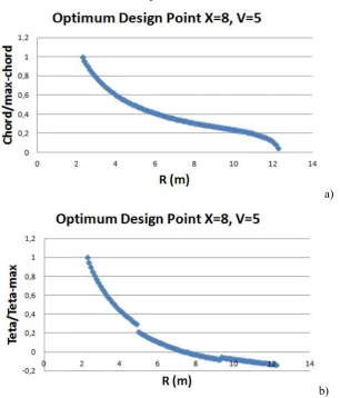
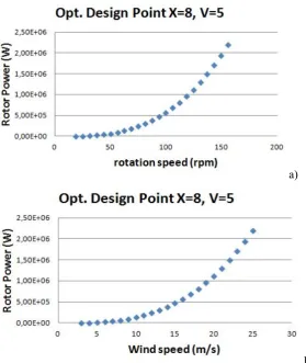
reference configuration in order to produce higher chord sizes. This secondary requirement was included for structural reasons, having in mind prototype manufacturing. The local non-dimensional chord behavior is reported in figure 2a while the twist is reported in figure 2b. The blade shape was derived by means of a CAD procedure on the basis of local airfoil chord and local twist. Figure 3 reports the blade external shape after regularization in the transition point. The CAD drawing data were prepared for the subsequent CFD analysis and for the last phase of manufacturing. The performance of the designed rotor is illustrated in figure 4a and 4b as a function of the rotation speed (4a) and versus wind speed (4b).

3 CFD Simulation and assessment of rotor performances

execution of the simulations using a CFD Commercial code (STAR-CCM+ 7.06.10), which solves a complete set of the Navier-Stokes equations.

3.1 Computational domain and grid

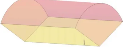
The computational domain is shown in Figure 5. It is assumed that the extension of the computational domain, is large enough compared to the length of the wing turbine, to prevent the flow field around the rotor blade from being affected by numerical external condition. The surface mesh has about 8x105 _{triangular elements, the volume is}

composed by 34.5x106 _{polyhedral cells. In order to model the boundary layer}

phenomena, about twenty prism layers have been extruded from rotor wall with a spacing near wall surface such as not to exceed 10 for the y+ value. Moreover several refinement blocks have been used (Figure 6).

Figure 5: Computational Domain

3.2 Physical and numerical model

Relative rotational motion between the flow field and the wind turbine was simulated using a MRF (Moving Reference Frame) technique, for which continuity and momentum equations are solved in a rotating reference frame, identified by setting a rotation axis and an angular velocity. Starting point for such a treatment is the realization that when the balance equations derived in in the ideal case of inertial system are transformed to a rotating frame of reference, the so-called Coriolis and centrifugal forces appear.

The mathematical expression of the Coriolis force per unit volume reads:

V

Fco 2



where, as usual,  and V are the density and velocity of the considered fluid particle, respectively, and  the constant angular velocity of the rotating frame of reference in which the fluid is considered.

The derivation of a mathematical expression for the other force, i.e. the centrifugal contribution, is less complex. It simply reads:

r Fce

2







where r=rir is the radial vector (r being the perpendicular distance from the axis of

rotation and ir the related unit vector).

The consideration of them in the Navier-Stokes equations in the framework of the incompressible-fluid approximation leads to the following expression in dimensional form (Lappa, 2012):

V r V p V V

V _{        }





_

_

_

_



t

2

2 ₍₄₎

Taking the curl of eq. (4) leads to the vorticity ( ) equation, which has proven to play a

very useful role in the analysis of rotating flows and is, therefore, reported here. Taking into account that the following vector identity holds

V V

V V

V    

  

 ( ) (5)

that V 0(incompressible fluid), that  is a constant vector (constant magnitude and

direction) and also considering the following vector identities:









  







2V V (6a)





  





 











 (6b)

the vorticity equation reduces to:



_



_

_











t (7)

Furthermore, the flow field was assumed steady and fully turbulent, (ρ=1.225 kg/m3 _and

T=const= 288 K, viscosity 1.78x10-5 _{Pa s).}

suggested by Rody (1991), allows the model to be applied in the viscous sublayer. In this approach the computation is divided into two layers. In the layer next to the wall, the dissipation rate  and the turbulent viscosity are specified as functions of wall distance. The values of  specified in the near-wall layer are blended smoothly with the values computed from solving the transport equation far from the wall. The equation for the turbulent kinetic energy k is solved for the entire flow.

3.3 CFD Tool Validation

A preliminary CFD analysis was carried out for an already existing 50 kW wind Turbine (figure 7) for the sake of numerical tool validation.

Simulations were carried for three different operating conditions to be compared with available experimental data.

Earlier experimental tests had provided the following operating data : the wind turbine rotational velocity Ω, the wind velocity measured by the Pitot probes VPitot and the disk

rotor electrical power. From the last quantity it was possible to deduce the aerodynamic power, and then the aerodynamic moment.

Numerical results have revealed that the wind velocity measured by the Pitot probes does not coincide with the real wind velocity Vwind, because the measure is affected by the fact

that the probes are positioned within the so-called central vortex (Figure 8 and figure 9).

For this reason CFD preliminary calculations were performed to find a correlation between the real wind velocity and the velocity measured by the Pitot.

In this calculations the numerical value of the latter quantity is intended to be the average value on the circumference passing through the probes and lying in the plane of normal X (figure 8 and figure 9), considering the axial symmetry of the model and the phenomenon cyclicality.

The study also included a sensitivity analysis, varying the wind velocity. Table 2 shows the correlation between Vwind and the VPitot for different operating conditions.

radius was 5 m, and the aerodynamic chord was 0.7952 m. CFD subsequent calculations were performed giving as input the Vwind coming out from the achieved correlation.

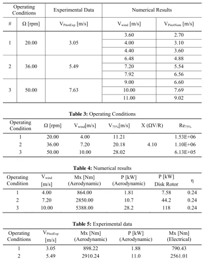
Tables 4 and 5 show the numerical and the experimental aerodynamic performances, respectively. The good agreement between the results, for all operating conditions, provides evidence for the reliability of the adopted fluid-dynamic model.

Figure 7: existing 50 kW wind Turbine

Table 2: Preliminary results

Table 3: Operating Conditions Operating

Condition Ω [rpm] Vwind[m/s] V75%[m/s] Χ (ΩV/R) Re75%

1 20.00 4.00 11.21

4.10

1.53E+06

2 36.00 7.20 20.18 1.10E+06

3 50.00 10.00 28.02 6.13E+05

Table 4: Numerical results Operating Condition Vwind [m/s] Mx [Nm] (Aerodynamic) P [kW] (Aerodynamic) P [kW]

Disk Rotor η

1 4.00 864.00 1.81 7.58 0.24

2 7.20 2850.00 10.7 44.2 0.24

3 10.00 5388.00 28.2 118 0.24

Table 5: Experimental data Operating Conditions VPitotExp [m/s] Mx [Nm] (Aerodynamic) P [kW] (Aerodynamic) Mx [Nm] (Electrical)

1 3.05 898.22 1.88 790.43

2 5.49 2910.24 11.0 2561.01

3 7.63 5613.89 29.4 4940.23

Operating

Conditions Experimental Data Numerical Results

# Ω [rpm] VPitotExp [m/s] Vwind [m/s] VPitotNum [m/s]

1 20.00 3.05

3.60 2.70 4.00 3.10 4.40 3.60

2 36.00 5.49

6.48 4.88 7.20 5.54 7.92 6.56

3 50.00 7.63

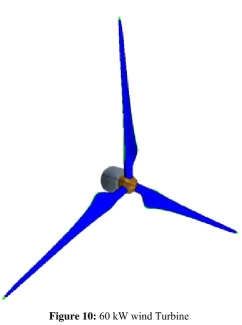
Figure 10: 60 kW wind Turbine

3.4 Results and Performances

Once validated the fluid-dynamic model, the CFD analysis on the 60 kW wind Turbine (Figure 10) was carried out for the two different operating conditions, in terms of wind velocity and wind turbine rotational velocity, already discussed in the foregoing sections (Table 6).

Velocity and Reynolds number have been evaluated at 75% of the blade radius, where the radius is 7.51 m, and the aerodynamic chord is 0.5604 m.

Tables 7 and 8 show the aerodynamic performances evaluated by means of CFD and OPTIWR, respectively. There is a good agreement between the results, for both the operating conditions.

turbine is characterized by better aerodynamic performances (Lindenburg, 2003; Hsiao et al.,2012) : its efficiency η is twice that of the existing 50 kW wind turbine.

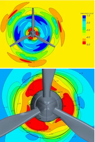
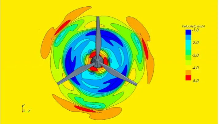
In particular Figure 11a and Figure 11b show the flow field on the probes plane for the different wind turbines providing clear evidence that the velocity field downstream of the 60 kW wind turbine is more uniform than that related to the 50 kW one.

Moreover Figure 12a and figure 12b reveal that the size of typical vortical structures downstream the 60 kW wind turbine tends to be smaller. Finally, a comparison of the pressure coefficient distributions on the upper and lower sides of the 60 kW turbine (Figure 13a, Figure 13b) and the existing 50 kW one (Figure 13c, Figure 13d) leads to the conclusion that on the former there are no cross-flow and re-circulation.

Table 6: 60 kW - Operating Conditions Operating

Condition Ω

[rpm] Vwind[m/s] V75%[m/s] _[ΩV/R]Χ Re75% VPitot[m/s] VPitot/Vwind

1 31.05 5.00 24.92 8.00 9.61E+05 4.50 0.90

2 49.68 8.00 39.88 8.00 1.54E+06 7.59 0.95

Table 7: 60 kW - Numerical results (CFD) Operating

Condition (Aerodynamic) Mx [Nm] (Aerodynamic) P [kW]

P [kW]

Disk Rotor η

1 5295 17219 36390 0.47

2 14100 73365 149051 0.49

Table 8 : 60 kW - Numerical results (OPTIWR code) Operating

Condition Mx [Nm] (Aerodynamic) P [kW] (Aerodynamic) η

1 5285 17189 0.47

Figure 11a: Flow Field on the Pitot plane: Existing 50 kW , Re=1.53x106

Figure 13a: Pressure coefficient on lower sides of the blade: 60 kW WT, Re=1.54x106

Figure 13c:Pressure coefficient on the upper side of the Existing 50kW blade, Re=1.53x106

Figure 14: 60 kW WT Prototype (Pictures)

3.5 Manufacturing

The configuration resulting from the above numerical study has been used as a relevant basis for manufacturing a working prototype (Figure 14).

A classical aerospace thin-walled solid/sandwich construction technique (traditionally employed for aerospace wing structures) has been used (Frulla and Cestino, 2008).

More specifically, the blade has been built by bonding two half-shells. Special care has been devoted not to alter the shape of the blade trailing edge (to avoid any possible reduction in aerodynamic efficiency due to geometrical departure from the optimal configuration).

It is also worth pointing out that, before shell bonding, internal structure reinforcements have been applied towards the end of reducing the maximum tip deflection under loads. Internal reinforcements have been introduced as well in correspondence of the airfoil external surface and in proximity to the root section (where changes in section shape are more significant).

Such additional structural elements have been built with the vacuum infusion method and the method of filament winding. For the convenience of the reader who is not an expert in typical production methods for composite components, let us recall that techniques to be used for such a purpose can be generally split into four main categories:

 Classic manual impregnation and lay-up

 The infusion method in closed mold (RTM - Resin Transfer Molding)

 Vacuum Infusion

 The prepreg molding with manual lay-up and vacuum bagged (PREG)

We have selected the resin infusion process (see, e.g., Potter, 1997) because it is with no doubt the best possible compromise between cost and final quality of the blade structure. Indeed, this technology is the most widespread one for the production of wind rotor blades and nacelle. It has been applied in combination with the vacuum infusion process (although this process requires relatively high investments, the final results are excellent both from the point of view of structural aspects and with respect to shape quality).

1. Preparation of the molds (treatment release);

2. Mold coating (gel-coat UV additive);

3. Application on the mold and the glass fiber core (tri-axial and expanded);

4. Application of drainage networks air;

5. Implementation of circuits for infusion and aspiration;

6. Mold closure with the infusion bag (polyethylene sheet);

7. Vacuum pump start;

8. Search and elimination of leaks;

9. Degree of vacuum and resin infusion (either epoxy polyester) tuning (in the case of epoxy resin the procedure follows the well known "cure phase");

10. Shells extraction from the molds (concave and convex shapes);

11. Shells bonding and reinforcement with structural bonders;

4 Conclusions

In this work, we considered the design of a typical 60 kW wind turbine pertaining to the “medium size” category. This class of turbines can be regarded as an interesting opportunity in the recent field of green energy generation for the possibility to take advantage of modern smart-grid and design concepts. Starting from already existing theories, the design activity consisted of the identification of the best chord and pitch distributions for the blade in defined operating conditions.

Acknowledgements : The research described in this paper was financially supported in the framework of a contract between the Department of Mechanical and Aerospace Engineering at the Polytechnic University of Turin (Italy) and Sorel S.r.l. (“Progetto Aerodinamico di Rotore per Aerogeneratore da 60 Kw”, 2013 research contract). The authors would like to thank Prof. Salvatore D'Angelo for some helpful discussions and the theoretical support provided during the numerical-algorithm definition stage.

References:

Battisti L., (2012), “Scelta e istallazione delle mini turbine eoliche”, Speciale Tecnico di www.qualeenergia.it, Feb. 2012.

Benjanirat S. and Sankar L., (2003), “Evaluation of turbulence models for the prediction of wind turbine aerodynamics” AIAA paper 0517, 2003.

Betz A., (1922), "The Theory of the Screw Propeller", NACA TN 83 Betz A., (1927), "Propeller Problems", NACA TM 491

Burton T., Sharpe D., Jenkins N., Bossanyi E, (2011), “Wind Energy Handbook”, Second Edition, John Wiley&Sons, LTD, New York, USA.

Campobasso M.S., Zanon A., Minisci, E. and Bonfiglioli A. (2009), “Wake-tracking and turbulence modelling in computational aerodynamics of wind turbine aerofoils”, Proceedings of the Institution of Mechanical Engineering, Part A: Journal of Power and Energy, Vol. 223 (8). pp. 939-951 - ISSN 0957-6509.

Campobasso M. S., Minisci E., Caboni M, (2014), “Aerodynamic design optimization of wind turbine rotors under geometric uncertainty”, Wind Energy 11/2014, http://dx.doi.org/10.1002/we.1820

Ciguere P. and Selig M. S., (1998), “New airfoils for small horizontal axis wind turbines”, Transactions of the ASME, Vol. 120, pp. 108-114.

Frulla G. and Cestino E., (2008), “Design, manufacturing and testing of a HALE-UAV structural demonstrator”, Composite Structures, Vol. 83, pp. 143-153.

Hansen M., (2008), “Aerodynamics of Wind Turbines”, Earthscan, London, Sterling, VA.

Hansen A. and Butterfield C., (1993), “Aerodynamics of horizontal-axis wind turbines”, Annual Review of Fluid Mechanics, Vol. 25, pp. 115-149

IEC 61400-2 – “Wind Turbines, Part 2: Design Requirements For Small Wind Turbines”.

Kaminsky C., Filush A., Kasprzak P., Mokhtar W., (2012), “CFD Study of Wind Turbine Aerodynamics”, Proceedings of the 2012 ASEE North Central Section Conference.

Kriaa M., El Alami M., Najam M. and Semma E., (2011), “Improving the Efficiency of Wind Power System by Using Natural Convection Flows”, Fluid Dyn. Mater. Process. (FDMP), Vol. 7, No. 2, pp. 125-140.

Kriaa M., El Alami M., and Abouricha M., (2014), “Contribution to Improving the Performance of a Wind Turbine Using Natural Convection Flows”, Fluid Dyn. Mater. Process. (FDMP), Vol. 10, No. 4, pp. 443-464.

Lee H. M. and Chua L.P., (2012), “Investigation of the stall delay of a 5kW horizontal axis wind turbine using numerical method” International Conference on Renewable Energies and Power, Santiago de Compostela (Spain), 28th to 30th March, 2012.

Lindenburg, C., (2003), “Investigation into rotor blade aerodynamics”, 2003, ECN-C-03-025, Netherlands.

Mayer R. M., (1993), Design with reinforced plastics, Springer, ISBN 978-0-85072-294-9, 228 pp.

Miley S. J.,(1982), “A catalog of low Reynolds number airfoil data for wind turbine applications”, Department of Aerospace Engineering Texas A&M University, RFP-3387, UC-60.

Potter K., (1997), Resin Transfer Moulding, Springer Netherlands, 264 pp.

Rodi W., (1991), “Experience with Two-Layer Models Combining the k- Model with a One-Equation Model Near the Wall”, 29th Aerospace Sciences Meeting, January 7-10, Reno, NV, AIAA 91-0216.

Selig M.S., McGranah B.D.,(2003), “Wind tunnel aerodynamic tests of six airfoils for use on small wind turbines” National Renewable Energy Laboratory, Jan. 2003. NREL/SR-500-34515.

Somers D.M., (2005), “The S819, S820, and S821 Airfoils”. NREL/SR-500-36334. Somers D.M.,(1993), “The S819, S820, and S821Airfoils”, National Renewable Energy Laboratory, State College, Pennsylvania, December 1993.

Tangler J.L., Somers M.D., (1995), “NREL Airfoil families for HAWTs”, NREl/I'P-442-7109 - UC Category: 1211 - DE95000267.

USER GUIDE STAR-CCM+, (2012) Version 7.06 - CD-ADAPCO