False Discoveries: Winners and Losers in Mutual Fund Performance

      

City, University of London Institutional Repository

Citation

:

Cuthbertson, K., Nitzsche, D. and O'Sullivan, N. (2008). False Discoveries: Winners and Losers in Mutual Fund Performance. London: SSRN.

This is the published version of the paper.

This version of the publication may differ from the final published

version.

Permanent repository link:

http://openaccess.city.ac.uk/16849/

Link to published version

:

Copyright and reuse:

City Research Online aims to make research

outputs of City, University of London available to a wider audience.

Copyright and Moral Rights remain with the author(s) and/or copyright

holders. URLs from City Research Online may be freely distributed and

linked to.

FALSE DISCOVERIES: WINNERS AND LOSERS IN

MUTUAL FUND PERFORMANCE

Keith Cuthbertson*, Dirk Nitzsche* and Niall O’Sullivan**

This version : 5th January 2008

Abstract:

We use a multiple hypothesis testing framework to estimate the false discovery rate (FDR) amongst UK equity mutual funds. For all funds, we find a relatively high FDR for the best funds of 67% (at a 10% significance level), which indicates that only around 2% of all funds truly outperform their benchmarks. For the worst funds the FDR (at a 10% significance level), is relatively small at 15.9% which results in 20% of funds which truly underperform their benchmarks. For different investment styles, this pattern of very few genuine winner funds is repeated for all companies, small companies and equity income funds. However, forming portfolios of funds based on a set of funds for which the FDR is relatively low, produces positive alphas.

Keyword : Mutual fund performance, false discovery rate. JEL Classification : C15, G11, C14

* Cass Business School, City University, London, UK

** Department of Economics, University College Cork, Ireland

Corresponding Author:

Professor Keith Cuthbertson, Cass Business School, 106 Bunhill Row, London, EC1Y 8TZ. Tel. : +44-(0)-20-7040-5070,

FALSE DISCOVERIES: WINNERS AND LOSERS IN

MUTUAL FUND PERFORMANCE

1. Introduction

In the US and UK about 70% of institutional funds are actively managed and this rises to

over 90% for retail funds. Tests of the performance of active mutual funds are important for

investors choosing between active and index funds and for the broader question of the validity of

the EMH, given that the mutual fund industry appears to be highly competitive with low barriers to

entry and plentiful information available at relatively low cost. It is well documented that the

average US or UK equity mutual fund underperforms its benchmarks (Elton, Gruber, Das and

Hlavka 1993, Wermers 2000, Quigley and Sinquefield 2000, Fletcher 1997). However, the

cross-section standard deviation of the alphas for individual funds in both the UK and US is high,

indicating the possibility that some funds are performing very well and others very badly (Malkiel

1995, Kosowski et al 2006, Cuthbertson, Nitzsche and O’Sullivan 2008). In the US and UK the

latter results are not overturned by the addition of market timing variables or the use of

conditional alpha-beta models, as these “additional variables” when added to unconditional factor

models appear to be statistically insignificant (Treynor and Mazuy 1966, Henriksson and Merton

1981, Ferson and Schadt 1996, Fletcher 1995, Leger 1997).

In this paper we examine the performance of individual funds and address the question of

how many actively managed UK funds we truly expect to have an (ex-post) abnormal net return

performance (after adjustments for risk) which is positive, negative or zero.

The standard approach to determining whether the performance of a single fund (or a

single portfolio such as the average fund) demonstrates skill or luck is to choose a rejection

region and associated significance level

γ

and to reject the null of “no outperformance” if the test

statistic lies in the rejection region - ‘luck’ is interpreted as the significance level chosen.

However, using

γ

= 5% when testing the alphas for each of m-funds, the probability of finding at least one lucky fund from a sample of m-funds is much higher than 5% (even if all funds have true

alphas of zero)1. Put another way, if we find 20 out of 200 funds (i.e. 10% of funds) with

significant positive estimated alphas when using a 5% significance level then some of these will

merely be lucky – indeed 5% of all true null-funds found to be significant, will be false positives.

(The false positive rate is the probability that the fund’s performance is found to be significant,

given that it is truly null). One method of dealing with the possibility of false discoveries is to test

each of the m-funds independently but use a very conservative estimate for the significance level

of each test - for example the Bonferroni test would use

γ

/

m

= 0.000125. This would ensure that the overall error rate in testing m-funds (known as the Family Wise Error Rate) is controlled

at

γ

- but the danger here is in excluding funds that may truly outperform2.

In testing the performance of many funds a balanced approach is needed - one which is

not too conservative but allows a reasonable chance of identifying those funds with truly

differential performance. An approach known as the false discovery rate (FDR) attempts to strike

this balance by classifying funds as “significant” (at a chosen significance level

γ

) and then asks the question, “What proportion of these significant funds are false discoveries?” – that is, are

truly null (Benjamini and Hochberg 1995, Storey 2002 and Storey, Taylor and Siegmund 2004).

The FDR measures the proportion of lucky funds among a group of funds which have been found

to have significant (individual) alphas and hence ‘measures’ luck among the pool of ‘significant

funds’. For example, suppose the FDR amongst 20 significant best/winner funds (e.g. those with

positive alphas) is 80% then this implies that only 4 funds (out of the 20) have truly significant

1

This probability is the compound type-I error. For example, if the m tests are independent then Pr(at least 1

false discovery) = 1 – (1- γ )m = zm , which for a relatively small number of m=50 funds and conventional γ=0.05 gives

zm = 0.92 – a high probability of observing at least one false discovery.

2

Holm (1979) uses a step down method which uses significance level γ/m for the lowest p-value fund and

alphas3 - this is clearly useful information for investors. So, truly informed investors when forming

portfolios need to know both the size of the significant alphas of individual funds and also the

FDR amongst these alphas.

The competitive model of Berk and Green (2004) suggests that entry and exit of funds

should ensure that in equilibrium there are neither funds with long-run positive nor negative

abnormal performance. The US mutual fund industry has been extensively analyzed and

although the UK fund market is smaller, our sample of around 650 UK equity funds provides a

large comprehensive independent data set, thus mitigating possible claims of data snooping bias

if results are only based on repeated analysis of US data4.

In this paper we estimate the FDR for all UK mutual funds, for different style categories

and we also estimate the FDR separately for funds with positive and negative alphas. The

change in the FDR as the level of significance changes also allows us to determine whether the

truly best and worse performing funds are concentrated or dispersed in the tails of the

distribution.

The FDR has been used to analyze US equity mutual funds (Barras, Scaillet and

Wermers 2005) while here we use UK data and extend the analysis to consider the performance

of portfolios of mutual funds formed on the basis of the FDR statistic. For example, as the

significance level is increased, we will obtain more “significant funds” but if this is accompanied by

an increase in the FDR, many of these significant funds may be merely lucky – in forming

3

We use the usual language and terminology found in the statistical literature on false discoveries and error rates. The use of the word “truly” (sometimes “genuine” is used) should not be taken to mean that we are 100% certain that a proportion of funds among a particular group of significant funds have non-zero alphas – the FDR even if it is found to be zero, is still subject to estimation error. Also note that the FDR says nothing about the statistical significance of the alpha of any particular individual fund - conceptually, the FDR only applies to a group of significant funds. The FDR approach seems to have been first used in testing the difference between genes in particular cancer cells Storey (2002) and has recently been used in the economics literature to test alternative exchange rate models McCracken and Sapp (2005) and to test the performance of US equity mutual funds (Barras, Scaillet and Wermers 2005).

4

In other developed countries the mutual fund sector is generally less mature and smaller than in the US and UK

portfolios of funds it may therefore be prudent to include a small number of significant funds

which have a low FDR rather than form a larger portfolio of significant funds but having a higher

FDR. We therefore estimate the number of best and worst performing funds while controlling the

overall FDR. This allows us to identify a subset of funds for which the FDR is less than some

chosen value, say 10% and provides the investor with a subset of significant funds to include in a

fund-of-funds portfolio, for which she has set the FDR at an acceptable level. We then estimate

the expected alpha for this portfolio.

In summary, this paper adds to the UK mutual fund literature by analyzing the robustness

of the FDR approach and how it may give different inferences from the standard approach of

“counting” the number of significant funds. We also apply the FDR approach to portfolio

formation and determine the expected alpha from a set of funds which have a maximum FDR set

at a predetermined level. Our key results are that there is a much higher proportion of false

discoveries among the best funds than among the worst funds – so the standard method of

simply counting the number of funds with “significant” test statistics can be far more misleading

for “winners” than for “losers”. We find few funds which truly outperform their benchmarks and

these are concentrated in the extreme right tail of the performance distribution, whereas there are

a far greater number of genuinely poor performing funds, which are spread throughout the left tail.

This result holds for different investment styles, so there are few winners in any of our style

categories but there are far fewer equity income funds that are truly poor performers, relative to

the number of poor performers in either the All Companies or Small Company sectors. If we

control the overall FDR at say 10% then from our set of significant funds, there are a maximum of

20 truly winner funds (3% of all funds) and about 4 times more loser funds (13% of all funds) - but

the majority of funds neither statistically beat nor are inferior to their benchmarks and therefore

appear to do no better on a risk adjusted performance then merely tracking their style indexes5.

5

Using US data Kosowski et al (2006) measure the role of luck in mutual fund performance using p-values of the

The rest of this article is organized as follows. In section 2 we discuss the methodology

behind the FDR and other methods of controlling for false positives in a multiple testing

framework. In section 3 we outline our data set and in section 4 we evaluate the evidence on UK

equity mutual fund ex-post performance and section 5 concludes.

2. Methodology : The False Discovery Rate

Most previous work either tests the performance of the average fund or uses the

standard procedure of independently testing each fund’s performance and stating the number of

funds with significant alphas (hence assuming the FDR is zero). The null hypothesis is that fund-i

has no abnormal performance with the alternative that the fund delivers either positive or negative

performance:

0

:

i

H

α

=

0

H

_A

:

α

_i

>

0

or

α

_i

<

0

[Table 1 here]

The issues that arise in multiple testing of m-funds of which are truly null and are

truly alternative can be demonstrated using table 1 (Storey 2002). We call a fund’s performance

significant whose p-value for the test statistic (e.g. t-statistic on alpha) is less than or equal to

some threshold

0

m

m

₁

γ

(

0

< ≤

γ

1

). The number of false positives (sometimes referred to as lucky

funds) and the number of significant funds

F

R

are:

[1a]

F

( )

γ

=

#{

p

i

≤

γ

|

H true

₀

}

i

=

1,.... ...,

m

[1b]

R

( )

γ

=

#{

p

i

≤

γ

}

We wish to estimate the false discovery rate FDR, which for large m is given by:

[2]

FDR

( )

γ

=

E F

[ ( ) / ( )]

γ

R

γ

≈

E F

[ ( )] / [( ( )]

γ

E R

γ

An estimate of

E R

[ ( )]

γ

is the observed number of significant funds

R

( )

γ

, but

E F

[ ( )]

γ

is unobservable. However,

E F

[ ( )]

γ

=

m

₀

γ

=

π

₀

m

.

γ

where

π

₀= is the proportion of truly null funds. The proportion of true null funds is also unobservable but to provide an estimate

of

0

/

m

m

0

π

we can use the result that truly alternative features are clustered around zero, whereas

truly null p-values are uniformly distributed. The simplest method to estimate

π λ

ˆ ( )

₀ is to choose

a value

λ

for which the histogram of p-values becomes flat and to calculate

π

₀ using:

[3]

π λ

ˆ ( )

₀ =

#{

}

(1

)

i

p

m

λ

λ

>

−

If the histogram of p-values is perfectly flat to the right of our choice of

λ

then the

estimate of

π

₀ is independent of

λ

. So, if we were able to count only truly null p-values then [3]

would give an unbiased estimate of

π

₀ - but if we erroneously include a few alternative p-values

then [3] provides a conservative estimate of

π

₀ and hence of the FDR. Of course if we set

1

λ

=

then

π λ

ˆ ( )

₀ = 1 which is far too conservative.

For finite m, it can be shown that the bias in the estimate of

π λ

ˆ ( )

₀ is decreasing in

λ

but its variance increases with

λ

. An alternative method of estimating

π

₀ is to plot

π λ

ˆ ( )

₀

the smoothing method. A third method of estimating

π

₀ is to exploit the bias-variance trade-off

and choose

λ

to minimize the mean-square error

E

{

π λ π

₀

( )

−

₀

}

2 - this we refer to as the bootstrap method (which is outlined in the appendix). Having estimated

π

₀ the estimate of the

FDR is6 :

[4]

( )

ˆ

0

( ) .

ˆ

0

( ) .

( )

#{

_i

}

m

m

FDR

R

p

π λ

γ π λ

γ

γ

γ

γ

=

=

≤

The FDR can be applied to a two-sided test with equal-tailed critical values. However, we

can also partition the

R

significant funds into

R

+ with significant positive alphas (i.e. best or

winner funds) and

R

− with significant negative alphas (i.e. worst or loser funds). By definition

false positives (lucky funds)

F

( )

γ

are drawn from the null distribution so we expect half of them to have positive and half of them negative alphas, hence we can estimate the FDR for the best

and worst funds (Barras, Scaillet and Wermers 2005) :

[5a]

( )

[0.5 ( )]

( )

E

F

FDR

R

γ

γ

γ

+ +

=

=

0.5 .

ˆ

0

( ).

#{

_i

}

m

p

π λ γ

γ

+

=

≤

[5b]

( )

[0.5 ( )]

( )

E

F

FDR

R

γ

γ

γ

− +

=

0.5 .

ˆ

0

( ).

#{

i

}

m

p

π λ γ

γ

−

=

≤

where

p

_i+ and

p

_i−are the p-values of the best (

α

_i>0) and worst (

α

_i< 0) funds. Barras et al

(2005) use a Monte Carlo study on the CAPM model to show that the estimators outlined above

are accurate, are not sensitive either to the method used to estimate

λ

or to the chosen

significance level - while Storey, Taylor and Siegmund (2004) show that estimators of the FDR

6

This requires R( )γ >0, hence the term “positive FDR” is also used. We do not make this distinction since

( ) 0

are robust to many forms of dependence in the estimated p-values (e.g. dependence in finite

blocks).

Controlling the FDR

Low p-values indicate stronger evidence against the null and the p-value is the minimum

possible false positive rate for which we reject H0 – but adopting a very low significance level can

be too conservative. To avoid a too conservative approach to inference, we may wish to isolate a

set of funds such that among these funds the overall FDR is less than or equal to some desired

threshold value. Intuitively this process can be described as follows. We wish to choose the

minimum FDR amongst a group of funds for which we will reject H0 – this is known as the q-value.

If we order the p-values in a ‘list’ from lowest to highest

p

₍₁₎

≤

p

₍₂₎

≤ ≤

...

p

_{( )}m then we can

associate with each ordered p-value, a statistic which gives the overall FDR for the set of

funds with p-values less than . Note that the have the same ordering as the . For

example, if we choose a desired FDR of 10%, then we find that position in our list corresponding

to = 0.10 - for which there will also be an associated p-value, say 0.02. We know that if

we take all funds with 0.10 (all of which will have p-values less than or equal to 0.02)

then the overall FDR among those funds will be no more than 10%. Put another way,

thresholding at 10% may give 150 funds that are significant but we can now infer that a

maximum of only 15 are expected to be false positives

( )

(

_i

q p

)

)

)

i

q p

)

( )i

p

q p

(

_{( )i}

p

_{( )i}

( )

(

_i

q p

( )

(

)

≤

( )

(

i

q p

7

. The algorithm used to calculate the

q-values is described in an appendix.

Calculation of the FDR depends on correct estimation of individual p-values. Because of

non-normality in regression residuals we use a bootstrap approach to calculate p-values of

estimated t-statistics (Politis and Romano 1994). Consider an estimated model of equilibrium

7

Note that = 0.10 does not imply that fund-i has a probability of 10% of being a false positive. Because

the threshold q-value includes funds which are more significant than fund-i, the probability that fund-i is a false positive

( )

( _i)

returns of the form: for i = 1,2,…,m funds, where = number of

observations on fund-i, = excess return on fund-i, = vector of risk factors, are the

residuals and is the (Newey-West) t-statistic for alpha. For our ‘basic bootstrap’ we use

residual-only resampling, under the null of no outperformance (Efron and Tibshirani 1993). First,

estimate the chosen factor model for each fund and save the vectors

,

ˆ

ˆ

'

ˆ

i t i i t i t

r

=

α β

+

X

+

e

,

T

i

t i

r

,

X

t

e

ˆ

i t,

ˆ

_i

t

{

β

ˆ ˆ

i

,

e

i t,

}

. Next, draw a

random sample (with replacement) of length from the residuals and use these re-sampled

bootstrap residuals to generate a simulated excess return series under the null

hypothesis (

i

T

e

ˆ

_{i t,}

t i

e

,

~

t i

r

,

~

i

α

= 0). Then, using the performance model is estimated and the resulting

t-statistic for alpha, is obtained. This is repeated B =1,000 times and for a two-sided,

equal-tailed test the bootstrap p-value for fund-i is:

t i

r

,

~

b i

t

[6] 1 1

1 1

ˆ

ˆ

2.min[

(

),

(

)]

B B

b b

i i i

b b

p

B

−

I t

t

B

−

I t

t

= =

=

∑

>

∑

i

<

i

where I(.)is a (1,0) indicator variable.

3. Performance Models and Data

Our alternative performance models are well known ‘factor models’ and therefore we only

describe these briefly. Each model can be represented in its unconditional, conditional-beta and

conditional alpha-beta form. Unconditional models have factor loadings that are time invariant.

Carhart’s (1997) four-factor (4F) model is:

[7]

r

_{i t,}

=

α β

_i

+

_{1i m t}

r

_,

+

β

_2i

SMB

_t

+

β

_3i

HML

_t

+

β

_4i

MOM

_t

+

ε

_{i t},

where is the excess return on fund-i (over the risk-free rate), is the excess return on the

market portfolio while , and

,

i t

r

r

m t,

t

SMB

HML

_t

MOM

_t are factor mimicking portfolios for size,

book-to-market value and momentum effects, respectively. The Fama and French (1993) 3F model

includes only { , , } and has mainly been applied to UK funds (e.g. Blake and

Timmermann 1998, Quigley and Sinquefield 2000, Tonks 2005) but for US funds Carhart (1997)

finds that momentum is also statistically significant.

t m

r

,

SMB

t

HML

t

In conditional alpha-beta models it is assumed that alpha and the factor betas may

depend linearly on lagged public information variables

Z

_t and for the CAPM this gives:

[8]

r

_{i t,+1}

=

α

_0i

+

A z

_i'

( )

_t

+

b r

_0i

(

_{b t,+1}

)

+

B z

_i'

( *

_t

r

_{b t, 1+}

)

+

ε

_{i t,+1}

where is the excess return on a benchmark portfolio (i.e. market portfolio in this case) and

is the vector of deviations of

, 1

b t

r

₊

t

z

Z

t from its unconditional mean. Conditional-beta models

(Ferson and Schadt 1996) set

A

_i'

=

0

. Following earlier studies (Ferson and Schadt 1996, Christopherson, Ferson and Glassman 1998) our Zt variables include permutations of: the

one-month T-Bill yield, the dividend yield of the market factor and the term spread.

Our mutual fund data set comprises UK equity Unit Trusts and Open Ended Investment

Companies (OEICs) and represent almost the entire set of UK equity funds which have existed at

any point during the sample period under consideration, April 1975 – December 20028. By

8

Mutual fund monthly returns data have been obtained from Fenchurch Corporate Services using Standard &

restricting funds to those investing in UK equity, more accurate benchmark factor portfolios may

be used in estimating risk adjusted abnormal performance. We have removed ‘second units’ and

index/tracker funds leaving only actively managed funds. The equity funds are categorized by the

investment objectives of the funds which include: equity income (162 funds), ‘all companies’ (i.e.

formerly general equity and equity growth, 553 funds) and smaller companies (127 funds). The

data set includes both surviving funds and non surviving funds.

All fund returns are measured gross of taxes on dividends and capital gains and net of

management fees. Hence, we follow the usual convention in using net returns (price to

bid-price, with gross income reinvested). The market factor used is the FT All Share Index of total

returns (i.e. including reinvested dividends). Excess returns are calculated using the one-month

UK T-bill rate. The factor mimicking portfolio for the size effect, SMB, is the difference between

the monthly returns on the Hoare Govett Small Companies (HGSC) Index and the returns on the

FT 100 index9. The value premium, HML, is the difference between the monthly returns of the

Morgan Stanley Capital International (MSCI) UK value index and the returns on the MSCI UK

growth index10. The factor mimicking portfolio’s momentum behavior, MOM, has been

constructed using the constituents of the London Share Price Database, (total return) index11.

Other variables used in conditional and market timing models include the one-month UK T-bill

rate, the dividend yield on the FT-All Share index and the slope of the term structure (i.e. the yield

on the UK 20 year gilt minus the yield on the UK three-month T-bill).

9

The HGSC index measures the performance of the lowest 10% of stocks by market capitalization, of the main

UK equity market. Both indices are total return measures.

10 _{These indices are constructed by Morgan Stanley who rank all the stocks in their UK national index by their}

book-to-market ratio. Starting with the highest book-to-market ratio stocks, these are attributed to the value index until 50% of the market capitalization of the national index is reached. The remaining stocks are attributed to the growth index. The MSCI national indices have a market coverage of at least 60% (more recently this has been increased to 85%). Total return indices are used for the construction of the HML variable.

11

For each month, the equally weighted average returns of stocks with the highest and lowest 30% returns, over

4. Empirical Results

We begin with a discussion of our preferred factor models. Next we discuss alternative

estimation methods for the proportion of truly null funds among our m-funds

π

₀, then we analyze

the FDR for all our funds as well as the winner and loser funds taken separately – this allows us

to ascertain whether such funds are concentrated in the tails of the performance distribution.

Next we discuss the FDR for our three investment styles. Finally, we examine the number of

winner and loser funds in a set of funds for which we control the overall FDR to a chosen

“acceptable” level and we examine the sensitivity of the number of truly winner and loser funds

across the four different factor models used in our analysis.

Preferred Models

In this section, alternative performance models are examined. All tests are conducted at

a 5% significance level unless stated otherwise and results presented relate to all UK equity

mutual funds over the period April 1975 – December 2002 and are based on 675 funds with a

minimum of = 36 observations. For each model, cross-sectional (across funds) average

statistics are calculated. A single ‘best model’ is chosen from each of the 3 model classes; (i)

unconditional, (ii) conditional-beta and (iii) conditional alpha-beta, using the Schwartz Information

Criterion (SIC) and these results are reported in table 2.

min ,

i

T

[Table 2 here]

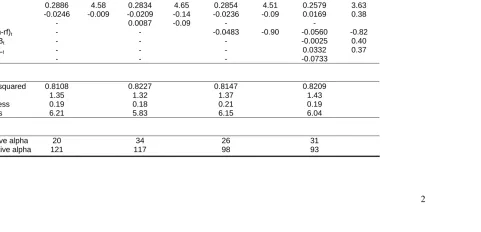
In the best three models (bottom half of table 2), the cross-sectional average alpha takes

on a small and statistically insignificant negative value (consistent with Blake and Timmermann

1998). However, of key importance for this study (and for investors) is the relatively large

cross-sectional standard deviations of the alpha estimates which is around 0.26% p.m. (3.1% p.a.), for

the unconditional and conditional-beta models and somewhat larger at 0.75% p.m. for the

conditional alpha-beta model. This implies that the extreme tails of the distribution of abnormal

performance may contain a substantial number of funds. This is important since investors are

more interested in holding funds in the right tail of the performance distribution and avoiding those

in the extreme left tail, than they are in the average fund’s performance.

The excess market return, , and the factor betas are consistently found to be

statistically significant across all three classes of model, whereas the

t m

r

_,

SMB

HML

factor beta is often

not statistically significant, even at a 10% significance level (as discussed further at the end of the

next section). We find that the momentum factor (

MOM

) is generally not statistically significant

at the individual UK fund level (e.g. Blake and Timmermann 1998, Tonks 2005), in contrast to US

studies (Carhart 1997). For the conditional-beta model (2nd column, table II) only the dividend

yield variable produces near statistically significant results. In the conditional alpha-beta model

we find that none of the conditional alphas has a t-statistic greater than 1.1 but some of the

conditional betas are bordering on statistical significance and our best model is shown in column

3.

The above results suggest that the unconditional Fama-French 3 factor model explains

UK equity mutual fund returns data reasonably well. These findings are consistent with existing

UK studies (Quigley and Sinqefield 2000, Fletcher 1995). Turning now to diagnostics (bottom

half of table II), the adjusted R2 across all three models is around 0.8, while the average

skewness and kurtosis of the residuals is around 0.2 and 6 respectively and more than 60% of

funds have non-normal errors (Bera-Jarque statistic – not reported here). The Schwartz

Information Criterion (SIC) is lowest for the unconditional 3F model. The Fama-French 3 factor

model was selected as the ‘best model’ for all three categories: unconditional, conditional beta

and conditional alpha-beta model but because the 4F model is widely used for US equity mutual

funds, we also report some variants using this model12.

12

The market timing models of Treynor-Mazuy (1966) and Henriksson–Merton (1981) are not as good as the 3F

Estimating

π

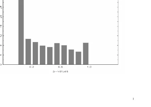
₀ and the FDR

The histogram of p-values is given in figure 1 for the unconditional 3F-model. Exploiting

the fact that truly null p-values are uniformly distributed [0,1] the height of the flat portion of the

histogram gives a conservative estimate of

π

₀. We cannot know that all p-values to the right of

any chosen

λ

(the x-axis of figure 1) are truly null but inclusion of a few alternative p-values

makes our estimate conservative. For finite m, the bias in our estimate

π λ

ˆ ( )

₀ is decreasing in

λ

but its variance increases with

λ

and hence from figure 1 a reasonable estimate would be

λ

= 0.5 giving

π λ

ˆ ( )

₀ = 0.72. Alternative estimates given by the smoothing and the bootstrap

techniques for the four different factor models are given in table 3.

[Figure 1 here]

[Table 3 here]

Looking down the four columns in table 3 we see that for any given factor model the

estimate

π λ

ˆ ( )

₀ is reasonably constant across the three different estimation methods. For three

of the four factor models, the 3 alternative estimation methods give reasonably similar estimates

of

π λ

ˆ ( )

₀ of around 75-85% but for the Carhart 4F model

π λ

ˆ ( )

₀ is somewhat lower and in the

range of 62-64%. However, the FDR also depends on the number of significant funds which will

vary across each factor model, so the different estimates of

π λ

ˆ ( )

₀ need not translate into

different estimates of the FDR – as we see below. The results indicate a large proportion of true

null funds in our sample (that is funds with

α

_i = 0) - overall, around 75% of active funds yield truly

zero alphas13.

But what proportion of “significant funds” (for any chosen significance level) have truly

differential performance? For reasons of brevity and clarity we first report detailed results for the

unconditional 3F model (which is the best ‘in sample’ model) using the bootstrap estimate

π λ

ˆ ( )

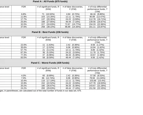
₀

= 0.72 and report results for other models in an appendix. Table 4 gives estimates of the FDR,

the number of significant funds R, the number of funds from among the R-funds that are false

discoveries, F and the number that are estimated to be truly significant T, at each significance

level

γ

(ranging from 0.01 to 0.20). Panel A gives result for all funds while Panels B and C report results for the best and worst funds, respectively.

[Table 4 here]

The standard approach indicates a relatively large number of significant funds for

example, for

γ

= 0.10 this amounts to 188 funds (27.8% of all funds). However, the FDR is quite high at 25.8% so 48 of these significant funds (7.18% of all funds) are false discoveries leaving

140 funds (20.67% of all funds) as having truly differential performance. There is a clear

difference of interpretation between the standard approach and one that takes account of false

discoveries. Indeed as the significance level is increased above 10% there is a danger in picking

up a substantial number of additional significant funds, most of which are false discoveries. For

example, as we move from

γ

= 0.10 to

γ

= 0.15 then the increase in significant funds is 39 but only about one-third of these (14), have truly differential performance.

With

γ

= 0.01 the FDR is 6.8% and there are R = 71 (out of 675 funds) that are significant (panel A) with only F = 5 being false discoveries and T = 66 having truly differential

performance. As

γ

increases the FDR increases. However, a significance level of

γ

= 0.025 gives an estimated FDR = 11.8% while

γ

= 0.05 gives a “reasonably acceptable” FDR = 17.7%

0

ˆ ( )

π

13

Barras et al (2005) using data on US funds (and the unconditional 4F model) estimate

λ

to be around

corresponding to a number of funds with differential performance of 91 and 113 respectively.

Above this significance level the number of funds that are false discoveries rises at a faster rate

than the number of significant funds so the FDR rises to quiet high (and probably unacceptable)

levels.

Best and Worst Funds

The most striking feature about the performance of the best and worst funds revealed by

our analysis of the unconditional 3F model is the relatively high

FDR

+ for the best funds and low

for the worst funds – this is true for any significance level chosen (Table 4, Panels B and

C). For example for

FDR

−

γ

= 0.05, of the

R

=137 significant funds only

R

+ = 21 have significant

positive alphas while

R

− = 116 have significant negative alphas. But given that = 58% is

much higher than = 10%, only 9 (1.3% of all 675 funds) have truly positive alphas (Panel

B). So, the standard approach indicates

FDR

+

FDR

−

R

+= 21 funds have significant positive alphas but this

“simple count” does not incorporate false discoveries, which implies only 9 funds truly outperform.

Although very few best funds truly outperform their 3F benchmarks this number does not rise with

γ

indicating that around T+ = 10 best funds (about 1.5% of all funds) are concentrated in the

extreme right tail of the performance distribution. The increase in the number of significant best

funds

R

+ as

γ

increases, is therefore due to the large number of false discoveries - as indicated

by the rapid increase in

FDR

+ (Table 4, Panel B).

The standard approach gives a relatively more accurate picture of the performance of the

worst funds. For example, for

γ

=0.05, the

FDR

− is relatively small at 10.4% so of the

R

− = 116 significant worst funds, about 104 (15.4% of all funds) have truly negative alphas (Panel C).

/

)

T

−

m

increases with

γ

, indicating that the poorly performing funds are fairly evenly spread

throughout the left tail of the performance distribution in the interval

γ

=

[0, 0.15]

(Panel C)14.

Style Categories

It is useful for investors to know if different style categories give different results for the

performance of the best and worst funds after taking account of the FDR15. It turns out that

although there are some minor differences, the broad qualitative results found when analyzing all

mutual funds apply to the separate style categories. For each of the three styles we find a high

for the best funds, a low

FDR

+

FDR

− for the worse funds and a relatively high overall FDR (for

all significance levels). Therefore we only report results for the three style categories using

γ

= 0.05 (full results are available on request).

[Table 5 here]

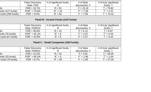
For the “all companies” sector with 423 funds in total16, the overall FDR (for

γ

= 0.05) is relatively low at 16.7% which with R = 91 funds found to be significant, gives 75 funds which truly

have differential performance. However, for the positive-alpha funds

FDR

+= 76% so only 2-3 of

the best all companies funds are truly significant but with

FDR

−= 9.4% most (i.e. 73) of the worst

“all companies” funds truly underperform their benchmarks. This pattern is broadly repeated for

the 109 smaller company funds with

FDR

+= 65% and

FDR

− = 7% which implies that out of R =

32 significant funds (for

γ

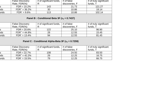
= 0.05) only one fund has a truly positive alpha while 27 have truly

14 _{These results for the unconditional 3F model are robust across our 4 different factor models and these results}

are reported in the appendix. We also estimate FDR, FDR+ and FDR- recursively from 1990 and found no discernable trends in our estimates, indicating that the FDR has been reasonably constant. Also our results for UK funds are broadly similar to those for ‘all’ US equity funds (1975-2002). Barras et al (2005) find a FDR of 55% among the 52 ‘top’ funds (at a 5% significance level), so only 23 of these (which constitutes 2% of all funds) have genuine skill and they all lie in the extreme right tail of the alpha-distribution. They find around 20% of all funds have genuinely ‘bad skill’ and these funds are spread throughout much of the left tail (and across all investment styles).

15

In order to calculate the FDR we used π0 estimate based on all funds as m needs to be ‘large’. The results

negative alphas. For equity income funds the situation is a little different because = 32%

is not too dissimilar to =42%, so the number of truly positive and negative funds which

outperform are approximately equal. Unfortunately there are few significant equity income funds

so the number of genuine outperformers (and underperformers) is around 4

FDR

+

FDR

−

17

.

Overall, the results show that only a handful of best funds from any of the different styles

have truly positive alphas, while there are a relatively large number of the worst funds in the all

companies (73) and smaller company (27) sectors with truly negative alphas. But the

performance of the worst equity income funds is mainly due to bad luck as only 3 funds have truly

poor performance. For investors, use of the FDR demonstrates that it is much more difficult to

find winners than would be indicated by the standard approach.

Controlling the Overall FDR

Instead of simply estimating the false discovery rate among our funds, we can instead

choose a “threshold” FDR and find a sub-set of funds which have an overall FDR which is less

than this chosen threshold “q-value”. The q-value threshold sets an upper bound on the

proportion of funds with “significant” alphas, that turn out to be false leads. We test the

robustness of this approach across our 4 factor models.

[Table 6 here]

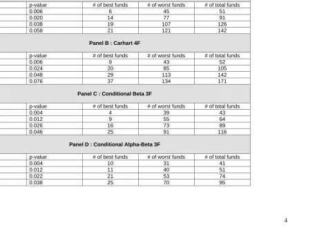
Panels A-D of table 6 show the number of best and worse funds which lie below a

chosen threshold q-value (together with the associated maximum p-value), for each of our four

factor models. For example, for the unconditional 3F-model and a threshold q-value of 0.10, we

find 91 funds that are significant with 14 having positive alphas and 77 negative alphas – all of the

aforementioned funds have a p-values of 0.02 or smaller. Therefore to control the overall FDR to

16

To obtain a p-value for each fund, we only included funds with a minimum number of observations of 36. That

a maximum of 10% we would choose a cut-off p-value for funds which we call “significant”, of

0.02 - much lower than the conventional p-value cut-offs of 0.05 or 0.10 used to test each fund

taken in isolation. This is because when testing many funds for differential performance we

require a lower p-value cut-off value in order to control the overall FDR at our chosen level.

As might be expected, for the different factor models there is some statistical variability in

the number of (best and worst) funds that are “significant” after controlling for the overall FDR, but

this variability is not particularly large. For example, for all 675 funds, when controlling the FDR

at 5% (10%) the number of best funds which can be taken to be significant across the four

models lie between 4 and 9 ( 9 and 20) and the number of worst funds range between 31 and 43

(40 and 85). Thus if you are willing to accept a maximum FDR of 10% among funds you call

significant, then there are a maximum of 20 truly winner funds (3% of all funds) and about 4 times

more loser funds (13% of all funds) and this result is fairly robust across our 4 different factor

models.

Portfolios of Best and Worst Performers

It is natural for an investor to be interested in the expected value of the alpha of a

portfolio of funds among which the maximum FDR is chosen at some desirable pre-set level, say

q = 10%. There is no guarantee that such a portfolio will have a high (absolute) alpha since a

fund could have a low q-value because the standard error of alpha is small relative to alpha itself.

For a conservative estimate of this portfolio alpha we form equally weighted portfolios of either

the best or worst funds, from the set of funds for which the q-value is less than 10%. We report

the expected value of alpha

E

α

_q

=

0.9

α

ˆ

q, where

α

ˆ

q is the estimated value of the best or worst

portfolio alpha for each of our 4 models18. (This portfolio contains a changing number of funds

over time for each of the different models).

17 _{The results for small companies and income funds must be interpreted with caution and can be no more than}

indicative, since we need m large to ensure that the distribution of null p-values approaches a uniform distribution.

18

The expected value is Eαq= −(1 FDR q( ))αA+FDR q( )α0 where αAand α0are the values under the null

[Table 7 here]

Table 7 shows that across the 4 models, the expected alpha for the best funds varies

between 4.57% p.a. (bootstrap t = 5.4) for the Carhart 4F model to 10.1% p.a. (bootstrap t = 4.12)

for the 3F-conditional beta model. For the worst funds the expected alphas are much less

variable across the 4 models with all alphas being close to -3.6% p.a. (with t-stats greater than

7)19. Part of the reason for the greater variability in alpha (and lower t-statistics) for the “best

portfolio” is that the latter contains an average of only about 5-10 funds (across different models),

whereas the “worst portfolio” has an average of around 35-50. However, overall it appears that

choosing a best or worse portfolio with a maximum FDR of 10% gives expected alphas which are

economically significant.

It is not possible to unambiguously compare the above method with the “standard

method” since both require an arbitrary chosen “cut-off” point for fund selection. Nevertheless as

a reasonable point of comparison consider the standard method of including (best or worst) funds

in your portfolio if they have p-values less than the “conventional”

γ

= 5%. The expected alpha

is

E

α γ

( )

=

{[1

−

FDR

( )]

γ α

_A20

where

α

_A is the population alpha under the alternative

hypothesis and

FDR

( )

γ

is either

FDR

+

( )

γ

or

FDR

−

( )

γ

as appropriate. As an estimate of

A

α

we use an equally weighted portfolio of either the best or worst funds (which are individually

significant at

γ

= 5%). The best and worst portfolio alphas do not vary greatly across different models –

E

α γ

( )

for the best funds is between 2.5-3% p.a. (t > 5.4) and for the worst funds is between -2.8% p.a. to -3.5% p.a. (t > 5.8).

19

These t-statistics must be interpreted as descriptive statistics since the funds in the best and worst portfolios have been included on the basis of their ordered t-statistics (p-values) – hence standard critical values do not apply.

20

Two practical results follow from the above. First, when forming portfolios using the

standard approach the estimated alpha of a portfolio of “significant” funds must be scaled down

by the FDR to give an accurate estimate of the expected alpha from such a portfolio. Second, it

may be preferable to form portfolios which incorporate a tolerable threshold for the overall FDR

among funds included in the portfolio – this may yield a higher expected alpha than the standard

approach. Although no methodology can isolate individual funds that are truly significant, both of

the above approaches seem preferable to the usual method of only considering “significant

funds”, without any allowance for false discoveries.

5.

Conclusions

We use a multiple hypothesis testing framework to estimate the false discovery rate

(FDR) amongst UK equity mutual funds. At 5% and 10% significance levels, using all funds (and

the unconditional 3F model) the standard approach gives the number of significant best funds as

21 or 36, respectively. But in comparison, we find a relatively high FDR for the best funds of 58%

and 67% (at 5% and 10% significance levels, respectively), which indicates that less than half of

these significant funds (i.e. around 9-12 funds or 1.8-3.6% of all funds) truly outperformed their

benchmarks. For the worst funds the FDR at a 5% (10%) significance level, is relatively small at

10.4% (15.9%). Hence the proportion of all funds that truly underperform their benchmarks is

15.4% (18.9%) of all funds - which does not differ greatly from the standard approach (which

gives 17.2% (22.5%) as underperforming). When we examine different investment styles this

general pattern of very few genuine winner funds is repeated for all companies, small company

and equity income funds. There are a substantial proportion of worst funds in the all companies

and small company sectors that truly underperform their benchmarks but there is little genuine

underperformance for equity income funds. In addition, the best funds tend to be concentrated in

the extreme right tail of the performance distribution while the worst funds are dispersed

throughout the left tail. But the majority (around 75-85%) of UK mutual funds neither

When we control the FDR at say 10% then around 10-20 best funds are found to have

truly significant positive alphas while a much larger number of between 40 and 85 of the worst

funds are found to truly underperform their benchmarks. Setting a maximum threshold for the

FDR at say 10% a portfolio of best funds has an alpha in the range 5-10% p.a. (across different

factor models) and the worst funds have an alpha of around -3.5% p.a. Our results are robust

across different factor models, therefore the FDR can be a useful method of assessing the overall

performance of the UK mutual fund industry as, unlike the standard approach, it explicitly corrects

for the number of false leads in the set of funds which are found to be statistically significant.

Appendix

1. Calculating q-values

The “list” of m-ordered p-valuesfrom lowest to highest are

p

₍₁₎

≤

p

₍₂₎

≤ ≤

...

p

_{( )}m .

First calculate

q p

(

_m

)

=

π

₀

p

_{( )m}

Then for

i

= −

m

1,

m

−

2,...,1

calculate:

{

( )

0 ( )

0

( ) ( 1)

.

.

(

)

min

min

, (

)

#{

}

i i i i p j

m p

m

q p

q p

p

i

γ

π

π γ

γ

+ ≤

⎛

⎞

=

=

_⎜

_⎟

≤

_⎝

_⎠

So and therefore the q-values have the same ordering as the p-values and for

each p-value there is an associated q-value. Now one can choose a q-value threshold (say 0.10)

such that all funds in the “list” with smaller q-values, have an expected proportion of false

positives of 10%. We can now state this result in terms of estimating a p-value cutoff for a given

false discovery rate. The q-value threshold has an associated p-value, say 0.02. Hence, if funds

with p-values less than 0.02 are said to be significant then among this set of funds the expected

proportion of false positives is 10%.

( ) ( 1)

2. Bootstrap Estimate of

π λ

ˆ ( )

₀

We use a bootstrap procedure and choose

λ

to minimize the mean-square error (MSE)

. First we compute

2

0 0

[{

( )

} ]

E

π λ π

−

π λ

ˆ ( )

₀ for a range of values of

λ

= {0.05, 0.10, …, 0.95}

0

ˆ ( )

π λ

=

#{

}

(1

)

i

p

m

λ

λ

>

−

Then we form B = 1,000 bootstrap estimates

π λ

ˆ ( )

₀₀b

for b = 1, 2, …, 1000 and compute the MSE

for each

λ

:

{

1 2

0 0

1

ˆ

ˆ

( )

[

( )

min

( )]

B b

b

MSE

B

λ

λ

−

π λ

π λ

=

=

∑

−

and we choose

λ

* such that

λ

*=

arg min

_λ

MSE

( )

λ

and then the bootstrap estimate of

π

₀ is

given by

π λ

ˆ (

₀ *

)

(see Storey 2002 and Storey, Taylor and Siegmund 2004).

3. FDR for Different Factor Models

References

Barras, Laurent, Olivier Scaillet, and Russ Wermers, 2005, False Discoveries in Mutual Fund Performance: Measuring Luck in Estimated Alphas, FAME Research Paper No.163, University of Geneva, October.

Benjamini Y. and Y. Hochberg, 1999, Controlling the False Discovery Rate: A Practical and Powerful Approach to Multiple Testing, Journal of Royal Statistical Society, 57, 289-300.

Berk, Jonathan B., and Richard C. Green, 2004, Mutual Fund Flows and Performance in Rational Markets, Journal of Political Economy, 112, 1269-95.

Blake, David, and Allan Timmermann, 1998, Mutual Fund Performance: Evidence from the UK, European Finance Review, 2, 57-77.

Carhart, Mark M, 1997, On Persistence in Mutual Fund Performance, Journal of Finance

52, 57-82

Christopherson, Jon A., Wayne E. Ferson, and Debra A. Glassman, 1998, Conditioning Manager Alphas on Economic Information: Another Look at the Persistence of Performance, Review of Financial Studies, 11, 111-142

Cuthbertson, Keith, Dirk Nitzsche and Niall O’Sullivan, 2008, Mutual Fund Performance: Skill or Luck?, forthcoming Journal of Empirical Finance.

Efron, B., and R.J. Tibshirani, 1993. An Introduction to the Bootstrap, Monographs on Statistics and Applied Probability (Chapman and Hall, New York).

Elton, Edwin J., Martin J. Gruber, Das, S. and Hlavka, M. 1993, Efficiency with Costly Information: A Reinterpretation of Evidence from Managed Portfolios, Review of Financial Studies, 6, 1-21.

Fama, Eugene F. and Kenneth R. French, 1993, Common Risk Factors in the Returns on Stocks and Bonds, Journal of Financial Economics, 33, 3-56.

Ferson, Wayne E. and Rudi W. Schadt, 1996, Measuring Fund Strategy and Performance in Changing Economic Conditions, Journal of Finance, 51, 425-62.

Fletcher, Jonathan, 1995, An Examination of the Selectivity and Market Timing

Performance of UK Unit Trusts, Journal of Business Finance and Accounting

22, 143-156.

Fletcher, Jonathan, 1997, An Examination of UK Unit Trust Performance Within the Arbitrage Pricing Framework, Review of Quantitative Finance and Accounting, 8, 91-107.

Henriksson, R. and Robert C. Merton, 1981, On Market Timing and Investment

Performance : Statistical Procedures for Evaluating Forecasting Skills, Journal of Business, 54, 513-533.

Kosowski, Robert, Allan Timmermann, Hal White, and Russ Wermers, 2006, Can Mutual Fund “Stars” Really Pick Stocks? New Evidence from a Bootstrap Analysis,

Journal of Finance, LXI (6), 2551-2595.

Leger, L., 1997, UK Investment Trusts : Performance, Timing and Selectivity, Applied Economics Letters, 4, 207-210.

Malkiel, G., 1995, Returns from Investing in Equity Mutual Funds 1971 to 1991, Journal of Finance, 50, 549-572.

McCracken, Michael. W. and Stephen G. Sapp, 2005, Evaluating the Predictabililty of Exchange Rates Using Long-Horizon Regressions: Mind Your p’s and q’s,

Journal of Money Credit and Banking, 37(3), 473-494.

Newey, Whitney D., and Kenneth D. West, 1987, A Simple, Positive Semi-Definite, Heteroscedasticity and Autocorrelation Consistent Covariance Matrix,

Econometrica, 55, 703-708.

Politis, D.N., and J.P. Romano, 1994, The Stationary Bootstrap, Journal of the American Statistical Association, 89, 1303-1313.

Quigley, Garrett, and Rex A. Sinquefield, 2000, Performance of UK Equity Unit Trusts,

Journal of Asset Management, 1, 72-92

Storey J. D., 2002, A Direct Approach to False Discovery Rates, Journal of Royal Statistical Society B, 64, 497-498.

Storey, J. D., J.E. Taylor and D. Siegmund, 2004, Strong Control, Conservative Point Estimation and Simultaneous Conservative Consistency of False Discovery Rates: A Unified Approach, Journal of Royal Statistical Society, 66, 187-205.

Tonks, Ian, 2005, Performance Persistence of Pension Fund Managers, Journal of Business, 78, 1917-1942.

Treynor, Jack, and K. Mazuy, 1966, Can Mutual Funds Outguess the Market, Harvard Business Review, 44, 66-86.

Wermers, Russ, 2000, Mutual Fund Performance : An Empirical Decomposition into Stock Picking Talent, Style, Transactions Costs, and Expenses, Journal of Finance,

[image:30.612.118.682.118.467.2]

[image:31.612.203.592.125.197.2]

Table 1 : Testing m-Funds for Significance

Called significant (Reject H0)

Called not significant (Do not reject H0)

Number of funds

Null is true F m0 – F m0

Alternative true T m1 – T m1

Total R m - R m

Table 2 : Summary Statistics of the UK Equity Mutual Funds

FF 3 Factor Carhart 4F Conditional Beta 3F Conditional Alpha-Beta 3F Coeff. t-stats Coeff. t-stats Coeff. t-stats Coeff. t-stats

Alpha -0.0570 -0.58 -0.0548 -0.51 -0.0319 -0.43 -0.1090 -0.42

(Rm-rf)t 0.9123 25.19 0.9168 25.85 0.8639 21.18 0.8494 21.02

SMBt 0.2886 4.58 0.2834 4.65 0.2854 4.51 0.2579 3.63

HMLt -0.0246 -0.009 -0.0209 -0.14 -0.0236 -0.09 0.0169 0.38

Momt - 0.0087 -0.09 - -

zt-1 (Rm-rf)t - - -0.0483 -0.90 -0.0560 -0.82

zt-1 SMBt - - - -0.0025 0.40

zt-1 HMLt - - - 0.0332 0.37

zt-1 - - - -0.0733

Adj. R-squared 0.8108 0.8227 0.8147 0.8209

SIC 1.35 1.32 1.37 1.43

Skewness 0.19 0.18 0.21 0.19

Kurtosis 6.21 5.83 6.15 6.04

# positive alpha 20 34 26 31

[image:31.612.131.660.242.516.2]

[image:32.612.157.633.159.222.2]

Table 3 : The Proportion of Null Funds

Model FF 3 Factor Carhart 4F Conditional Beta 3F

Conditional Alpha-Beta 3F

From Histogram λ = 0.5 0.72 0.63 0.78 0.78

Smoothing technique 0.84 0.62 0.89 0.82

[image:33.612.141.656.92.506.2]

Table 4 : FDR for Different Significant Levels (FF 3 factor), Pie Null = 0.7177 (Bootstrap)

Panel A : All Funds (675 funds)

Significance level FDR # of significant funds, R

(R/M)

# of false discoveries, F (F/M)

# of truly differential performance funds, T

(T/M)

0.01 6.8% 71 (10.52%) 4.84 (0.72%) 66.16 (9.80%)

0.025 11.8% 103 (15.26%) 12.11 (1.79%) 90.89 (13.47%)

0.05 17.7% 137 (20.30%) 24.22 (3.59%) 112.78 (16.71%)

0.10 25.8% 188 (27.85%) 48.44 (7.18%) 139.56 (20.67%)

0.15 32.0% 227 (33.63%) 72.67 (10.77%) 154.33 (22.86%)

0.20 37.6% 258 (38.22%) 96.89 (14.35%) 161.11 (23.87%)

Panel B : Best Funds (236 funds)

Significance level FDR # of significant funds, R

(R/M)

# of false discoveries, F (F/M)

# of truly differential performance funds, T

(T/M)

0.01 22.0% 11 (1.63%) 2.42 (0.36%) 8.58 (1.27%)

0.025 35.6% 17 (2.52%) 6.06 (0.90%) 10.94 (1.62%)

0.05 57.7% 21 (3.11%) 12.11 (1.79%) 8.89 (1.32%)

0.10 67.3% 36 (5.33%) 24.22 (3.59%) 11.78 (1.75%)

0.15 77.3% 47 (6.96%) 36.33 (5.38%) 10.67 (1.58%)

0.20 83.5% 58 (8.59%) 48.44 (7.18%) 9.56 (1.42%)

Panel C : Worst Funds (439 funds)

Significance level FDR # of significant funds, R

(R/M)

# of false discoveries, F (F/M)

# of truly differential performance funds, T

(T/M)

0.01 4.0% 60 (8.89%) 2.42 (0.36%) 57.58 (8.53%)

0.025 7.0% 86 (12.74%) 6.06 (0.90%) 79.94 (11.84%)

0.05 10.4% 116 (17.19%) 12.11 (1.79%) 103.89 (15.4%)

0.10 15.9% 152 (22.52%) 24.22 (3.59%) 127.78 (18.93%)

0.15 20.2% 180 (26.67%) 36.33 (5.38%) 143.67 (21.28%)

0.20 24.2% 200 (29.63%) 48.44 (7.18%) 151.56 (22.45%)

[image:34.612.126.668.121.416.2]

Table 5 : False Discoveries and Truly Significant Funds : Style Categories (γ = 0.05), Pie Null = 0.7177

Panel A : All Companies (423 Funds)

False Discovery

Rate, FDR

# of significant funds, R

# of false discoveries, F

# of truly significant funds, T

All Funds FDR = 16.7% R = 91 F = 15.18 T = 75.82

Best Funds (127 funds) FDR+ = 75.9% R+ = 10 F+ = 7.59 T+ = 2.41

Worst Funds (296 funds) FDR- = 9.4% R- = 81 F- = 7.59 T- = 73.41

Panel B : Income Funds (143 Funds)

False Discovery

Rate, FDR(%)

# of significant funds, R

# of false discoveries, F

# of truly significant funds, T

All Funds FDR = 36.6% R = 14 F = 5.13 T = 8.87

Best Funds (76 funds) FDR+ = 32.1% R+ = 8 F+ = 2.57 T+ = 5.43

Worst Funds (67 funds) FDR- = 42.8% R- = 6 F- = 2.57 T- = 3.43

Panel C : Small Companies (109 Funds)

False Discovery

Rate, FDR(%)

# of significant funds, R

# of false discoveries, F

# of truly significant funds, T

All Funds FDR = 12.2% R = 32 F = 3.91 T = 28.09

Best Funds (33 funds) FDR+ = 65.2% R+ = 3 F+ = 1.96 T+ = 1.04

[image:35.612.140.655.121.508.2]

Table 6 : Controlling the FDR

Panel A : FF 3 Factor

q-value p-value # of best funds # of worst funds # of total funds

0.05 0.006 6 45 51

0.10 0.020 14 77 91

0.15 0.038 19 107 126

0.20 0.058 21 121 142

Panel B : Carhart 4F

q-value p-value # of best funds # of worst funds # of total funds

0.05 0.006 9 43 52

0.10 0.024 20 85 105

0.15 0.048 29 113 142

0.20 0.076 37 134 171

Panel C : Conditional Beta 3F

q-value p-value # of best funds # of worst funds # of total funds

0.05 0.004 4 39 43

0.10 0.012 9 55 64

0.15 0.026 16 73 89

0.20 0.046 25 91 116

Panel D : Conditional Alpha-Beta 3F

q-value p-value # of best funds # of worst funds # of total funds

0.05 0.004 10 31 41

0.10 0.012 11 40 51

0.15 0.022 21 53 74

[image:36.612.136.652.125.217.2]

Table 7: Portfolio alphas with maximum FDR at q = 10%

Model Best funds Expected Alpha

q

E

α

t-alpha Worst funds Expected Alpha

q

E

α

t-alpha

Unconditional-3F 0.49 (5.92% p.a.) 5.46 -0.29 (-3.56% p.a.) 7.27

Unconditional-4F 0.39 (4.57% p.a.) 5.40 -0.30 (-3.60% p.a.) 7.04

Conditional beta,3F 0.83 (10.10% p.a.) 4.12 -0.29 (-3.54% p.a.) 7.32

[image:37.612.143.654.127.418.2]

Table A1 : False Discoveries and Truly Significant Funds : Different Factor Models (γ = 0.05)

Panel A : Carhart 4F (π0 = 0.6438)

False Discovery

Rate, FDR(%)

# of significant funds, R

# of false discoveries, F

# of truly significant funds, T

All Funds FDR = 15.2% 143 21.73 121.27

Best Funds FDR+ = 36.2% 30 10.86 19.14

Worst Funds FDR- = 9.6% 113 10.86 102.14

Panel B : Conditional Beta 3F (π0 = 0.7437)

False Discovery

Rate, FDR(%)

# of significant funds, R

# of false discoveries, F

# of truly significant funds, T

All Funds FDR = 20.6% 122 25.10 96.90

Best Funds FDR+ = 44.8% 28 12.55 15.45

Worst Funds FDR- = 13.4% 94 12.55 81.45

Panel C : Conditional Alpha-Beta 3F (π0 = 0.7259)

False Discovery

Rate, FDR(%)

# of significant funds, R

# of false discoveries, F

# of truly significant funds, T

All Funds FDR = 22.7% 108 24.50 83.50

Best Funds FDR+ = 42.2% 29 12.25 16.75