Quantum trajectories and open many-body quantum systems

Andrew J. Daley∗

Department of Physics and SUPA, University of Strathclyde, Glasgow G4 0NG, Scotland, UK Department of Physics and Astronomy, University of Pittsburgh, Pittsburgh, Pennsylvania 15260, USA

(Dated: June 2, 2014)

The study of open quantum systems - microscopic systems exhibiting quantum coherence that are coupled to their environment - has become increasingly important in the past years, as the ability to control quantum coherence on a single particle level has been developed in a wide variety of physical systems. In quantum optics, the study of open systems goes well beyond understanding the breakdown of quantum coherence. There, the coupling to the environment is sufficiently well understood that it can be manipulated to drive the system into desired quantum states, or to project the system onto known states via feedback in quantum measurements. Many mathematical frameworks have been developed to describe such systems, which for atomic, molecular, and optical (AMO) systems generally provide a very accurate description of the open quantum system on a microscopic level. In recent years, AMO systems including cold atomic and molecular gases and trapped ions have been applied heavily to the study of many-body physics, and it has become important to extend previous understanding of open system dynamics in single- and few-body systems to this many-body context. A key formalism that has already proven very useful in this context is the quantum trajectories technique. This method was developed in quantum optics as a numerical tool for studying dynamics in open quantum systems, and falls within a broader framework of continuous measurement theory as a way to understand the dynamics of large classes of open quantum systems. In this article, we review the progress that has been made in studying open many-body systems in the AMO context, focussing on the application of ideas from quantum optics, and on the implementation and applications of quantum trajectories methods in these systems. Control over dissipative processes promises many further tools to prepare interesting and important states in strongly interacting systems, including the realisation of parameter regimes in quantum simulators that are inaccessible via current techniques.

Contents

I. Introduction 2

A. Background of open quantum systems 2

B. Open many-body quantum systems in a AMO context 4

C. Purpose and outline of this review 5

II. Open Quantum Systems in Quantum Optics 5

A. General framework 5

B. Key approximations in AMO systems 6

C. Master Equation 8

III. Quantum Trajectories 9

A. Stochastic averages and quantum mechanical expectation values 10

B. First-order Monte Carlo wavefunction method 10

1. Computing single-time expectation values 11

2. Computing two-time correlation functions 11

C. Statistical Errors and convergence 12

1. Estimating statistical errors 12

2. Global quantities vs. local quantities 13

D. Physical interpretation 14

E. Alternate formulation for higher-order integration in time 15

F. Illustrative examples 16

1. Optical Bloch Equations 17

2. Dephasing for hard-core lattice bosons 19

IV. Integration of quantum trajectories with many-body numerical methods 22

A. Integration with exact diagonalisation 22

B. Integration with the time-dependent Gutzwiller ansatz 22

C. Time-dependent density matrix renormalization group methods 23

D. Integration of quantum trajectories and t-DMRG methods 27

V. Open many-body AMO systems 29

A. Microscopic description for cold quantum gases and quantum simulation 29

B. Light scattering 30

C. Particle loss 38

1. Continuous quantum Zeno effect 39

2. Two-body loss 40

3. Three-body loss 43

4. Single-particle loss 45

D. State preparation in driven, dissipative many-body systems 47

E. Connections with other dissipative many-body systems 49

VI. Summary and Outlook 50

Acknowledgements 51

A. Continuous measurement and physical interpretation of trajectories 51

1. Interaction Hamiltonian 52

2. Separation of timescales 52

3. Perturbation expansion of the total state 53

4. Increment operators 54

5. Effect on the system and measurement of the environment 54

6. Further interpretation 55

References 55

I. INTRODUCTION

A. Background of open quantum systems

Coupling between microscopic quantum mechanical systems and their environment is important in es-sentially every system where quantum mechanical behaviour is observed. No quantum system that has been measured in the laboratory is an ideal, perfectly isolated (orclosed) system. Rather, coherent dynam-ics (as described by a Schr¨odinger equation) typically last only over short timescales, before the dynamdynam-ics become dominated by coupling of the open system [1–6] to its environment, leading to decoherence, and the onset of more classical behaviour. Over the last few decades, quantum mechanical behaviour has been observed and controlled in a diverse range of systems, to the point where many systems can be controlled on the level of a single atom, ion, molecule, photon or electron. As a result, the need to better understand dynamics in open quantum systems has increased. While philosophically it would be possible to extend the boundary of the system and include the environment in a larger system, this is typically impractical mathematically due to the enormous numbers of degrees of freedom involved in describing the environ-ment. Hence, we usually look to find an effective description for dynamics in the approximately isolated system.

H

_H

!

system

Environment

H

!

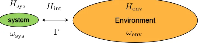
FIG. 1: General framework for an open quantum system: A small quantum system interacts with its environment, leading to a combination of coherent and dissipative dynamics for the small system. In quantum optics, and atomic, molecular, and optical (AMO) systems more generally, the resulting dynamics can both be microscopically well understood, as well as controlled to engineer dynamics or specific quantum states. This involves a separation of energy and frequency scales, where the energy and frequency scales of the small system that are directly coupled to the environment (ωsys) and the relaxation rates for relevant correlation functions in the environment (ωenv) are

much larger than the frequency scales of dynamics induced by the coupling (Γ).

[27, 28]. The study of open quantum systems also has importance in cosmology [29], and quantum-optical approaches have recently been applied to treat pion decay in high-energy physics [30, 31].

While many studies seek to characterise and reduce the destruction of quantum coherence in an open system, a key guiding aim in quantum optics over the last thirty years has been the use of controlled coupling to the environment to control and manipulate quantum coherence with high precision. This includes manipulating the environment in such a way as to drive the system into desired quantum states, increasing quantum coherence in the sample. In the laboratory, this philosophy began with optical pumping in atomic physics [32, 33], whereby using laser driving and spontaneous emission processes, atoms can be driven into a single atomic state with extraordinarily high fidelities approaching 100%. This has lead on to techniques for laser cooling of trapped ions [20, 34, 35] and of atomic and molecular samples [36], which has allowed the production of atomic gases with temperatures of the order of 1 µK. This, in turn, set the stage for realising Bose-Einstein condensation [37–39] and degenerate Fermi gases [40, 41], as well as providing a level of high-precision control necessary for quantum computing with trapped ions [17, 20, 42]. Such driving processes, making use of the coupling of the system to its environment, have been extended to algorithmic cooling in Nuclear Magnetic Resonance (NMR) systems [43, 44], and are recently being applied to cool the motional modes of macroscopic oscillators to near their quantum ground state [45]. A detailed understanding of the back-action on the quantum state of the system from coupling to the environment has also been useful in the context of high-fidelity state detection (e.g., in electron shelving [46–51]), or in quantum feedback [52–56], and have also been exploited for control over atoms and photons in Cavity QED [57, 58].

This high level of control is possible because in quantum optics several key approximations can often be made regarding the coupling of a system to its environment, which in combination make the control of this coupling both tractable theoretically and feasible experimentally. This includes the fact that the dynamics are often Markovian (i.e., the environment relaxes rapidly to an equilibrium state and on relevant timescales has no memory of previous interactions with the system), and that the system-environment coupling is typically weak compared with relevant system and environment energy scales. The possibility of making such approximations has resulted in the development of several complementary formalisms, including quantum Langevin equations [59–63], quantum master equations [2, 59, 64, 65], and continuous measurement theory [2, 52]. These techniques and related ideas have been applied extensively over the last thirty years to a variety of single-particle and few-particle quantum systems, especially in the context of atomic, molecular, and optical (AMO) experiments. Techniques such as quantum master equations in Lindblad form [2] are sometimes applied in other contexts, especially in a range of solid-state systems. However, many solid-state systems are dominated by non-Markovian aspects of their dissipative dynamics [1], which are consequently not captured by this form. This is in strong contrast to the AMO/quantum optics context, where the approximations involved in deriving these equations are typically good to many orders of magnitude.

the dissipative process being described by a modification to the Hamiltonian, combined with quantum jumps - sudden changes in the state that take place at particular times. By taking an appropriate stochastic average over the times and type of quantum jumps, expectation values for the system propagated under the master equation can be faithfully and efficiently reconstructed within well-controlled statistical errors. This technique is particularly appealing, because when combined with continuous measurement theory, it can also help to give a physical intuition into the workings of the dissipative process.

B. Open many-body quantum systems in a AMO context

Over the last decade and a half, AMO systems (cold atoms and molecules, as well as trapped ions and photons) have been increasingly used to study strongly-interacting many-body systems. This has reached a level where these systems can be used to engineer microscopic Hamiltonians for the purposes of quantum simulation [6, 70–76]. As a result, it has become important to explore the application of existing experimental techniques and theoretical formalisms from quantum optics in this new many-body context. Particularly strong motivation in this respect has come from the desire to engineer especially interesting many-body states, which often require very low temperatures (or entropies) in the system. An example of this are low-temperature states of the fermionic Hubbard model, which can be engineered in optical lattices [75, 76]. Many sensitive states in this model arise because of dynamics based on superexchange interactions, which arise in perturbation theory and can be very small in optical lattice experiments. A key current target of optical lattice experiments is the realisation of magnetic order driven by such interactions [77–80], with eventual goals to realise more complex spin physics or even pairing and superfluidity of repulsively interacting fermions [75]. For these and other fragile states, understanding dissipative dynamics in the many-body system is then necessary both to control heating processes, and to provide new means to drive the systems to lower temperatures.

Such studies are particularly facilitated by the fact that many of the same approximations that are made in describing open few-particle systems in quantum optics can also be made in these AMO many-body systems. This means both that the physics of open systems as they appear in quantum optics can be investigated in a wholly new context, and that mathematical techniques such as master equations and quantum Langevin equations, as well as numerical techniques such as quantum trajectory methods can be immediately applied to these systems in a way that faithfully represents the microscopic physics.

This has already lead to many important developments. Some of these have direct practical importance in the experiments - e.g., in order to cool many-body systems to the temperatures required to realise important many-body physics [80], it has become important to understand decoherence in a many-body context in order to characterise the related heating processes [81–86]. Other studies have involved funda-mentally different approaches to state preparation, including studies of how to use controlled dissipation to produce new cooling methods [87–91], or to drive the system into desired many-body states - including Bose-Einstein condensates (BECs) or metastable states such asη pairs [92, 93], paired states [94–98], or even states with topological order [99, 100]. Dissipation can also play a key role in suppressing two-body [23, 101–103] and three-body [104–106] loss processes via a continuous quantum Zeno effect, enabling the production of interesting many-body states requiring effective three-body interactions [104, 107–121], and similar effects are seen in locally induced single-particle losses in cold gases [122–124]. Such effects can also be used to manipulate or protect states in quantum computations [125, 126] and quantum memories [127], as well as to prepare entangled states dissipatively [128–130], or realise specific quantum gates for group-II atoms [131, 132]. It is also possible to generate spin-squeezed states using collisional loss in fermions [133] or collisions with background gases [134], as well as to protect states during adiabatic state preparation [135].

C. Purpose and outline of this review

As is clear from the previous section, this area of research, combining ideas and techniques from quantum optics with strongly interacting many-body systems, has developed dramatically in the last few years. Control over dissipation promises many new tools to prepare interesting and important many-body states, and to investigate models in quantum simulators that are inaccessible to current methods.

In this review, we set about facilitating discussion between the AMO and many-body communities by introducing open many-body systems as they are understood in the AMO context. We will focus on real-time dynamics, especially of open quantum system out of thermal equilibrium. We will also build our discussion around the use of quantum trajectory techniques, which provide a numerical method for detailing with dissipative dynamics, and also together with continuous measurement theory, provide a way to understand the dynamics for this class of open AMO quantum systems. We discuss the numerical imple-mentation of quantum trajectories for many-body systems, and address a series of examples highlighting interesting physics and important tools that are already being explored in these dissipative many-body systems.

The review is structured as follows – we begin with a brief introduction to open quantum systems as they are discussed in quantum optics, noting the key approximations that can be made for many open AMO systems, and introducing notation. We then give an introduction to the quantum trajectories method and its physical interpretation, as well as its integration with time-dependent methods for many-body systems, especially the time-dependent Density Matrix Renormalisation Group (t-DMRG). We then introduce several examples of open many-body AMO systems, including light scattering from strongly interacting atoms in an optical lattice, collisional two-body and three-body losses as well as loss processes with single atoms, and quantum state preparation by reservoir engineering – including methods to drive systems dissipatively into states with important many-body character. We finally return to further details of the physical interpretation of quantum trajectories by briefly introducing continuous measurement theory, before finishing with an outlook and summary.

II. OPEN QUANTUM SYSTEMS IN QUANTUM OPTICS

Throughout this review, we will work in the framework of a quantum optics description of open quantum systems. Open quantum systems have been regularly discussed in many areas of physics, but the AMO systems that are studied in quantum optics often enable a series of approximations that allow specific types of understanding and control over the dynamics. In this section we introduce the concept of an open system, and the key approximations that lead to simplified descriptions of system dynamics. We then introduce a key example of those descriptions, specifically the Lindblad form of the master equation.

A. General framework

The general framework for an open quantum system is sketched in Fig. 1 [1, 2]. We consider a small quantum system1_{, which is coupled to a largeenvironment, which can also be thought of as areservoir.}

This is a similar relationship to the heat bath and the system in the canonical ensemble of statistical mechanics, and for this reason the environment is also referred to as the “bath” in some literature.

In this setup, the Hamiltonian for the total system, including both the system and its environment, consists of three parts,

Htotal=Hsys+Henv+Hint. (1)

HereHsysis the system Hamiltonian, describing the coherent dynamics of the system degrees of freedom

alone, in the absence of any coupling to the reservoir. In quantum optics, this is often a two-level system (e.g., an atom, a spin, or two states of a Cooper pair box), in which case we typically might haveHsys=

1 _{In a many-body context, a “small” quantum system might be relatively large and complex – it should just be very}

~ωsysσz, whereωsysis a system frequency scale, andσz is a Pauli operator for a two-level system. Another

common system is to have a harmonic oscillator (e.g., a single mode of an optical or microwave cavity, or a single motional mode of a mechanical oscillator), with system HamiltonianHsys =~ωsysa†_hoaho, where aho is a lowering operator for the harmonic oscillator. The degrees of freedom for the environment and

their dynamics are described by the hamiltonian Henv, and the interaction between the system and the

reservoir is described by the hamiltonianHint.

In quantum optical systems the reservoir usually consists of a set of bosonic modes, so that

Hres=

X

l Z ∞

0

dω~ω b†l(ω)bl(ω), (2)

where bl(ω) is a bosonic annihilation operator for a mode of frequency ω. The indexl is convenient for

describing multiple discrete modes at a given frequency, e.g., in the case that these are the modes of an external radiation field,l can play the role of a polarisation index. These operators obey the commutation relation [bl(ω), b†l(ω0)] = δ(ω−ω0)δll0, where δ(ω) denotes a Dirac delta function and δ_ll0 a Kronecker

delta. Note that in general, a reservoir can have a frequency-dependent density of modes g(ω), which we have assumed for notational convenience is constant in frequency. Below when we make a Markov approximation for the dynamics, we will assume that this density of modes is slowly varying over the frequencies at which the system couples to the reservoir.

The interaction HamiltonianHint analogously takes a typical form

Hint = −i~X

l Z ∞

0

dω κl(ω) x+l +x−l h

bl(ω)−b†l(ω) i

(3)

≈ −i~

X

l Z ∞

0

dω κl(ω) h

x+_l bl(ω)−x−_l b†_l(ω) i

, (4)

wherex±_l is a system operator, andκ(ω) specifies the coupling strength. In connection with the two-level systems listed above, for a two-level system, we might have x−_l = σ−_{, the spin lowering operator, and} x+_l = σ+_{, the spin raising operator. In the case that the system is a Harmonic oscillator, we would}

typically havex−_l =aho. In the second line of this expression, we have explicitly applied a rotating wave

approximation, which we will now discuss.

B. Key approximations in AMO systems

A key to the microscopic understanding and control that we have of open AMO quantum systems is the fact that we can usually make three approximations in describing the interaction between the system and the reservoir that are difficult to make in other systems [2]:

1.The rotating wave approximation - In the approximate form eq. (4) of the interaction Hamiltonian we gave above, we neglected energy non-conserving terms of the form x+_l b†_l(ω) and x−_l bl(ω). In

general, such terms will arise physically in the couplings, and will be of the same order as the energy conserving terms. However, if we transform these operators into a frame rotating with the system and bath frequencies (an interaction picture where the dynamics due to Hsys and Henv are

incorporated in the time dependence of the operators), we see that the energy-conserving terms will be explicitly time-independent, whereas these energy non-conserving terms will be explicitly time-dependent, rotating at twice the typical frequency scale ωsys. This is shown explicitly below

in eq. (A2) in section A 1. In the case that this frequency scale is much larger than the important frequency scales for system dynamics (or the inverse of the timescales for which we wish to compute the dynamics), the effects of these energy non-conserving terms will average to zero over the relevant dynamical timescales for the system, and so we can neglect their effects in describing the dynamics.

2.The Born approximation - We also make the approximation that the frequency scales associated with dynamics induced by the system-environment coupling is small in scale compared with the relevant system and environment dynamical frequency scales. That is, if the frequency scalesωsysat

!

a)

b)

!

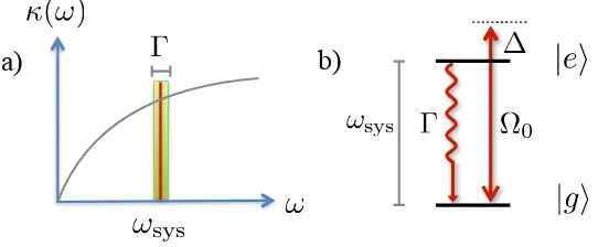
FIG. 2: (a) Coupling constant as a function of frequency, κ(ω), illustrating a slowly varying coupling strength around the central system frequencyωsys. This is a key to several of the approximations made for open quantum

systems in quantum optics. (b) Comparison of the scales for a two-level system. The system frequency is the optical frequency,ωsys, associated with the energy difference between the ground and excited levels. In order to make the

standard approximations, we require the timescale for the decay of the excited state, Γ−1, i.e., the timescale for the dynamics induced by coupling to the environment, to be much longer than the optical timescale associated with the transition, or in freqeuncy units, Γ−1 ωsys−1. We also work in a limit where any remaining system

dynamics are associated with much smaller frequency scales. In this case, the coupling strength Ω0, associated

with the frequency of Rabi oscillations between the states when they are coupled strongly on resonance, as well as the frequency of detuning from resonance ∆, satisfy Ω0,∆ωsys.

3.The Markov approximation - We assume that the system-environment coupling is frequency/time-independent over short timescales, and that the environment returns rapidly to equilibrium in a manner essentially unaffected by its coupling to the system, so that the environment is unchanged in time, and the dynamics of the system are not affected by its coupling to the environment at earlier times, i.e., the time evolution of the system does not depend on the history of the system.

Each of these three approximations are normally exceptionally well justified, with the neglected terms in equations of motion being many orders of magnitude smaller than those that are retained. This results from the existence of a large frequency/energy scale that dominates all other such scales in the system dynamics described by Hsys, and in the system-environment interaction Hint. Specifically, we usually

have a situation where [Hsys, x±_l ] ≈ ±~ωlx±_l , and the frequencies ωl, which are all of the order of some

system frequencyωsys, (1) dominate any other processes present in the system dynamics, and (2) are much

larger than the frequency scales of dynamics induced by coupling to the reservoir, Γ. The first of these two conditions allows us to make rotating wave approximations in the interaction Hamiltonian, without which we could not make the Markov approximation. The second of these allows us to make the Born approximation.

The Markov approximation can be physically interpreted in two parts: it implies firstly that the system-environment coupling should be independent of frequency, to remove any back-action of the system-environment on the system that is not local in time, and secondly, that any correlation functions in the reservoir should retain no long-term memory of the interaction with the system. The first of these two pieces is again justified by the large frequency scale for the energy being transferred between the system and the reservoir relative to the effective coupling strength. As depicted in Fig. 2, the system and environment couple in a range of frequencies that is of the order of the effective coupling strength, Γ, and if Γωsys, then the

variation in coupling strengthκ(ω) over the range of frequencies where the modes couple significantly to the system is very small. For a single indexl, we can writeκ(ω)_≈pΓ/(2π). Note that we implicitly made this assumption for the density of modes in the reservoir g(ω) when we didn’t include such a density of modes in eqs. (2) and (4) above. The second requirement depends on the physical details of the reservoir, and justifying this part of the approximation usually requires comparing the typical coupling timescales Γ−1_{with environment relaxation timescalesω}−1

env, which are in general different toωsys−1. However, for many

typical cases, we also find thatωenv∼ωsys.

In the case of decaying two-level atoms, or loss of photons from an optical cavity, these timescales are both related to the relevant optical frequency. On a physical level, when a two-level atom decays and emits a photon of wavelengthλoptand frequencyωopt, then the relevant system timescaleωsys−1=ω−opt1, and

we have a requirement that the decay time, which is the relevant system-environment coupling timescale Γ−1_{, is much longer than ω}−1

the photon to propagate away from the atom within the photon wavelengthλis also of the order 1/ωopt.

In that sense, the single frequencyωopt is the large frequency scale for each of the three approximations.

The ratio of this frequency scale to Γ is, for typical optical systems _∼ 1015_/108 _{= 10}7_{, so that the}

approximations made here are good to many orders of magnitude.

C. Master Equation

The approximations given above make it possible to derive an equation of motion for the behaviour of the system alone in the presence of the dissipation due to coupling to the environment. Because of the combination of dissipative and coherent dynamics, this is expressed in terms of the density operator ρ describing the state of thesystem, which can be defined based on the total density operator for the system and the environmentρtotalasρ= Trenv{ρtotal}, where the trace is taken over the environment degrees of

freedom. There are many routes to derive such an equation of motion (see, e.g., [1, 2, 59, 64, 65]), one of which is outlined in appendix A, via a continuous measurement formalism.

The resulting markovianmaster equation takes a Lindblad form [172] (see, e.g., [2, 59, 65])

˙ ρ = −i

~[H, ρ]− 1 2

X

m

γm˜c†m˜cmρ+ρc˜†mc˜m−2˜cmρc˜†m

. (5)

Here, H is the remaining system Hamiltonian, after the frequency scale ωsys of the coupling between the

system and the environment has been transformed away. For a two-level system, this is a Hamiltonian describing the coupling between levels and a detuning in the rotating frame (see section III F 1 below), i.e., in an interaction picture we we transform the operators so that we make the dominant coupling terms in the Hamiltonian time-independent. The operators ˜cm are sometimes called Lindblad operators (or

jump operators, as described below), and describe dissipative dynamics (including decoherence and loss processes) that occur at characteristic ratesγm.

Note that the ˜cmare all system operators, and the time-dependence of the environment does not appear

in this equation. For the interaction Hamiltonian in Eq. (4), if we assume that all of the reservoir modes that couple to the system are unoccupied, we will have ˜cl=x−l . One example of ˜cmwould be a transition

operatorσ−from an excited state to a ground state in the two-level system depicted in Fig. 2b, describing spontaneous emissions, and further examples are given below in sections III D, III F and V. We also note at this point that in general, the ˜cmare non-Hermitian, although they can always be interpreted as resulting

from continuous measurement of Hermitian operators acting only on the environment, as discussed in appendix A. In the case that all ˜cmare Hermitian, we can think of this master equation as representing

a continuous measurement of the system operatorscm.

The general form in eq. (5) also demonstrates explicitly the trace-preserving property of the master equation (Tr_{ρ˙_}= 0). This form of dissipative dynamics is sometimes used as a toy model for dissipation because of its relatively simple interpretation. In the AMO / quantum optics context, it is particularly im-portant because it describes the microscopic behaviour under the well-controlled approximations described in section II B.

In order to reduce the notational complexity, we will combine the rate coefficients with the operators in the formcm=√γmc˜m, and we will also equate energy and frequency scales setting ~≡1, to obtain

˙

ρ = −i[H, ρ]−1₂X

m

c†mcmρ+ρcm† cm−2cmρc†m

,

Note that we can also express this in the convenient alternative form

˙

ρ = ₋i(Heffρ−ρHeff† ) +

X

m

cmρc†m, (6)

where we refer to

Heff =H−

i 2

X

m c†mcm

as the effective Hamiltonian for the dissipative system. in this form, the termP_mcmρc†m is often called

effective Hamiltonian, placing it in other states. For a two level system with decay from an excited state to the ground state, one may think of the non-Hermitian part as removing amplitude from the excited state, and the recycling term as reinstating this in the ground state (see the many-body examples for a more detailed discussion of this).

For some simple systems, master equations can be solved analytically, to obtain expectation values of a given physical observableAat particular times,hA(t)i= Tr{Aρ(t)}or also two-time correlation functions of the form_hA(t+τ)B(t)_i. In the next section we will discuss how the dynamics described by the master equation can be both computed and physically interpreted using quantum trajectories techniques. We then give some specific examples of small physical systems described by master equations. In the following two sections, we then discuss how master equations of the form eq. (6) describing many-body systems can be solved by combining quantum trajectories techniques with many-body numerical methods, and then discuss a number of examples of recent work on such physical systems.

III. QUANTUM TRAJECTORIES

Quantum trajectory techniques were developed in Quantum Optics in the early 1990s [3, 66–69, 173] as a means of numerically simulating dissipative dynamics, and can be applied to any system where the time evolution of the density operator is described via a master equation (in Lindblad form). These techniques involve rewriting the master equation as a stochastic average over individualtrajectories, which can be evolved in time numerically as pure states. These techniques avoid the need to propagate a full density matrix in time (which is often numerically prohibitive), and replace this complexity with stochastic sampling. The key advantage this gives is that if the Hilbert space has dimensionNH, then propagating

the density matrix means propagating an object of sizeN2

H, whereas stochastic sampling of states requires

propagation of state vectors of size NH only. Naturally, the penalty that is paid is the need to collect

many samples for small statistical errors, and it is important that the number of samples required remains smaller than the size of the Hilbert space in order to make this efficient.

In quantum optics, these techniques were developed in parallel by a number of groups, as they arose out of studies of different open-quantum system phenomena. The versions of these techniques that most closely resemble what we present here were developed by Dalibard, Castin and Mølmer [67, 68] as a Monte Carlo method for simulation of laser cooling; by Dum et al. [69, 173], arising from studies of continuous measurement; by Carmichael [3], in studying of the generation of non-classical states of light; and by Hegerfeldt and Wilser [174], in modelling a single radiating atom. The term quantum trajectories was coined by Carmichael, whereas the other approaches were referred to as either aquantum jump approach, or theMonte Carlo wavefunction method. This later term should not be confused with so-calledquantum Monte Carlo techniques - the Monte Carlo treatment performed here is classical, in the sense that there is no coherent sum of amplitudes involved in evaluating expectation values from the samples we obtain. Mathematically, all of these approaches are essentially equivalent, but there are differences in the numerical implementations.

In quantum optics these methods have been applied to a wide variety of problems, including laser cooling [68, 175–177] and coherent population trapping [178], the behaviour of cascaded quantum systems [179–181], the continuous quantum Zeno effect [182–184], two-photon processes [185], decoherence in atom-field interactions [186], description of quantum non-demolition measurements [187] and decoherence in the atom-optics kicked rotor [188–191]. For further examples, see the review by Plenio and Knight [66] and references therein. Note that complementary stochastic approaches were developed at the same time, especially by Gisin and his collaborators [192–194]. These and other related quantum state diffusion approaches [195, 196] involve continuous stochastic processes, but can be directly related back to the quantum trajectories formalism by considering homodyne detection of the output of a quantum system (see, e.g.,[3, 197]).

A. Stochastic averages and quantum mechanical expectation values

In determining expectation values of a particular operatorAbelow, we will often have to take both the quantum mechanical expectation value and a stochastic average. To determine the expectation value of a quantity from a system density operatorρ, we compute hAi= Tr{Aρ}. If we can expand the density operator in terms of pure states|ζliasρ=P_lpl|ζlihζl|, then we can also expand

hAi= Tr{Aρ}=X

l

plhζl|A|ζli ≡ X

l

plAl≡Al. (7)

The expression_hζi|A|ζiiis a quantum mechanical expectation value, and the weighted sum over l gives

a statistical or stochastic average over the values in the sum for each state _|ζli, Al = hζl|A|ζli. Below,

we will denote the total expectation value of an operator with angle brackets_hA_i as we do here. Where we explicitly want to denote a stochastic or statistical average only, we will either use an overlineAl or a

subscript on the angle brackets,hAlis.

B. First-order Monte Carlo wavefunction method

The simplest form of the quantum trajectory method involves expanding the master equation to first order in a time step δt, and was first described in this form by Dalibard et al. [67] and Dum et al. [69]. It involves the evolution of individual trajectories_|φ(t)_i, over which we average values of observables.

For a single trajectory, the initial state_|φ(t= 0)_ishould be sampled from the density operator at time t= 0,ρ(t= 0). For some systems, ρ(t= 0) may be a pure state, and this is the case for a number of our many-body examples. In that case, the initial state is always the same state,ρ(t= 0) =_|φ(t= 0)_ihφ(t= 0)|. Once we have an initial state, we propagate forward in time, making use of the following procedure in each time step:

1. Taking the state at the beginning of the time step,|φ(t)i, we first compute the evolution under the effective Hamiltonian. This will give us one candidate for the new state at time t+δt,

|φ(1)_(t+δt)

i= (1₋iHeffδt)|φ(t)i, (8)

and we compute the norm of the corresponding state, which will be less than one because Heff is

non-Hermitian:

hφ(1)(t+δt)_|φ(1)(t+δt)_i = _hφ(t)_|1 + iH_eff† δt(1₋iHeffδt)|φ(t)i (9)

= 1−δp. (10)

Here, we can consider δp as arising from different potential decay channels, corresponding to the action of different Lindblad operators cm,

δp = δt_hφ(t)_|i(Heff −Heff† )|φ(t)i (11)

= δtX m

hφ(t)|cm† cm|φ(t)i ≡ X

m

δpm. (12)

We can effectively interpretδpmas the probability that the action described by the operatorcmwill

occur during this particular time step.

2. Then, we choose the propagated state stochastically in the following manner. We would like to assign probabilities to different outcomes so that:

• With probability 1−δp

|φ(t+δt)i= |φ

(1)_(t+δt)i

√

1−δp (13)

• With probabilityδp

|φ(t+δt)_i= pcm|φ(t)i δpm/δt

where we choose oneparticular m, which is taken from all of the possiblemwith probability

Πm=δpm/δp (15)

In a practical numerical calculation, this action requires drawing a uniform random number r1

between 0 and 1, and comparing it with δp. Ifr1 > δp, then no jump occurs, and the first option

arrising from propagation under Heff, i.e., |φ(t+δt)i ∝ |φ(1)(t+δt)i is chosen. Ifr1 < δp, then a

jump occurs, and we must choose the particularcmoperator to apply. We therefore associate eachm

with an interval of real numbers, with the size of the interval being proportional toδpm. Normalising

the total interval length to one so that every m corresponds uniquely to a range between 0 and 1, we then choose a second random numberr2, also uniformly distributed between 0 and 1, and choose

the associatedcmfor which the assigned interval containsr2.

In order to see that this stochastic propagation is equivalent to the master equation, we can form the density operator,

σ(t) =_|φ(t)_ihφ(t)_|. (16)

From the prescription above, the propagation of this density operator in a given step is:

σ(t+δt) = (1−δp)|φ

(1)_(t+δt)i

√ 1−δp

hφ(1)_(t+δt)|

√

1−δp +δp X

m

Πmpcm|φ(t)i δpm/δt

hφ(t)|c†m p

δpm/δt

, (17)

whereX for anyX denotes a statistical average over trajectories, as opposed to the quantum mechanical expectation values or mathematically exact averages, which we will denotehXi. Rewriting the terms from the above definitions, we obtain

σ(t+δt) = σ(t)₋iδt(Heffσ(t)−σ(t)Heff† ) +δt

X

m

cmσ(t)c†m, (18)

which holds whetherσ(t) corresponds to a pure state or to a mixed state. In this way, we see that taking a stochastic average over trajectories is equivalent to the master equation

˙

ρ=−i(Heffρ−ρHeff† ) +

X

m

cmρc†m. (19)

Note that the equivalence between the master equation and the quantum trajectories formulation doesn’t require a particular choice of δt. In particular,δtcan be chosen to be small in evaluating this evolution. Naturally, choosing very largeδtwould strongly compromise the accuracy of the method when propagating the state in time. In the subsection III E, we will deal with how to improve upon this first-order method numerically.

1. Computing single-time expectation values

In order to compute a particular quantity at time t, i.e., _hA_it = Tr{Aρ(t)}, we simply compute the

expectation value of Afor each of our stochastically propagated trajectories, _hφ(t)_|A_|φ(t)_i, and take the average of this quantity over all of the trajectories,

hA_it≈ hφ(t)|A|φ(t)i. (20)

Provided our random number generators are well behaved, the trajectories are statistically independent, allowing for simple estimate of statistical errors in the computation ofhAit, as discussed in section III C.

2. Computing two-time correlation functions

correlation functions from a master equation, we typically apply the quantum regression theorem [2, 200], which can be applied generally to an operatorXij=|iihj|, where|iiand|jibelong to an orthonormal set

of basis states for the Hilbert space. If we writeCij(t, τ) =hXij(t+τ)B(t)i, then we note thatCij(t,0)

are one-time averages that can be calculated directly from the density matrix at a single time, and theτ dependence can be computed as

∂Cij

∂τ (t, τ) = X

kl

MijklCkl(t, τ), (21)

where theMijklare the same matrix elements that appear in the equation of motion for one-time averages

[2, 200]

d_hXij(t)i dt =

X

kl

MijklhXkl(t)i. (22)

To reproduce these values from quantum trajectories, we follow a simple procedure [66, 68]. We propa-gate a sample trajectory to timet, and then generate four helper states:

|χR_±(0)i = q1 µR

±

(1±B)|φ(t)i, (23)

|χI

±(0)i = 1

q µI

±

(1_±iB)_|φ(t)_i, (24)

whereµR

±andµI±normalise the resulting helper states. We then evolve each of these four states using the quantum trajectories procedure, and compute the correlation functions

cR_±(τ) =hχR_±(τ)|A|χR_±(τ)i, (25) cI_±(τ) =hχI_±(τ)|A|χI_±(τ)i. (26)

We can then reconstruct a sample for

C(t, τ) = 1 4

µR+cR+(τ)−µR−cR−(τ)−iµI+cI+(τ) + iµI−cI−(τ)

, (27)

and average this over both the evolution up to timet and the propagation of helper states to timeτ.

C. Statistical Errors and convergence

1. Estimating statistical errors

Using the above procedure or generalisations that are higher-order in the timestepδt(see section III E), we generateN sample trajectories. Under the assumption that the random numbers used in the numerical implementation are statistically random and uncorrelated2, these trajectories are statistically independent, and we can estimate the correct meanhXiof any operator of interest ˆX as

X(t) = 1 N

X

i Xi≡

1 N

X

i

hφi(t)|Xˆ|φi(t)i. (28)

The central limit theorem implies that for sufficiently largeN, the probability distribution forX will be well approximated by a Gaussian distribution with mean hXi. The statistical error in this mean is the

2 _{See, e.g., Ref. [201] for a general discussion of random number generators. For typical calculations, only a few tens of}

standard deviation of that distribution, which in turn can be estimated based on the variance of the values Xi in the following way. Denoting a statistical average as h. . .is, we consider

Var[X] = D X_{− h}X_is

2E

s= *

1 N

N X

i=1

Xi !2

−2X_hX_is+hXi2s +

s

= 1

N2

N X

i=1

N X

j=1

hXiXji_s− hXi2s=

1 N2

N X

i=1

X2

i

s+ N₋1

N hXi

2

s− hXi2s

= 1

N(hX

2

is− hXi2s) =

1

NVar[X].

(29)

In deriving this standard result, we use both the independence of the trajectories _hXiXj6=iis =

hXiishXj6=iis, and the replacement that hXis = hXis, i.e., the variance written in the last line is the

true variance of the distribution forX. As a result, it can be shown (see, e.g., Ref. [201]) that we should use the approximator

Var[X]≈

PN

i=1(Xi−X)2

N₋1 , (30) if we would like to estimate this based on the samples we obtain in the calculation.

In this sense, we can always calculate the statistical errorσAin our estimate of a quantityhAiby taking

theestimate of the population standard deviation∆Afrom ourN samples, anddividing by√N,

σA=

∆A √

N. (31)

How many trajectories we will require for good convergence will depend both on the details of the dynamics and on the quantity being calculated. For variables with non-zero mean, we would typically like to have σA/hAi 1, which implies that

√

N ∆A/_hA_i. As the sample estimate overestimates the population standard deviation (see e.g., [68]), we can consider the sample estimate for the standard deviation ∆Ahere.

2. Global quantities vs. local quantities

In Mølmer et al. [68], there is a discussion of the different number of trajectories required for global quantities vs. local quantities to be straight-forwardly estimated. This is done for single-particle systems in a Hilbert space dimensionNH.

Forglobal quantities such as the total energyAG =Etot, there is usually a fixed relationship between

the estimate ∆AG andhAGithat is independent of the dimension of the Hilbert spaceNH. For example,

in the Brownian motion of a particle thermalised with a reservoir at temperature T, we would expect hAGi ≈(3/2)kBT, wherekB is the Boltzmann constant, and ∆AG≈

p

3/2kBT. The requirement on the

number of trajectories is then simplyN 1, and we should expect that the relative error is well estimated by 1/√N (so that for 10% relative statistical error, we would requireN ∼100 trajectories. These same arguments apply to many-particle systems, we also expect global averages involving all of the particles in a system (or all of the spins or lattice sites in a spin or lattice system) to be efficiently treatable with quantum trajectories methods.

For local quantities in a single-particle calculation, the opposite is true. If we try to determine the population of a given eigenstate (of the Hamiltonian, or of the momentum operator), then we expect that in a Hilbert space of dimension NH, our local quantities AL and their statistical variance will behave

as _hALi ∼ 1/NH and σA2 ∼ 1/NH. As a result, we see that we require N NH for good statistical

convergence, and there is no advantage in using a quantum trajectories technique over direct integration of the master equation.

However, forlocal quantities in many-body systems, the situation is not as clear-cut. If we attempt to compute the population of a given many-body eigenstate out ofNH possible many-body eigenstates, then

as the size of the system, L, whereas for large systems with fixed particle density, NH ∝exp(L). As a

result, quantities such as the local density on one site in a lattice of L sites, or individual elements of a single-particle density matrix on such a lattice will tend to scale as _hASi ∼ 1/L and σA2 ∼1/L. We

therefore requireN L for good statistical convergence, and notN NH. Although this will require

more trajectories for small relative statistical error than in the case of global quantities (by a factor of√L), there are often still large advantages in using quantum trajectory techniques to calculate these quantities when the size of the Hilbert spaceNH becomes large.

We will discuss this again below, when we give two illustrative examples for the use of quantum tra-jectories in section III F. Specifically, in section III F 2, we treat the dephasing of hard-core bosons on a lattice, and consider calculation of the total energy, local single-particle correlations, and local densities using quantum trajectory techniques.

D. Physical interpretation

One of the greatest strengths of the quantum trajectories approach to dissipative systems, but also one of the most subtle points in its usage, is that it gives us a simple physical interpretation for the physics induced by the environment on the system. The method is also known as the method ofquantum jumps, and the Lindblad operatorscmare also calledjump operators, inviting the picture of a system that evolves

under the non-Hermitian effective HamiltonianHeff and then undergoesquantum jumps at certain points

in time. The master equation is then an appropriately weighted stochastic average over all of the different times at which the jumps could occur, and all of the different types of jumps that can occur.

To see this working in practice, consider a two-level system like that depicted in Fig. 2b. If we drive the system, coupling the excited and ground states (_|e_iand_|g_i) respectively with an effective Rabi frequency Ω0and a detuning ∆, then the system will undergo coherent dynamics, interrupted at particular times by

spontaneous emission events, which return the atom to the ground state_|g_i, due to the action of a jump operator c =√Γ_|g_ihe_|. If photons can be scattered in multiple directions, then the different directions constitute different channelscm, and we can average over the probability distribution of emission directions.

Note that this is presented carefully below in section V B. The stochastically chosen times for the jumps are the times at which spontaneous emissions occur, and stochastically sampling differentmvalues amounts to a stochastic sampling of the direction in which the photon is emitted.

This is a very appealing intuitive picture of the dynamics, and connects strongly with an intuition of what would happen if we are actually able to measure the environment. Indeed, quantum trajectories techniques were originally developed by certain groups from studies of photon counting [174], or continuous measurement [69]. If we are able to make perfect measurements and we see a photon appear in the time window δt, then we know that a jump has occurred, and that the state of the atom should be projected on the ground state. On the other hand, if we know that no jump has occurred, then the corresponding evolution of the system is an evolution under the effective HamiltonianHeff. Already here, we see a key

piece of physics that will recur multiple times: knowing that no jump has occurred means that we gain information about the system, just as knowing that a jump has occurred gives us information that the atom is projected into the ground state.

To see this in a simple example, consider preparing the system in a state _|ψ(t)_i =α_|g_i+β_|e_i, where α and β are complex coefficients, and set Ω0 = ∆ = 0. We can then ask what we expect to happen

in a single step, depending on whether we observe a spontaneously emitted photon or not. As we are not concerned about the motion of the atom, or therefore about the direction of spontaneously emitted photons, we can consider a single jump operator c = √Γ_|g_ihe_|, and an effective Hamiltonian which is simplyHeff =−i(Γ/2)|eihe|. If a jump occurs in a time stepδt, then the state after this jump is

|ψ(t+δt)i= c|ψ(t)i

kc|ψ(t)ik =|gi. (32)

So if there is a spontaneous emission, then the state is projected onto the ground state, as expected. Consider now what happens if no jump occurs: We then evolve the state as

|ψ(t+δt)_i= exp(−iHeffδt)|ψ(t)i kexp(−iHeffδt)|ψ(t)ik

= α|gi+βe−

Γδt/2

|e_i kα|gi+βe−Γδt/2_|eik =

α_|g_i+βe−Γδt/2

|e_i p

|α|2_+|β|2_e−Γδt. (33)

emitted photon, we have gained the knowledge that the system is somewhat more likely to be in the ground state than in the excited state, and this gain in knowledge is reflected in the relative probabilities for occupation of these states at timet+δtrelative to timet. Thus, the dynamics are affected by coupling to the environment even in the absence of actual spontaneously emitted photons.

There are two important cautions to over-interpreting this intuitive physical picture. Firstly, the master equation can typically be expanded in different sets of jump operators. If there exists a unitary transfor-mationT in the Hilbert space of the system such that for the dissipative part of the master equation

Lρ=₋1 2

X

m

c†mcmρ+ρcm† cm−2cmρc†m

, (34)

the operatorT satisfies the condition

T[Lρ]T† =L T ρT†, (35)

then we can rewrite each jump operator cm such that we obtain new operators dm=T†cmT, and show

[68] that

Lρ=₋1 2

X

m

d†mdmρ+ρdm† dm−2dmρd†m

. (36)

In this sense, the operatorsdm are equally good choices for the jumps as the operators cm. In general,

for the application of quantum trajectories as a numerical method, we should simply choose the jump operators that provide most rapid convergence of sampling. This has been investigated in a number of contexts [68, 203–206], including quantum feedback [207]. However, to ascribe physical meaning to an individual trajectory it is important to be able to associate the specific jumps with measurable properties of the environment after the jump. This detector dependence should even produce measurable differences under certain conditions [208].

In addition, ascribing a pure state to the system as a function of time implies knowledge of measure-ment results from the environmeasure-ment. Although each trajectory implies a particular physical picture of the dissipation, it is the average over trajectories that properly specifies our knowledge of the system if we do not measure the environment. At the same time, there are sometimes means to make a measurement on the system and infer the measurement result for the environment. A simple case of this type of postselec-tion appears when the dissipative process we deal with is dominated by particle loss, as we will treat in section V C below. There, if we know that no particles are lost by making a measurement at the end of a dynamical process, then we can project the state of the system on the state simply evolved under the effective HamiltonianHeff, as this is an equivalent mechanism to measure that no jumps occurred during

the evolution.

In order to address how the approximations that we can make in AMO systems give rise to the behaviour exhibited by the system, we will re-derive the quantum trajectory approach in appendix A. There we will make explicit this connection between measurement of the environment and inference of the state of the system.

E. Alternate formulation for higher-order integration in time

The downside of the method presented in section III B is that it is only first order in the time step δt. Under some conditions, where the effect of dissipation is much slower than other dynamical timescales for the system, it might be possible to continue to apply this first order time step for the dissipative dynamics, but take a step towards higher-order expansions by propagating the state under the effective Hamiltonian more accurately, i.e., replacing the step_|φ(1)_(t+δt)

i ∝(1₋iHeffδt)|φ(t)iwith a higher-order version, or

exact computation of_|φ(1)_(t+δt)

i ∝exp(₋iHeffδt)|φ(t)i(and corresponding normalisation of the resulting

state).

A general way to improve the method was originally proposed by Dum et al., [173], in which they approach the problem from the point of view of continuous measurement, and essentially take the limit δt_→0 in thinking about the occurrences of jumps within individual trajectories3_.

The revised version of the scheme takes the following form:

1. Sample the initial state and begin the propagation under the effective Hamiltonian as in the scheme from section III B.

2. Sample a random numberr, uniformly distributed between 0 and 1.

3. Numerically solve the equation

kexp(₋iHefft1)|φ(t0)ik2=r (37)

in order to find the time t1 at which the next jump occurs, given that the previous jump or the

start of the calculation was at time t0. This can be solved using higher order integration methods,

including Runge-Kutta.

4.|φ(t)iis then computed numerically in the time intervalt∈[t0, t1] as

|φ(t)i= exp[−iHeff(t−t0)]|φ(t0)i kexp[₋iHeff(t−t0)]|φ(t0)ik

. (38)

5. At timet1, a quantum jump is applied, with probabilities for application of each cm determined as

in step 2 of the method in section III B. That is, we choose a particularmbased on the probabilities

δpm∝ hφ(t1)|cm† cm|φ(t1)i, (39)

and apply the jump as

|φ(t+1)i=

cm|φ(t−1)i

kcm|φ(t−1)ik

. (40)

Here, _|φ(t−₁)_iis the state obtained in step 4 by propagating in time under Heff up to timet1, and

|φ(t+₁)_iis the state after the jump, i.e., the state we use to continue the time evolution. 6. We now continue the time evolution from step 2, choosing a new random numberr.

In this method, jumps occur at a particular point in time, rather than taking a fixed length of evolution time, and both the times of the jumps and the evolution under the effective Hamiltonian between the jumps can be solved numerically to arbitrary precision. In this way, we remove the reliance on a first-order Euler expansion.

F. Illustrative examples

We now give two example applications for quantum trajectories. The first is the simple case of the optical Bloch equations, which describe a driven two-level atom undergoing spontaneous emissions. While the underlying master equation is easily tractable, this gives a good basis for our intuition on the meaning of individual trajectories, and a good example for the calculation of statistical errors. The second example then provides a lead-in to thinking about many-body dissipative systems by considering the dephasing of a hard-core Bose gas on a lattice. This system is somewhat more complicated, though analytical experessions can be found for certain quantities, against which we can straight-forwardly benchmark the statistical error estimates discussed in section III C.

3 _{We can’t completely take the limitδt→0 physically, as we have made important approximations regarding the fact that}

we consider dynamics over long timescales compared withωsys−1. However, we can take the limit of vanishingδtfrom the

1. Optical Bloch Equations

The optical Bloch equations describe a two-level atom that is driven by a classical laser field [198], with a detuning ∆ between the frequency of the laser field and the atomic transition frequency, as depicted in Fig. 2b. In the absence of dissipation, this system undergoes Rabi oscillations at a frequency Ω that depends on the intensity and polarization of the classical laser field, and the dipole matrix elements between the two internal states _{|g_iand _|e_i}. This gives rise to the well-known Rabi Hamiltonian for a spin-1/2 system. In the presence of damping, where an atom can undergo spontaneous emissions, decaying from the excited state to the ground state, we obtain the master equation

d

dtρ=−i[Hopt, ρ]− Γ

2 (σ+σ−ρ+ρσ+σ−−2σ−ρσ+), (41) where the Hamiltonian

Hopt=−

Ω

2σx−∆σ+σ−. (42)

Here, in the basis_{|e_i,_|g_i}, we denote the system density matrixρand the Pauli matrices as

ρ=

ρee ρge ρeg ρgg

, σx=

0 1 1 0

, σ+=

0 1 0 0

, σ−= [σ+]†. (43)

We assume Ω is real for simplicity of notation.

This master equation (the so-called optical Bloch equations) can be expressed in terms of the matrix elements of the system density operator as

d dt    ρeg ρge ρee ρgg   =   

i∆₋Γ/2 0 ₋iΩ/2 iΩ/2 0 ₋i∆₋Γ/2 iΩ/2 ₋iΩ/2

−iΩ/2 iΩ/2 −Γ 0

iΩ/2 −iΩ/2 Γ 0

      ρeg ρge ρee ρgg  

. (44)

These equations can be solved exactly, and describe damped oscillations of the system between the two internal states, damping to an excited state populationPe≡ρee

ρee =

1 4|Ω|

2

∆2₊1 4Γ2+

1 2|Ω|2

. (45)

It is straight-forward to formulate the quantum trajectories approach for this master equation, which contains a single jump operator,c_≡σ−, and we can write the corresponding effective Hamiltonian as

Heff =Hopt−i

Γ

2σ+σ−. (46)

The states can be propagated straight-forwardly in time numerically, and we show two example trajectories in the left panel of Fig. 3. Each of these trajectories exhibits Rabi oscillations, which are interrupted by spontaneous emissions at points in time that are randomly chosen, and thus vary from trajectory to trajectory. After each spontaneous emission, the Rabi oscillations in an individual trajectory reappear with their original amplitude, implying that if we know exactly at which time(s) the atom was reset to its ground state, then we could predict the exact form of the system state at any point in time. In the absence of knowledge of these times, the excited state population damps to its steady-state value, which is marginally below 1/2 for the case of ∆ = 0, Γ Ω, which we have here. This damping comes from the incoherent averaging over different trajectories, and averaging over 1000 trajectories reliably predicts Pe as a function of time up to statistical errors that are less than a few percent ofPe throughout most

of the evolution. This is shown in the right-hand panel of Fig. 3, where the dotted line represents the exact solution forPefrom the master equation, and the solid line represents the average over trajectories.

The statistical error bars shown here are calculated as discussed in section III C, i.e., from the sample of Ntraj = 1000 trajectories we compute the population variance of Pe, ∆Pe2, and compute the error as σPe =

p

∆P2

e/ p

Ntraj.

0 5 10 15 0

0.2 0.4 0.6 0.8 1

tΩ Pe

0 10 20 30 40

0 0.2 0.4 0.6 0.8 1

tΩ

!

Pe

"

1000 trajectories Exact

FIG. 3: Illustrative example of quantum trajectories averaging for a two-level system. (left) Probability of finding the atom in the excited state Pe as a function of timetΩ for two example trajectories (with blue solid and red

dashed lines showing different random samples). We see the effect of quantum jumps, where the atom is projected on the ground state. Here the detuning ∆ = 0, and Γ = Ω/6. (right) Values for Pe averaged over 1000 sample

trajectories (Solid line), compared with the exact result from direct integration of the master equation (dotted line). The quantum trajectories results agree with the exact results within the statistical errors, which are shown here as error bars calculated as described in section III C.

101 102 103 104

10−5 10−4 10−3 10−2 10−1 100

Numb er of trajectories

Er

ro

r

FIG. 4: Statistical errors in the quantum trajectories computation for a two-level system. Here we compare the statistical error estimate (blue solid line) to the absolute error in the averaged value ofPewhen compared with the

exactly computed value (red dashed line) at a timetΩ = 40. We show these values as a function of the number of trajectories over which we average, with all quantities plotted on a logarithmic scale. As expected, the behaviour of both the statistical error and the discrepancy is somewhat erratic for small numbers of trajectories, but decrease steadily∝1/√N for larger numbers. The absolute error is mostly below the statistical error estimate, consistent with a gaussian distribution of possible errors with a standard deviation equal to our statistical error estimate. Note that these values depend on the particular random sample of trajectories obtained in the calculation. From the central limit theorem and the properties of Gaussian distributions that for any given computed values, we expect the absolute error to be smaller than the statistical error as it is quoted here for 68.2% of all possible samples.

the exact value obtained from the master equation vary with Ntraj. This comparison is shown in Fig. 4,

the results shown here constitute a typical example. From the central limit theorem, as described in III C, we expect the means over different samples of trajectories to be approximately normally distributed, and the statistical error represents the standard deviation of that distribution. Thus we expect 68.2% of all possible samples to have discrepancies to exact values that fall below the quoted statistical error. The small ranges of sample sizes where the discrepancy is marginally larger than the estimated statistical errors are perfectly consistent with this analysis.

2. Dephasing for hard-core lattice bosons

Our second example focusses on a gas of hard-core bosonic particles moving on a lattice, and introduces dissipation in a simple many-body system. We begin by considering a 1D Hamiltonian of the form

Hbos=−J

X

l

a†_l+1al+al†al+1, (a†l)

2

≡0, (47)

wherealis a bosonic destruction operator for a particle on lattice sitel,J is the tunnelling amplitude for

a particle moving between sites in a 1D chain, and we have introduced a hard-core constraint, that is, we allow at most one particle on each lattice site. As will be discussed in more detail in sections IV and V below, bosonic atoms confined to the lowest band of an optical lattice [74–76, 210, 211], the system are described under well-controlled approximations by the Bose-Hubbard model,

HBH =−J X

hi,ji

a†iaj+U

2

X

i

a†iai(a†iai−1), (48)

whereU is the on-site interaction energy shift, and_hi, j_idenotes a sum over nearest-neighbour sites. The model represented by Hbos is a limiting case of this when atoms are confined to move along one lattice

direction in an optical lattice setup [74, 75, 211], and where the particles are very strongly interacting U/J→ ∞so that energy conservation strongly disfavours doubly-occupied lattice sites. At less than unit filling of particles in lattice sites, the ground state ofHbosis a bosonic superfluid, in which the tails of the

momentum distribution decrease algebraically with increasing momentum. The properties of this gas can be derived straight-forwardly via a Jordan-Wigner transformation [212], which allows the solution to be expressed in terms of the properties of a gas of non-interacting Fermions.

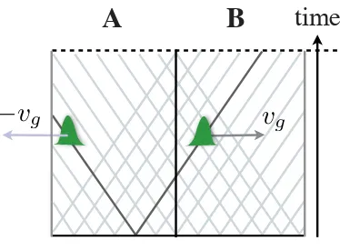
Below, in section V B, we will discuss how undergoing spontaneous emissions, i.e., incoherently scat-tering light from the lattice lasers or another source, tends to localise particles in the system, providing the environment with information about the location of the particles. In the typical limit for optical lattice experiments, this localisation essentially projects a particle onto a single lattice site (although we typically cannot or do not measure which site this was). This localisation in space delocalises the atom in quasi-momentum space across the first Brillouin zone, leading to a broadening of the quasi-momentum distribution and an increase in the kinetic energy beginning from the ground state. For hard-core bosons in 1D, these processes can be approximately described by the master equation

d

dtρ=−i[Hbos, ρ]− Γ 2

X

l

a†_lala†_lalρ+ρa†_lala†_lal−2a†_lalρa†_lal

, (49)

where Γ is the effective rate of spontaneous emission events.

As in the case of the optical Bloch equations, it is straight-forward to formulate the quantum trajectories approach for this master equation. Now we have a set of jump operators, with as many jump operators as we have lattice sites in the system andcm≡a†mam, i.e., the on-site number operator, and a corresponding

effective Hamiltonian

Heff =Hbos−i

Γ 2

X

m

a†mama†mam. (50)

Intuitively, this form for the jump operators makes sense, as application of a number operator on a given site, a†_lal|ψi/ka†lal|ψik, leads to the localisation of a single particle on site l. The probability that this

occurs on a particular sitelis proportional to the expectation value_h(a†_lal)2i, which reflects the fact that

0 2 4 6 8 10

−7

−6

−5

−4

−3

−2

−1 0

tJ EK

0 2 4 6 8 10

−7 −6 −5 −4 −3 −2

tJ

!

EK

"

1000 trajectories Exact

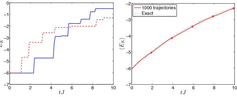
FIG. 5: Illustrative example of quantum trajectories averaging for a gas of hard-core bosons on a lattice, analogous to the example for a two-level system in Fig. 3. Here we show results from exact diagonalisation calculations with 5 particles on 10 lattice sites. (left) Kinetic energy of the system of hard-core bosons as a function of timetJfor two example trajectories (with blue solid and red dashed lines showing different random samples). We see the effect of quantum jumps, where the kinetic energy increases as individual atoms are localised in space, and hence spread over the Brillouin zone in quasi-momentum. Here the scattering rate Γ = 0.1J. (right) Values for the kinetic energy averaged over 1000 sample trajectories, compared with the exact result from eq. (51). As in the case of the two-level system, the quantum trajectories results agree with the exact results within the statistical errors, which are shown here as error bars calculated as described in section III C.

enhanced by superradiance [213, 214]. We will see below that this enhancement is related to the excitation of a collection of atoms in one site being symmetric.

The localisation of an atom on a single site corresponds to a spreading of the localised particle over all of the possible states in quasimomentum space, and hence to an increase in kinetic energy. This can be seen in Fig. 5, where we propagate states in time numerically using quantum trajectories. As for the previous case of the optical Bloch equations, we show two example trajectories as well as a trajectory average, here for the kinetic energy in the system as a function of time. By direct computation of expectation values from the master equation, we see that

d dtEbos≡

d

dthHbosi=−ΓhHbosi, (51) so thatEbos(t) =Ebos(t= 0) exp(−Γt). In the right hand panel of Fig. 5 we compare this analytical result

to the numerical value as a function of time, and observe very good agreement to within the estimated statistical error.

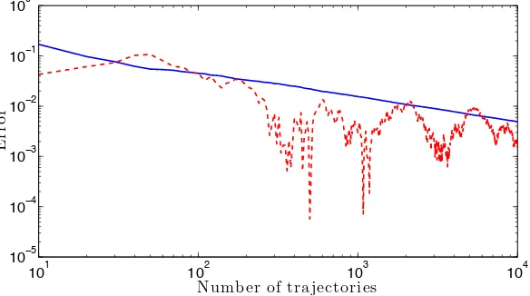
We investigate this statistical error as a function of the number of trajectories in Fig. 6. We fix the time at tJ = 8, and plot the statistical error and the discrepancy between the value of Ebos calculated

from the trajectory average and the exact value obtained from the master equation as a function ofNtraj.

The solid blue line represents the statistical error, and the dashed red line the discrepancy between the trajectory average and the exactly computed value. From the double logarithmic scale we see the scaling ∝1/√N. As in the example of the optical Bloch equations, we expect the means over different samples of trajectories to be approximately normally distributed, and therefore 68.2% of all possible samples should have discrepancies to exact values that fall below the estimated statistical error. The values shown here are again consistent with that analysis. In addition to this data, we also show using lighter (green) solid and dashed lines the same analysis for a local correlation function_h(a†5a6+a†6a5)i. We see that the relative

error is higher than for the globally averaged value, but the behaviour of the local correlation function with the number of trajectories is very similar.

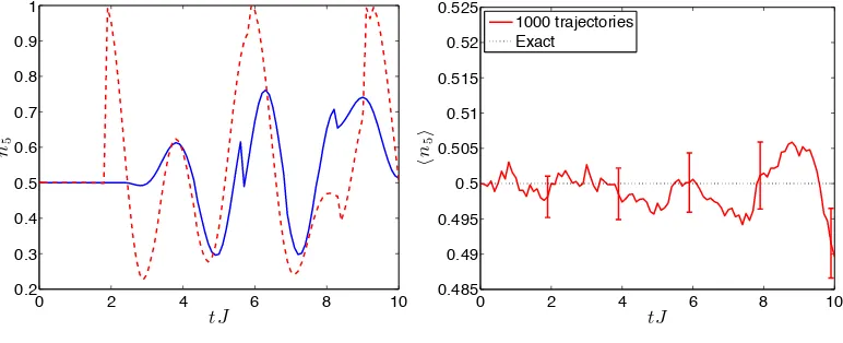
In Fig. 7 we show additional data for another local correlation function, namely the on-site density. This is quite instructive, because it shows how individual trajectories need not exactly enforce symmetries that are present in the master equation as a whole. Specifically, for a system with periodic boundary conditions and an initial density that is uniform across the system, we expect that

d dtha

†