Discovering bipartite substructure in directed networks

Discovering Bipartite Substructure in Directed

Networks

Alan Taylor

J. Keith Vass

Desmond J. Higham

August 13, 2010

Abstract

Bipartivity is an important network concept that can be applied to nodes, edges and communities. Here we focus on directed networks and look for subnetworks made up of two distinct groups of nodes, connected by “one-way” links. We show that a spectral approach can be used to find hidden substructure of this form. Theoretical support is given for the idealised case where there is limited overlap between subnetworks. Numer-ical experiments show that the approach is robust to spurious and missing edges. A key application of this work is in the analysis of high-throughput gene expression data, and we give an example where a biologically mean-ingful directed bipartite subnetwork is found from a cancer microarray data set.

1

Motivation

A bipartite network, or subnetwork, involves objects that may be split into two disjoint groups with connections only occurring across, but not within, the two groups. Sometimes this bipartivity is obvious because the objects naturally fall into two groups. For example, a Hollywood movie network could be constructed with nodes that are either actors or movies, with an edge denoting that an actor appeared in a movie. However, in other cases, bipartite structure might not be immediately apparent, and although there has been interest in deriving measures of the overall level of bipartivity in a network, node or edge [3, 6, 9], our focus

∗_{Department of Mathematics and Statistics, University of Strathclyde, Glasgow, G1 1XH,}

Scotland, [email protected].

†_{Translational Medical Research Collaboration, The Sir James Black Centre, University of}

Dundee, DD1 5EH, Scotland, [email protected]

‡_{Department of Mathematics and Statistics, University of Strathclyde, Glasgow, G1 1XH,}

here is on the practical issue of identifying hidden bipartite substructures. More precisely, we are concerned with discovering approximately bipartite subnetworks, because data sets are typically contaminated with missing and spurious edges.

Efforts in this direction have been applied to protein-protein interaction (PPI) networks, which have nodes given by proteins and edges denoting that two pro-teins have been observed to interact physically [2]. It is known that at least some types of protein-protein interaction arise through complementary binding domains, and in this case all proteins that possess one binding domain should interact with all proteins that share the complementary domain [14]. In [11], an algorithm was developed that aims to find bipartite substructure in PPI networks, thereby offering a route towards the identification of new binding domains using only interaction data. That algorithm uses spectral information—eigenvectors and eigenvalues of the adjacency matrix—and was shown to be robust in the presence of noise. The related approach in [5] compares the propensity for even and odd walk lengths between pairs of nodes by forming the negative matrix exponential. This allows the possibility of breaking down the whole network into quasi-bi-partite communities.

This work differs from previous studies by considering networks withdirected

edges—a connection from nodei to nodej does not necessarily have a matching

connection fromj toi. Our aim is to develop an approach for discoveringdirected

bipartite substructure, that is, groups of nodes S1 and S2, such that edges point

from nodes in S1 to nodes in S2. We will show that spectral information is

still relevant if we generalize from eigenvectors and eigenvalues to singular values and singular vectors. In section 2 we develop our theoretical arguments and in section 3 we test them on synthetically constructed networks, and compute some basic statistical measures. Finally, in section 4, we look at a larger network arising from cancer microarray data, and show that it is possible to discover biologically relevant directed bipartite subnetworks.

2

Relevance of the Singular Value

Decomposi-tion

Given a directed network with N nodes, we let the unsymmetric matrix A _∈

RN×N

denote the corresponding adjacency matrix, so thataij = 1 if there is a link

fromitoj andaij = 0 otherwise. To characterize directed bipartite subnetworks,

we find it useful to borrow thelock and key analogy that was introduced in [11].

We suppose that locks and keys are distributed among the nodes in a network. Each lock and key has a particular colour (red, blue, green, . . . ) and lock-key matches, corresponding to edges in the network, take place only when the colours

agree. Suppose two sets of nodes, S1 and S2, form a bipartite subnetwork; so

imagine thatS1 consists of all the nodes that possess a certain colour of key, say

red, and that S2 consists of all the nodes that possess the matching red lock.

We note that the reference [11] dealt only with undirected edges, whereas this work considers the directed case. So the concept of locks and keys here is slightly different, and perhaps more natural, and we find that the arguments supporting a spectral algorithm are stronger.

Focussing on this particular red lock-key subnetwork, we may introduce indi-cator vectors ured,vred_∈RN _{such that}

(ured)i =

1 if node ihas the red key,

0 otherwise, (1)

and

(vred)i =

1 if nodei has the red lock,

0 otherwise. (2)

It follows immediately that the edges arising from red key-lock interactions may

be characterized through the outer product ured(vred)T_{. If we let keyred :=}

||ured_||2₂ and lockred := _||vred_||2₂ denote the total number of red keys and red locks, respectively, then this outer product may be written

p

keyred_×lockred ubred(bvred)T_,

where ubred := ured/_||ured_||2 and vbred := vred/||vred||2 are unit vectors. More

generally, when all link arise through key-lock interactions, the adjacency matrix for the network may be expanded as

A = signpkeyred_×lockred bured(bvred)T +pkeyblue_×lockblueubblue(vbblue)T

+pkeygreen_×lockgreen ubgreen(vbgreen)T _{+. . ., (3)}

where the sign function deals with the possibility of multiple key-lock matches;

nodeimay have both a red and blue key whilst node j has both a red and a blue

lock.

The sign function in (3) is not needed if make the following assumption.

Assumption A: each node has at most one key and one lock.

Note that this assumption permits a node to possess a key of one colour and a lock of another colour, or a lock and key of the same colour. A second important con-sequence of Assumption A is that the key indicator vectors_{ured,ublue,ugreen, ..._}

form an orthogonal set and the lock indicator vectors_{vred,vblue,vgreen, ..._} form an orthogonal set. In this case, we see that the expansion (3) has the same form as the singular value decomposition (SVD) [7]

A=

N

X

k=1

where σ1 ≥ σ2 ≥ · · ·σN ≥ 0 are the singular values of A, and {u[k]}Nk=1 and

{v[k]_}N

k=1 are the corresponding left and right singular vectors, respectively. We

conclude that under Assumption A the SVD can be used to discover bipartite

subgraphs—the square of the singular value, σ2

k, indicates the product of the

number of locks and keys of the kth colour, the nonzero entries of u[k] _{give the}

key locations and the nonzero entries ofv[k] _{give the lock locations.}

We show now that there is a complementary way to motivate the use of the SVD. This approach, which is based on the ideas in [11] that were used for undirected networks, also goes some way towards allowing for false negatives

among the edges. Under Assumption A, suppose that node i does not possess

the red key. Then multiplying the ith row of the adjacency matrix into the red

lock indicator vector will give a value zero; there will be no matches in the inner

product. On the other hand, if node i possesses the red key then multiplying

the ith row of the adjacency matrix into the red lock indicator vector will count

the number of red locks in existence—each red lock will take part in one nonzero term. Suppose now that there are some “errors” in the network in the form of

missing edges. More precisely, suppose that only a fixed proportionθ _∈(0,1) of

the red key-lock matches are recorded as edges. Then generalizing the argument above we have

Av[k] i =

N

X

j=1

aijv[ k]

j =

θlockred if node i has the red key,

0 otherwise,

which may be written

Avbred =θplockred_×keyredubred. (5)

Similarly, we find that

AT

b

ured =θplockred_×keyredvbred. (6)

The relations (5) and (6) show that bured and vbred correspond to left and right

singular vectors of A, respectively, with singular value θ√lockred_×keyred. Of

course, when θ = 1, we recover the singular value expression √lockred_×keyred

that we derived earlier via the argument involving rank one outer products. How-ever, it is worth noting that (5) and (6) require Assumption A to hold only for nodes with red keys or locks. The other nodes in the network could be con-nected in any way. So the SVD will reveal isolated substructure hidden within any complex network.

Figure 1: Example with 3 lock-and-key types.

network, where the nodes will typically be labelled in a manner that hides the bipartivity, the singular values σ1, σ2, . . . can be taken in order, and the indices

of extremal components in the corresponding left and right singular vectors used to identify candidate nodes.

Eigenvectors and, more generally, singular vectors, enjoy important varia-tional properties, and hence the information that they convey tends to be robust to the presence of noise. This has been confirmed experimentally; see, for exam-ple, [1, 4, 8, 10, 12, 17]. In particular, for the case of undirected edges, it was shown in [11] that the SVD can find approximate bipartite subgraphs in both synthetic and real networks. In the next section, we test the robustness of the SVD in the directed network setting.

3

Exploratory Tests

3.1

Detailed Example

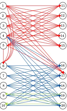
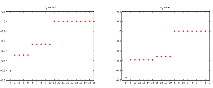
The directed network in Figure 1 does not completely satisfy Assumption A from section 2. The colour coding of the arrows in Figure 1 is designed to emphasize the lock and key distribution. Nodes 1–5 have the red key and nodes 6, 11–15 and 17 the corresponding red lock. Nodes 4 and 6–10 have the blue key and nodes 16–20 the corresponding blue lock. Finally, nodes 19 and 20 have the green key, while nodes 9 and 10 have the green lock. We note that this node ordering was chosen simply to make the output easier to interpret—results from the SVD are invariant under symmetric row and column permutations.

4 1 2 3 5 6 7 8 9 10 13 20 11 19 12 18 17 14 15 16 −0.6

−0.5 −0.4 −0.3 −0.2 −0.1 0 0.1

u₁ sorted

17 6 11 12 13 14 15 16 18 19 20 5 8 10 1 4 9 7 3 2 −0.5

−0.4 −0.3 −0.2 −0.1 0 0.1 0.2

v₁ sorted

Figure 2: First left and right singular vectors for network in Figure 1.

consistent with our expectation that the first, second and third pairs of singular vectors should correspond to the red, blue and green groups.

3.1.1 First left and right singular vectors

Figure 2 shows the components of the first left and right singular vectors of the adjacency matrix in increasing order. On the horizontal axis are the indices, so, for example, the most negative left and right singular vector entries correspond to nodes 4 and 17, respectively.

For the first left singular vector, u[1], there are two main groups of nodes

with components away from zero; one with values around ₋0.34 and another

with values around₋0.23. There is also an outlying vertex at around₋0.5. The group at height ₋0.34 involves nodes 1,2,3,5, which, as we see from Figure 1, share the red key. The outlier is node 4. This is the only other red key node, but it also has the blue key.

The first right singular vector, v[1], splits up the network in a similar fashion. Nodes 6, 11, 12, 13, 14 form a clear group and we see from Figure 1 that they share the red lock. The outlier is node 17. This is the only other red lock node, but it also has the blue lock. We note that node 6 differs from its neighbours in Figure 2 in that it also has a blue key, but the left singular vector has not been affected by this—node 6 is placed at the same height as the purely red lock nodes. This consistent with the theory in section 2, where Assumption A does not rule out the case of a node having a key and lock of different colours.

In Figure 3 we show the adjacency matrix for the subgraph created by nodes 4, 1, 2, 3, 5, 6, taken from the left hand end of u[1] up to the cut-off from ₋0.34 to₋0.23, and nodes 17, 6, 11, 12, 13, 14, 15, taken from the left hand end ofv[1]

1 2 3 4 5 6 11 12 13 14 15 17 1

2 3 4 5 6 11 12 13 14 15 17

nz = 36 Submatrix

Figure 3: Subgraph showing red lock-key interactions arising from nodes

4,1,2,3,5 and 17,6,11,12,13,14,15 taken fromu[1] _{and v}[1] _{in Figure 2.}

Similarly, Figure 4 reveals the blue lock-key interactions by plotting the adja-cency matrix arising from nodes 6,7,8,9,10 and 16,18,19,20 that were grouped together above the main cut-offs in Figure 2. Here, node 17 is missing from the blue lock group; this makes sense because it is also a lock member of the larger

red lock-key group. In Figure 4 we also see that the green lock-key group of 9,10

and 19,20 appears as a block in the adjacency matrix. However, from Figure 2

this appears to be a coincidental feature caused by the fact that these node are

also part of the blue subgraph—the components of nodes 9,10 in u[1] and 19,20

in v[1] are not visually distinguishable from their blue key and lock neighbours,

6,7,8 and 16,18, respectively.

Overall, the first left and right singular vectors have done an excellent job of sorting out the key and lock nodes, respectively, for the red group. They also made a reasonable delineation of the blue group, but the ambiguous nodes that shared red and blue characteristics were placed next to their red colleagues, which form the dominant group.

3.1.2 Second left and right singular vectors

Figure 5 shows the second left and right singular vectors. In u[2] we see that

nodes 1,2,3,5 are grouped together. These are four out of the five red key nodes. Node 4, which also has the blue key, has been given a positive value, in line with the positivity of nodes 6, 7, 8, 9, 10, which complete the blue key group and are

classified together. In v[2] we see nodes 6, 11, 12, 13, 14, 15 grouped together.

6 7 8 9 10 16 18 19 20 6

7

8

9

10

16

18

19

20

nz = 24 Submatrix

Figure 4: Subgraph showing blue lock-key interactions arising from nodes 6,7,8,9,10 and 16,18,19,20 taken from u[1] _{and v}[1] _{in Figure 2.}

classified together.

So, overall, the second singular vectors also give information about both red and blue groups, but they favor the second-largest, blue group.

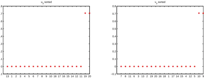
3.1.3 Third left and right singular vectors

Figure 6 shows the third left and right singular vectors. In this case we see that the

green keys, 19,20 and the green locks 9,10 have been picked out unambiguously.

1 3 2 5 15 14 13 18 12 20 11 19 17 16 4 6 7 8 9 10 −0.4

−0.3 −0.2 −0.1 0 0.1 0.2 0.3 0.4

u₂ sorted

6 11 12 13 14 15 3 8 7 9 1 4 10 5 2 17 16 18 19 20 −0.3

−0.2 −0.1 0 0.1 0.2 0.3 0.4

v₂ sorted

13 1 2 3 4 5 6 7 8 9 10 18 17 16 15 14 12 11 19 20 −0.1

0 0.1 0.2 0.3 0.4 0.5 0.6 0.7 0.8

u₃ sorted

7 8 11 6 3 13 2 19 20 16 18 1 17 14 15 4 12 5 10 9 −0.1

0 0.1 0.2 0.3 0.4 0.5 0.6 0.7 0.8

v₃ sorted

Figure 6: Third left and right singular vectors for network in Figure 1.

3.2

Parameterized Example

Our second experiment tests the robustness of the SVD approach when spurious and missing edges contaminate the directed bi-partivity. We constructed a

net-work of 50 nodes with nodes 1–10 forming group S1 and nodes 11–25 forming

groupS2. We formed links independently at random such that the probability of

a link from nodeito nodej is given by 0.6 ifi_∈S1 andj ∈S2, andp2 otherwise.

To the left in Figure 7 we show the adjacency matrix that arose forp2 = 0.1.

We see that the S1-to-S2 block forms a dense patch, but there is a significant

amount of non-bipartite ‘noise’. In fact there are 94 S1-to-S2 edges and 226

others. In the centre and left of Figure 7 we show the first left and right singular vectors. It is clear that the key group,S1, is picked out byu[1]and the lock group,

S2, is picked out by v[1]; in each case the group members appear sequentially,

taking the extreme values in the vector.

In Figure 8, we increase p2 to 0.3. Now there are 665 edges outside the S1

-to-S2 class. In this case we are at the extremes of the noise level that the SVD can

tolerate. Inu[1], the 10 nodes in groupS1 appear in positions 1, 2, 3, 4, 6, 7, 10,

11, 13, 20 as we search through the components with largest to smallest absolute value. Similarly, inv[1], the 15 nodes in group S2 appear in positions 1, 2, 3, 4,

5, 8, 9, 10, 11, 14, 15, 16, 20, 29, 31. So the dominant singular vectors do not reproduce perfectly the key and lock groups; although at this high level of noise it may be argued that the groups are not clearly defined.

3.3

Statistical Testing

Having established that the left and right singular vectors may be useful in iden-tifying members of directed bipartite communities, we would like to assess the success with which nodes are classified into subgroups. To this end we construct

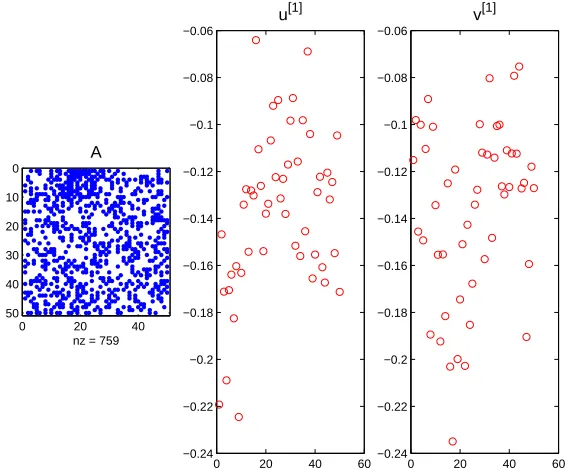
0 20 40 0 10 20 30 40 50

nz = 320

A

0 20 40 60 −0.45 −0.4 −0.35 −0.3 −0.25 −0.2 −0.15 −0.1 −0.05 0 u[1]

0 20 40 60 −0.35 −0.3 −0.25 −0.2 −0.15 −0.1 −0.05 0 0.05 v[1]

Figure 7: Left: adjacency matrix. Middle: first left singular vector. Right: first right singular vector. Herep2 = 0.1 for the non-bipartite connectivity probability.

0 20 40 0 10 20 30 40 50

nz = 759

A

0 20 40 60 −0.24 −0.22 −0.2 −0.18 −0.16 −0.14 −0.12 −0.1 −0.08 −0.06 u[1]

0 20 40 60 −0.24 −0.22 −0.2 −0.18 −0.16 −0.14 −0.12 −0.1 −0.08 −0.06 v[1]

1–10 and 11–20, respectively. We connect pairs of nodes i and j independently

at random with probability p1 if i ∈ S1 and j ∈ S2 and with probability p2

otherwise.

With an adjacency matrix set up in this fashion, we may compute the SVD and examine the components of the first left and right singular vectors. If the SVD perfectly organises nodes into the appropriate subgroups, then nodes

1-10 should correspond to the ten components with highest absolute value in u1

and nodes 11-20 should correspond to the ten components with highest absolute value in v1. We fix p1 and vary p2 from 0 to p1, generating several instances of

the synthetic network described above for each value of p2. The SVD of each

adjacency matrix is calculated and the proportion of correctly identified nodes in the first ten positions of the relevant singular vector is recorded in each instance. In Figure 9 we show a plot of the mean proportion of correctly identified nodes

for p1 = 0.9 and p2 varying from 0 to 0.9 in increments of 0.01. The blue line

shows the mean proportion of “key” nodes correctly identified and the red line corresponds to the mean proportion of “lock” nodes correctly identified. In this case the probability of false negatives in the region of bipartite connectivity is 0.1, and the SVD is reasonably tolerant of false positives elsewhere in the adjacency matrix. The singular vectors correctly identify more than half of the correct nodes until the probability of a false positive in a given position in the adjacency matrix reaches around 0.3.

Figure 10 shows a plot of the same type with p1 = 0.6. In this case, the

singular vectors successfully identify more than half of the corect nodes until the probability of a false positive in a given position in the adjacency matrix reaches around 0.15.

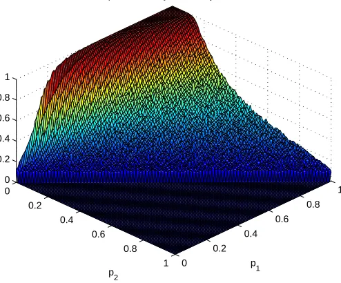
By varying p1 from 0 to 1 and carrying out the procedure described above,

we can obtain three dimensional plots of the proportions of locks and keys cor-rectly recovered by the SVD for varying probabilities of false negatives and false positives. Figure 11 shows the proportion of ‘key’ nodes correctly recovered for varying values ofp1 and p2. The data is also plotted as a heat map in Figure 12.

Similarly, Figures 13 and 14 show the proportion of ‘lock’ nodes correctly recov-ered as a surface plot and a heat map, respectively. By inspection we see that the left and right singular vectors perform very similarly in their identification of ‘lock’ and ‘key nodes’. Approximately half the correct nodes are identified if the probability of a false positive is around a third of the probability of a ‘true pos-itive’, and all the correct nodes are identified if every true connection is present and the probability of a false positive is less than 0.2.

0 0.1 0.2 0.3 0.4 0.5 0.6 0.7 0.8 0.9 0

0.1 0.2 0.3 0.4 0.5 0.6 0.7 0.8 0.9 1

Probability of false positives

Proportion of group members correctly identified

Figure 9: Proportion of ‘key’ nodes (red) and ‘lock’ nodes (blue) correctly iden-tified by first singular vectors forp1 = 0.9 with varying levels of ‘noise’.

0 0.1 0.2 0.3 0.4 0.5 0.6 0.7

0 0.1 0.2 0.3 0.4 0.5 0.6 0.7 0.8 0.9 1

Probability of false positives

Proportion of group members correctly identified

0 0.2

0.4 0.6

0.8

1 0

0.2 0.4

0.6 0.8

1 0

0.2 0.4 0.6 0.8 1

p

1

Proportion of ‘keys’ correctly identified

p

2

Figure 11: Proportion of ‘key’ nodes correctly identified by first left singular vector for varying levels of ‘noise’.

Having quantified the success of the SVD in a number of test cases, we now apply our method to a dataset from genomics and attempt to uncover meaningful communities.

4

Application to Cancer Microarray Data

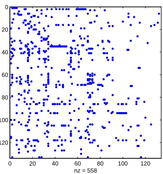
In this section we consider a network arising through gene expression. Cancer microarray data from [15] was treated with the classification method developed in [16]. More precisely, we selected 133 genes related to the oncogene p53, and

com-puted the ‘plus-minus’ network. Here, an edge between nodes i and j indicates

that when gene i expresses significantly above its usual level, gene j generally

expresses significantly below its usual level. This produced a directed network with 133 nodes and 558 edges, whose adjacency matrix is shown in Figure 15. Discovering directed bi-partite subgraphs in this setting is of major biological interest, as it reveals a pair of gene groups such that over-expression in one group is associated with under-expression in the other.

0.1 0.2 0.3 0.4 0.5 0.1

0.2 0.3 0.4 0.5 0.6 0.7 0.8 0.9 1.0

Proportion of ‘keys’ correctly recovered

0.1 0.2 0.3 0.4 0.5 0.6 0.7 0.8 0.9

Figure 12: Proportion of ‘key’ nodes correctly identified as a heat map.

0 0.2

0.4 0.6

0.8

1 0

0.2 0.4

0.6 0.8

1 0

0.2 0.4 0.6 0.8 1

p₁ Proportion of ‘locks’ correctly identified

p₂

0.1 0.2 0.3 0.4 0.5 0.1

0.2 0.3 0.4 0.5 0.6 0.7 0.8 0.9 1.0

Proportion of ‘locks’ correctly recovered

0.1 0.2 0.3 0.4 0.5 0.6 0.7 0.8 0.9

Figure 14: Proportion of ‘lock’ nodes correctly identified as a heat map.

0 20 40 60 80 100 120 0

20

40

60

80

100

120

nz = 558

0 20 40 60 80 100 120 140 0

1 2 3 4 5 6 7 8 9

i Σi

Figure 16: Singular values of the adjacency matrix from Figure 15.

0 20 40 60 80 100 120 140 −0.2

−0.1 0 0.1 0.2 0.3 0.4 0.5

u₂ sorted

0 20 40 60 80 100 120 140 −0.2

−0.15 −0.1 −0.05 0 0.05 0.1 0.15 0.2 0.25

v₂ sorted

Figure 17: Second left and right singular vectors of the adjacency matrix from Figure 15.

which are shown in Figure 17.

Keeping in mind the typical network size suggested by the singular values and considering the natural break-points in the singular vector components, we chose

the indices from four extreme components ofu[2] and seven extreme components

of v[2]. This produced the subnetwork shown in Figure 18. We see that there

is a high degree of directed bi-partivity. Denoting the first four nodes in this

subnetwork as groupS1 and the remaining seven nodes as group S2, twenty-five

out of the possible twenty-eightS1-to-S2 connections are present, but none of the

86 118 94 35 39 40 42 49 100 24 23 86

118 94 35 39 40 42 49 100 24 23

nz = 25 Submatrix

Figure 18: Adjacency matrix for the subgraph of 11 nodes discovered via the second singular vectors.

The subnetwork in Figure 18 was produced using only the network data. Because of the high level of interest in p53, there is extra biological information available, which can be used to justify the relevance of the subnetwork. Details of the genes are given in Table 1. Looking at these genes, BTG2, CCNG2 and FHL1 all appear to have inhibitory effects on growth or cell-division, while the role of HLA-F with respect to growth is unclear. KIF15, CDC20, PRC1, CCNB2, KIF20A and NEK2 all seem to be involved in the cell-division process and, in most cases, inhibiting the genes seems to prevent growth. So it appears that we have identified two groups of genes whose products have opposite functions; whilst we make no detailed biological interpretation here it seems reasonable that their mutually exclusive expression patterns are consistent with growth promotion and inhibition being correlated; with one of these groups being switched on when the other is off.

sub-Probe set ID Gene ID Description

201235_s_at _{BTG2 BTG family, member 2}

202769_at _{CCNG2 Cyclin G2}

201540_at _{FHL1 four and a half LIM domains 1}

221978_at _{HLA-F major histocompatibility complex, class I, F}

219306_at _{KIF15 kinesin family member 15}

202870_s_at _{CDC20 CDC20 cell division cycle 20 homolog (S. cerevisiae)}

218009_s_at _{PRC1 protein regulator of cytokinesis 1}

204822_at _{TTK TTK protein kinase}

202705_at _{CCNB2 cyclin B2}

218755_at _{KIF20A kinesin family member 20A}

204641_at _{NEK2 NIMA (never in mitosis gene a)-related kinase 2}

Table 1: Details of genes corresponding to the groups in Figure 18. The two groups are separated by a double horizontal line.

matrix. This indicates that the degree of bipartivity seen in Figure 18 is unlikely to have arisen “by chance.”

Overall, we believe that these initial results show a proof of principle for the SVD as a tool for discovering directed bipartite communities. In the context of analysing high-throughput expression data its main utility, of course, will lie in the case where directed bipartite patterns are found that involve gene groups for which annotational information is missing or only partially known. In this way, the algorithm could suggest putative functional and cause-and-effect rela-tionships that may direct more specific experiments. More generally, for any set of unsymmetric interaction data this new method for detecting directed bipartite community structure offers a useful tool for highlighting meaningful information.

References

[1] D. Barash,Second eigenvalue of the Laplacian matrix for predicting RNA

conformational switch by mutation, Bioinformatics, 20 (2004), pp. 1861– 1869.

[2] E. de Silva and M. P. H. Stumpf,Complex networks and simple models

in biology, J. R. Soc. Interface, 2 (2005), pp. 419–430.

[3] E. Estrada,Protein bipartivity and essentiality in the yeast protein-protein

interaction network, J. Proteome Res., 5 (2006), pp. 2177–2184.

[4] E. Estrada and N. Hatano, Communicability in complex networks,

[5] E. Estrada, D. J. Higham, and N. Hatano,Communicability and mul-tipartite structures in complex networks at negative absolute temperatures, Physical Review E, 78 (2008), p. 026102.

[6] E. Estrada and J. Rodr´ıguez-Vel´azquez, Spectral measures of

bi-partivity in complex networks, Physical Review E, 72 (2005), p. 046105.

[7] G. H. Golub and C. F. Van Loan,Matrix Computations, Johns Hopkins

University Press, Baltimore, third ed., 1996.

[8] P. Grindrod and M. Kibble,Review of uses of network and graph theory

concepts within proteomics, Expert Review of Proteomics, 1 (2004), pp. 229– 238.

[9] P. Holme, F. Liljeros, C. R. Edling, and B. J. Kim, Network

bi-partivity, Physical Review E, 68 (2003), p. 056107.

[10] Y. Hu and J. A. Scott, HSL_MC73: A fast multilevel Fiedler and

pro-file reduction code, RAL-TR-2003-36, Numerical Analysis Group, Computa-tional Science and Engineering Department, Rutherford Appleton Labora-tory, 2003.

[11] J. L. Morrison, R. Breitling, D. J. Higham, and D. R. Gilbert,A

lock-and-key model for protein-protein interactions, Bioinformatics, 2 (2006), pp. 2012–2019.

[12] A. Spence, Z. Stoyanov, and J. K. Vass, The sensitivity of spectral

clustering applied to gene expression data, in Proceedings of the 1st Inter-national Conference on Bioinformatics and Biomedical Engineering, 2007, pp. 1343–1346.

[13] A. J. Taylor, Computational Tools for Complex Networks, PhD thesis,

University of Strathclyde, 2009.

[14] A. Thomas, R. Cannings, N. A. M. Monk, and C. Cannings,On the

structure of protein-protein interaction networks, Biochemical Soc. Tranl., 31 (2003), pp. 1491–1496.

[15] P. J. Valk, R. G. Verhaak, M. A. Beijen, C. A. Erpelinck, S. B.

van Waalwijk van Doorn-Khosrovani, J. M. Boer, H. B.

Bever-loo, M. J. Moorhouse, P. J. van der Spek, B. L¨uwenberg, and

R. Delwel, Prognostically useful gene-expression profiles in acute myeloid

leukemia, New England J. Medicine, 16 (2004), pp. 1617–1628.

[16] J. K. Vass, D. J. Higham, X. Mao, and D. Crowther,New controls of

Tech. Rep. Department of Mathematics 10 (2009), University of Strathclyde, Glasgow, UK, 2009.

[17] C. Walshaw and M. Cross, JOSTLE: Parallel multilevel