A parametric study on creep-fatigue strength of welded joints using the linear matching
method
Yevgen Gorash, Haofeng Chen∗
Department of Mechanical&Aerospace Engineering, University of Strathclyde, James Weir Building, 75 Montrose Street, Glasgow G1 1XJ, UK
Abstract
This paper presents a parametric study on creep-fatigue strength of the steel AISI type 316N(L) weldments of types 1 and 2 according to R5 Vol. 2/3 Procedure classification at 550◦C. The study is implemented using the Linear Matching Method (LMM)
and is based upon a latest developed creep-fatigue evaluation procedure considering time fraction rule for creep-damage assessment. Parametric models of geometry and FE-meshes for both types of weldments are developed in this way, which allows variation of parameters governing shape of the weld profile and loading conditions. Five configurations, characterised by individual sets of parameters, and presenting different fabrication cases, are proposed. For each configuration, the total number of cycles to failure
N? in creep-fatigue conditions is assessed numerically for different loading cases including normalised bending moment ˜M and
dwell period∆t. The obtained set of N? is extrapolated by the analytic function, which is dependent on ˜M,∆t and geometrical
parameters (αandβ). Proposed function for N?shows good agreement with numerical results obtained by the LMM. Thus, it is
used for the identification of Fatigue Strength Reduction Factors (FSRFs) intended for design purposes and dependent on∆t,α,β.
Keywords: Creep, Damage, Finite element analysis, FSRF, Low-cycle fatigue, Type 316 steel, Weldment
1. Introduction
According to industrial experience, during the service life of welded structures subjected to cyclic loading at high tem-perature, welded joints are usually considered as the critical locations of potential creep-fatigue failure. This is caused by higher stress concentration, altered and non-uniform material properties of weldments compared to the parent material of the entire structure. Therefore, creep and fatigue characteris-tics of welded joints are of a priority importance for long-term integrity assessments and design of welded structures. There were attempts to develop analytical tools [1] to estimate long-term strength of welded joints under variable loading. How-ever, residual life assessments are frequently complicated and inaccurate because of complex material microstructure and too many parameters affecting the strength of welded joints. They include technological parameters of welding process and post-weld heat treatment, accuracy of modelling of post-weldment ma-terial microstructure, influence of residual stresses and distor-tions, geometrical parameters of the shape of the weld pro-file and non-welded root gaps, parameters of service conditions such as temperature, mechanical loading and dwell period. In view of the complexity of a unified model development for the assessment of creep-fatigue strength, there are a limited number of existing analytical approaches, but none of which are able to account for all of weldment parameters mentioned above. Thus,
∗Corresponding author. Tel.:+44 141 5482036; Fax:+44 141 5525105.
Email address:[email protected](Haofeng Chen)
URL:http://www.thelmm.co.uk(Haofeng Chen)
long-term strength of weldments is a wide research area, which requires some unified integral approach able to improve the life prediction capability for welded joints. The most comprehen-sive overviews of studies devoted to investigation of influence of various parameters on fatigue life of welded joints are pre-sented in [1, 2, 3]. However, the influence of creep on residual life is not investigated in these works.
This paper presents further extension of a latest developed approach [4], which includes a creep-fatigue evaluation proce-dure considering time fraction rule for creep-damage assess-ment and a recent revision of the Linear Matching Method (LMM) to perform a cyclic creep assessment [5]. The appli-cability of this approach to a creep-fatigue analysis was veri-fied in [4] by the comparison of FEA/LMM predictions for an AISI type 316N(L) steel cruciform weldment at 550◦C with
ex-periments by Bretherton et al. [6, 7, 8, 9] with the overall ob-jective of identifying fatigue strength reduction factors (FSRF) of austenitic weldments for further design applications. An overview of previous modelling studies devoted to analysis and simulation of these experiments [6, 7, 8, 9] is given in [4]. Gen-erally they investigated an accuracy of residual life assessments according to R5 creep-fatigue crack initiation procedure [10] and its more recent revisions and potential improvements.
Di-rect Cyclic Analysis [11, 12] and the LMM framework [13, 14]. The LMM is distinguished from the other simplified methods by ensuring that both the equilibrium and compatibility are sat-isfied at each stage [13, 14, 15, 16]. In addition to the shake-down analysis method [15], the LMM has been extended be-yond the range of most other direct methods by including the evaluation of the ratchet limit [13, 14, 16] and steady-state cyclic behaviour with creep-fatigue interaction [17, 18]. The LMM ABAQUS user subroutines [19] have been consolidated by the R5 Procedure [10] research programme of EDF Energy to the commercial standard, and are counted to be the method most amenable to practical engineering applications involving complicated thermo-mechanical load history [14, 16]. Follow-ing this, the LMM was much improved both theoretically and numerically [5] to include more accurate predictions of the sta-bilised cyclic response of a structure under creep-fatigue condi-tions. This, in turn, allowed more accurate assessments of the resulting cyclic and residual stresses, creep strain, plastic strain range, ratchet strain and elastic follow-up factor. Finally, to aid wider adoption of the LMM as an analysis tool for industry, the development of an Abaqus/CAE plug-in with GUI has been started [20]. For this purpose, the UMAT subroutine code has been significantly updated [20] to allow use of multi-processors for the FE-calculations of shakedown and ratchet limits.
The parametric study presented in this paper is based on the research outcomes given in prior work [4] validated by match-ing the basic experiments [6, 7, 8, 9]. These outcomes briefly include: 1) more realistic modelling of a material behaviour of the weld regions (including LCF and creep endurance) when compared to previous studies; 2) a creep-fatigue evaluation pro-cedure considering time fraction rule for creep-damage assess-ment and a non-linear creep-fatigue interaction diagram; 3) ap-plication of the recent revision of the LMM outlined in [5]. As a result, the approach proposed in [4] provides the most accu-rate numerical prediction of the experiments [6, 7, 8, 9] with less conservatism when compared to previous works, particu-larly to [18]. Thus, exactly the same assessment approach is used in the current study and is applied to parametric studies of the weldment geometry in order to assess the effect on the predicted life.
Another outcome of the previous work [4] is the formulation of an analytical function for the total number of cycles to fail-ure N?in creep-fatigue conditions, which is dependent on
nor-malised bending moment ˜M and dwell period∆t. This function N?( ˜M,∆t) matches the LMM predictions with reasonable
ac-curacy and is used for the investigation of∆t influence on the
FSRF. Therefore, the effect of creep on long-term strength of type 2 dressed weldments (according to the classification in R5 Vol. 2/3 Procedure [10]) is taken in to account.
Apart from accounting for operational parameters ( ˜M and
∆t), it is necessary to investigate the influence of a weld profile
geometry on creep-fatigue strength within a parametric study. The introduction of geometrical parameters into the function
N?( ˜M,∆t) allows the calculation of the FSRF as a continuous
function able to cover a variety of weld profile geometries in-cluding type 1 and 2 in dressed, as-welded and intermediate configurations.
R2
thk 60°
h2
haz
α
D
β
α
thk
40°
haz
α
α
M
M
M
type 2
type 1
R1
δ
d2
h2
h1
d1 thk
[image:2.612.293.542.24.335.2]2
Figure 1: Designations of parameters fully describing weld profile geometries of types 1 and 2 weldments and applied bending moment, according to [6]
2. Parametric models of weldments
Referring to [1], generally creep-fatigue test results of weld-ment specimens contain various levels of scatter, which is usu-ally caused by geometric and processing variations such as part fit-up, weld gap, variation in feed rates, travel rates, weld an-gles, etc. This scatter complicates the interpretation of test re-sults, and often makes it nearly impossible to differentiate the effects of geometry, material non-uniformity, residual stress and other factors. It has been indicated [1] that one of the most crit-ical factors affecting the creep-fatigue life of a welded joint is the consistency of the cross-sectional weld geometry. The sim-plified weld profile is usually characterised by the following geometric parameters [1]: plate thickness, effective weld throat thickness, weld leg length, weld throat angle, and weld toe ra-dius. In this case the weld profile is assumed to be circular for type 1 and triangular for type 2 weldments with fillets on toes connecting with parent plates. A vast quantity of research re-viewed in [1, 2, 3] has been devoted to investigation of effects produced by these parameters on residual life.
weld-ment specimen contains 2 symmetric double-sided T-butt cruci-form fillet welds. The parent material for the manufacturing of all specimens are continuous plates of width w=200 mm and thickness thk =26 mm made of the steel type AISI 316N(L). The typical division of the weld into three regions is adopted here analogically to [4] including: parent material, weld metal and heat-affected zone (HAZ). It should be noted that the HAZ thickness is assumed to be 3mm based on the geometry given in [6]. These 3 regions have different mechanical properties de-scribed by the following material behaviour models and corre-sponding constants at 550◦C in [4] for the FEA with the LMM: • Elastic-perfectly-plastic (EPP) model for the design limits
as a result of shakedown analysis;
• Ramberg-Osgood (R-O) model for the plastic and total strains under saturated cyclic conditions;
• S–N diagrams for the number of cycles to failure caused by pure low-cycle fatigue (LCF);
• Power-law model in “time hardening” form for creep strains during primary creep stage;
• Reverse power-law relation for the time to creep rupture caused by creep relaxation during dwells;
• Non-linear diagrams for creep-fatigue damage interaction for the estimation of total damage.
The profile geometry of type 2 weldment is comprehensively characterised by one of two pairs of parameters: (1) indepen-dent parameters (αandβ), which are not dependent on a plate thickness thk, and (2) technologically controlled parameters (R2 and D), which change their values with a change of plate thick-ness thk. The advantage of the 1st couple is that it is not sensi-tive to simple scale transformation of the weldment geometry. The advantage of the 2nd couple is that it could be easily mea-sured and controlled according to technological requirements. Therefore, in parametric relations for strength of type 2 weld-ments the independent parameters (α and β) should be used with a capability of transformation into controlled parameters (R2and D). As illustrated in Fig. 1, angleαrepresents a local geometrical non-uniformity caused by a deviation from the tan-gent condition between parent plate and weld. Angleβ repre-sents a global geometrical non-uniformity caused by deposition of weld metal connecting the orthogonal part.
The relations between the two parameter pairs (α,βand R2, D) for a type 2 weldment are formulated using basic
trigono-metric calculus in conjunction with the thickness of a plate cross-section thk and the corresponding associated parameters (h2and d2) as illustrated in Fig. 1:
h2= thk
8.6666 and d2=
thk
2 +h2+
thk−h2
2 tan 60
◦. (1)
The direct transitions are formulated as follows
R2=
thk/2 cos (α+β)−
d2 sin (α+β) sinα
sin (α+β)−
cosα cos (α+β)
and
D=2R2 cosα+thk/2 cos (α+β) −2 R2.
(2)
The reverse transitions are formulated as follows
β=arccos
d2
2+(thk/2) 2
−R2
2−(R2+D/2) 2
−2 R2(R2+D/2)
,
α=90◦−arctan thk
2 d2 !
−β
−arccos
R2
2−(R2+D/2) 2
−d2
2−(thk/2) 2
−2 (R2+D/2) q
d2
2−(thk/2) 2
.
(3)
Relations between independent parameterαand controlled parameter δfor type 1 weldment are formulated using basic trigonometric calculus in conjunction with the thickness of a plate cross-section thk and the corresponding associated param-eters (h1and d1) as illustrated in Fig. 1:
h1= thk
13 and d1 =
thk−h1
2 tan 40
◦. (4)
The direct transition is formulated as follows
δ=R1(1−cosα) with R1=d1/sinα. (5) The reverse transition is formulated as follows
α=arccos R1−δ
R1 !
with R1= δ 2 +
d2 1
2δ. (6)
Since the proposed parameters for both types of weld profile are fully convertible, they can be used to characterise different scales of technological dressing of weldments by grinding such as dressed, as-welded and intermediate. Thus, in order to re-duce the computational costs, only five configurations of weld profile, listed in Table 1, were chosen for parametric study from among the possible parameter combinations. It should be noted that configuration no. 2 of the type 2 weldment titled “typically dressed” (characterised in Fig. 1 by h2 =3 mm, R2 =25 mm, D=59 mm,α=7.745◦andβ=38.382◦) has been an object of
research in prior work [4]. Configuration no. 1 is characterised by a tangent condition between parent plate and weld profile contours. Configuration no. 5 presents the extreme variant of a roughly manufactured welded joint without any dressing. Thus, configurations no. 2, 3 and 4 correspond to some intermediate variants of weldment fabrication between the scales “perfectly dressed” and “coarsely as-welded”.
Table 1: Geometrical configurations of weld profiles for type 1 and 2 weldments defined by the dimensions from Fig. 1
No. Configuration Independent parameters Controlled parameters
α β α+β D R δ
1 Perfectly dressed 0 43.387 43.387 54.578 25 0
2 Typically dressed 7.745 38.382 46.127 59 25 0.682
3 Precisely as-welded 17.685 32.079 49.764 64 25 1.566
4 Typically as-welded 32.371 18.415 50.786 68 40 2.923
5 Coarsely as-welded 45.177 9.6541 54.831 72 60 4.189
P(y)
X Y
P(y)
X Y
parent material
heat-affected zone weld metal
material without creep totally elastic material
b a
550◦C
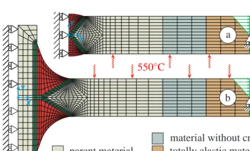
Figure 2: FE-meshes for type 1 (a) and type 2 (b) weldments with designation of different materials, boundary conditions and mechanical loading
and totally elastic material) representing reduced sets of parent material properties in the location of bending moment appli-cation avoids excessive stress concentrations in ratcheting and creep analysis. Both FE-models use ABAQUS element type CPE8R: 8-node biquadratic plane strain quadrilaterals with re-duced integration. The FE-meshes for type 1 and type 2 welds consist of 723 and 977 elements respectively.
Referring to the technical details [6, 7, 8, 9] the testing was performed at 550±3◦C under fully-reversed 4-point bending
with total strain ranges∆εtot of 0.25, 0.3, 0.4, 0.6 or 1.0% in the parent plate and hold periods∆t of 0, 1 or 5 hours using a
strain rate of 0.03%/s. For the purpose of shakedown and creep analysis using LMM, the conversion from strain-controlled test conditions to force-controlled loading in the simulations using bending moment M has been carried out and explained in [4].
Another effective analysis technique, successfully employed in [4], was to apply the bending moment M through the linear distribution of normal pressure P over the section of the plate as illustrated in Fig. 2 with the area moment of inertia in regard to horizontal axis X:
IX =w thk3/12, (7)
where the width of plate w=200 mm and the thickness of plate
thk=26 mm. Therefore, the normal pressure is expressed in terms of applied bending moment M and vertical coordinate
y of plate section assuming the coordinate origin in the
mid-surface:
P(y)=M y/IX. (8)
3. Plastic bending of plates
3.1. Solution with Ramberg-Osgood model
The cyclic stress-strain properties of the steel AISI type 316N(L) parent material and associated weld and HAZ met-als are presented in terms of the conventional Ramberg-Osgood equation and implemented in the LMM code for the creep-fatigue analysis [4]. The R-O model has the advantage that it can be used to accurately represent the stress-strain curves of metals that harden with plastic deformation, showing a smooth elastic-plastic transition at high temperatures:
∆εtot
2 =
∆σ 2 ¯E +
∆σ 2 B
!1/β
, (9)
where∆εtotis the total strain range;∆σis the equivalent stress range in MPa; B andβare plastic material constants; ¯E is the
effective elastic modulus in MPa defined as
¯
E= 3 E
2 (1+ν), (10)
where the Young’s modulus E in MPa and the Poisson’s ratioν are the uni-axial elastic material properties.
Although this relationship (9) is not explicitly solvable for stress range∆σ, an approximate solution for∆σcan be found using following recursive formulation:
∆σn+1
2 =B
∆εtot
2 −
∆σn
2 ¯E !β
with n≥3, (11)
where the initial iteration is defined as
∆σ0
2 =
∆εtot 2
!β
. (12)
For the case of plastic bending of a plate with a rectangu-lar cross-section, i.e. as was used in the experimental studies implemented by Bretherton et al. [6, 7, 8, 9], it is possible to formulate an analytic relation using the R-O material model for the applied bending moment M as proposed in [21]:
M=2 wσeop 3
thk
2
!2
1+3β+3 2β+1ε˜+
3 β+2ε˜
2
(1+ε˜)2
, (13)
where the maximum normal stress over a cross-section or
edge-of-plate stressσeop is defined based upon the plane strain as-sumption using equivalent stressσ
Table 2: The values of bending moment M obtained by Eqs (11-15) correspond-ing to the values of total strain range∆εtotfrom experiments [6, 7, 8, 9]
∆εtot, % 1.0 0.6 0.4 0.3 0.25
M,kN·m 10.068 7.924 6.368 5.347 4.739
and the ratio between plastic and elastic strains is formulated as
˜ ε=εpl
εel = ∆σ 2 B
!1/β
2 ¯E
∆σ. (15)
Other parameters of relation (13) include the material con-stants of the R-O model (β,B,E) and the geometric parameters¯
of a plate (thk and w). For the case of reverse bending tests of cruciform weldments at 550◦C implemented by Bretherton et
al. [6, 7, 8, 9], the total strain range∆εtotin outer fibre of parent material plate remote from weld was controlled to correspond to one of the required values. Knowledge of the stabilised cy-cle parent material properties of the steel AISI type 316N(L) described by the R-O model (9) reported in Table 1 of [4] and geometric parameters of specimen (thk=26 mm and w=200 mm) allows the calculation of the values of bending moments applied in experiments [6, 7, 8, 9] during the period of saturated cyclic response, as reported in Table 2.
Referring to [21], Eq. (13) gives a smooth variation of mo-ment with strain, which could be derived analytically employ-ing recursive formulas (11) and (12) for∆σdependent on∆εtot. Applying the recursive approach, the dependence of total strain range ∆εtot on applied moment M could be obtained. Firstly, Eq. (13) is inverted to recursive formula taking into account Eq. (14) as follows:
∆σn+1
2 =
M
4 w
3√3
thk
2
!2
1+3β+3 2β+1ε˜n+
3 β+2ε˜
2 n
(1+ε˜n)2
with ε˜n=
∆σn
2 B
!1/β 2 ¯E
∆σn
and n≥3,
(16)
where the initial iteration is defined as ∆σ0
2 =
M
2 w 3
2 √ 3
thk
2
!2 3
β+2
. (17)
Secondly, the conventional formulation of the R-O model (9) is applied to evaluate the total strain range∆εtot correspond-ing to the equivalent stress range obtained in Eqs (16) and (17). Such a useful relation for∆εtot(M) allows the estimation of an important control parameter of the LCF experiments, when the geometry of specimen is known and plastic deformation of a material is comprehensively described by the R-O model. Fig-ure 3 illustrates the application of both approaches (direct by Eqs (11-15) and inverted by Eqs (9, 16, 17)) to the parent ma-terial plate used in the experiments [6, 7, 8, 9] with particular dimensions of cross-section (thk =26 mm and w =200 mm) and particular material properties described by the R-O model (E=160 GPa,ν=0.3, B=1741.96 MPa,β=0.2996).
0 0.5 1.0 1.5 10
5
0
200mm
26mm
M M
steel 316N(L) at550ºC
12
total strain range (%)
b
en
d
in
g
m
o
m
en
t
(k
N
·
m
[image:5.612.29.277.391.545.2])
Figure 3: Curve presenting M vs.∆εtotrelationship for a parent plate with par-ticular cross-section and described by parpar-ticular R-O model material constants
3.2. Evaluation of limit load
It is desirable to convert the absolute values of bending mo-ment M into values of normalised bending momo-ment ˜M, which
is suitable for the formulation of an analytic assessment model for number of cycles to creep-fatigue failure N?, as proposed in [4]. Referring to [4] ˜M is defined as the relation of variable
bending moment range∆M to shakedown limit∆Msh: ˜
M= ∆M/∆Msh, (18)
where Msh is called initial yielding moment according to [21] and corresponds to the structural conditions, when yielding is just beginning at the edge of a beam.
The limit load and shakedown limit are evaluated with an elastic-perfectly-plastic (EPP) model and a von Mises yield condition using material properties corresponding to the satu-rated cyclic plasticity response (E,σyandν) reported in Table 1 of [4] for the steel AISI type 316N(L) at 550◦C.
In the case of a rectangular cross-section plate in bending, as-suming plane strain conditions (14), Mshis defined analytically according to [21] as
Msh=
σeop yw thk2
6 with σeop y=
2 √
3σy. (19)
The values of bending moment exceeding Msh with further growth of plastic strain gradually approach the limit load value or fully plastic moment, which is defined analytically [21] as
Mlim=σeop yw thk2/4. (20)
When M reaches the value of Mlim, it is assumed that the plate cross-section is completely in plastic flow leading to a
plastic hinge and structural collapse. It should be noted that
Table 3: The values of maximum normalised bending moment ˜Mmaxobtained numerically and corresponding to the configurations defined in Table 1
No. Configuration M˜max
type 1 type 2
1 Perfectly dressed 1.50906 1.51593
2 Typically dressed 1.54644 1.55124
3 Precisely as-welded 1.74042 1.78075
4 Typically as-welded 2.02637 2.05556
5 Coarsely as-welded 2.32326 2.30184
decreases, since the yielding starts at lower values of applied bending moment M comparing to whole plate, because of ma-terial and geometry non-uniformity. In [4], this ratio was called the maximum normalised bending moment
˜
Mmax= ∆Mlim/∆Msh, (21)
and it had a value of 1.551 for Type 2 dressed weldment [4]. Therefore, ˜Mmaxis dependent on the particular geometric con-figuration of the weldment, and therefore should be taken into account in the formulation of parametric relations. Following this assumption and Eqs (18) and (21) the normalised bending moment is introduced in the following form:
˜
M= M
Msh
= M ˜Mmax
Mlim
with Mlim=
σyw thk2 2√3
. (22)
Thus, the awareness of the parent material yield stress σy of the steel AISI type 316N(L) reported in Table 1 of [4] and geometrical parameters of specimen (thk = 26 and w = 200) allows the calculation of the limit bending moment as Mlim = 10.564 [kN·m] for the conditions of experiments [6, 7, 8, 9]. If the weld geometry is the same as in the cruciform weldment specimens, then ˜Mmax = 1.551 and the values of normalised bending moment ˜M in experiments [6, 7, 8, 9] are calculated as
reported in Table 4 of [4]. For other geometrical configurations of weldments, the set of ˜M will be slightly different, because
˜
Mmaxis individual for each geometrical configuration and were estimated numerically using step-by-step FEA.
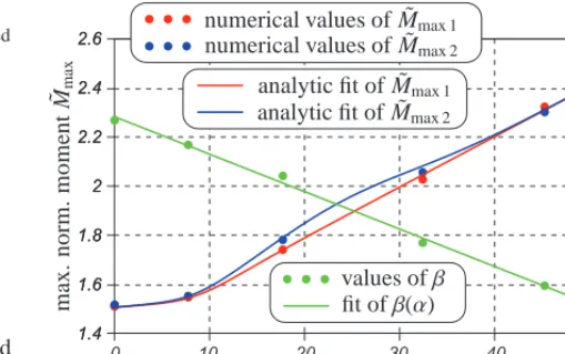
Table 3 lists the values of ˜Mmax corresponding to the geo-metric configurations defined in Table 1 for type 1 and 2 weld-ments. These values are calculated by Eq. (21), which includes the values of Mlimand Mshobtained numerically for each of the 10 configurations using step-by-step FEA with an EPP material model. Using the values of M from Table 2, the values of ˜Mmax reported in Table 3 and the value of Mlim = 10.564 [kN·m], the values of normalised moment ˜M for each configuration and
each∆εtotcan be calculated by applying Eq. (22). Thus, in or-der to provide the values of ˜M in fully analytical form, the
val-ues of ˜Mmaxhave to be defined as dependent on the geometric parameters of the weld profile (αandβ).
The maximum normalised moment ˜Mmax 1 for the type 1 weldment is dependent on angleαas follows
˜
Mmax 1(α)= f1(α) [1−H(α)]+f2(α) H(α) with f1(α)=m1α+m2, f2(α)=m3α+m4 and
H(α)=0.5+0.5 tanh α−m5
m6 !
.
(23)
0 10 20 30 40 50 2.6
2.4
2.2
2
1.8
1.6
1.4 2.6
2.4
2.2
2
1.8
1.6
1.4
60
50
40
30
20
10
0
numerical values of ˜Mmax 1 numerical values of ˜Mmax 2 analytic fit of ˜Mmax 1 analytic fit of ˜Mmax 2
angleα(◦)
m
ax
.
n
o
rm
.
m
o
m
en
t
˜ Mm
ax
values ofβ fit ofβ(α)
an
g
le
β
,
[image:6.612.44.255.56.144.2]◦
Figure 4: Numerical values of maximum normalised moment ˜Mmaxfrom Ta-ble 3 fitted by analytic approximations (23) and (24)
In notation (23) m1 = 0.00483 and m2 = 1.50906 are fit-ting parameters of the first linear part f1(α); m3=0.02062 and m4 = 1.37825 are fitting parameters of the second linear part f2(α); m5=8.28436 is the value ofαcorresponding to intersec-tion of funcintersec-tions f1(α) and f2(α) and m6 =5 is the smoothing parameter in an analytic approximation H(α) of the Heaviside step function. The result of fitting the ˜Mmax 1numerical values from Table 3 by the analytic function ˜Mmax 1(α) in the form of Eq. (23) is illustrated in Fig. 4.
Since the difference between values of ˜Mmaxfor types 1 and 2 corresponding to the same values ofαis relatively small, it can be concluded that the angleαhas a much more significant impact on the maximum normalised moment ˜Mmax 2 than the angleβfor the type 2 weldment. Moreover, the effect ofβon
˜
Mmax 2is limited to a quite narrow range of angles. Therefore, an optimal way to account for angleβis to fit the difference be-tween ˜Mmax 2and ˜Mmax 1from Table 3 with a Gaussian function dependent onβand produce a symmetric “bell” curve. In this case, the maximum normalised moment ˜Mmaxfor the types 1 and 2 weldments is dependent on anglesαandβ:
˜
Mmax(α, β)=M˜max 1(α)+m7exp
−m8β−m92
, (24)
where m7 = 0.06768 is the height of the curve’s peak, m8 = 0.01437 controls the width of the “bell”, and m9 = 25.995 is the position of the centre of the peak. To reduce the number of variables in Eq. (24), the angles ofαandβwere chosen so that their values formed a linear relation
β(α)=44.1451−0.76530α. (25)
Substitution of Eq. (25) into Eq. (24) means that ˜Mmaxis a func-tion ofαonly, as illustrated in Fig. 4.
4. Structural integrity assessments
4.1. Numerical creep-fatigue evaluation
Since the principal goal of the research is the formulation of parametric relations able to describe long-term structural in-tegrity of weldments, the creep-fatigue strength of each of the configurations from Table 1 should be evaluated in a wide range of loading conditions. These conditions are presented by dif-ferent combinations of∆εtotin the parent plate outer fibre, as a characteristic of fatigue effects, and duration∆t of dwell period,
as a characteristic of creep effects. The set of∆εtotvalues used are the same as in the experimental studies [6, 7, 8, 9], see Ta-ble 2. The set of∆t values used are the same as in the previous
simulation study [4]: 0, 0.5, 1, 2, 5, 10, 100, 1000 and 10000 hours. Therefore, for each of the 10 configurations 45 creep-fatigue evaluations must be performed with different values of ∆εtotand∆t. In order to estimate 450 values of number of cy-cles to failure N?, 450 FE-simulations of the parametric models
shown in Fig. 2 have been carried out, using the LMM method, material models and constants given in [4]. The outputs of the LMM have been processed by the creep-fatigue procedure pro-posed in [4] to evaluate N?, because it has been successfully
validated against experimental data [6, 7, 8, 9].
The concept of the proposed creep-fatigue evaluation proce-dure, considering time fraction rule for creep-damage assess-ment, is explained in detail in [4] and consists of 5 steps:
1. Estimation of saturated hysteresis loop using the LMM; 2. Estimation of fatigue damage using S-N diagrams; 3. Assessment of stress relaxation with elastic follow-up; 4. Estimation of creep damage using creep rupture curves; 5. Estimation of total damage using an interaction diagram.
Since the LMM requires lower computational effort com-pared to other methods, it appears to be an effective tool for ex-press analysis of a large number of different loading cases using automation techniques. In order to perform 450 FE-simulations in CAE-system ABAQUS and effectively retrieve 450 values of
N?, 3 analysis improvements using automation have been
de-veloped and applied in this parametric study.
The first automation technique is the embedding of all 5 steps of the proposed creep-fatigue evaluation procedure in FOR-TRAN code of user material subroutine UMAT containing the implementation of the LMM and material models described in [4]. For a detailed description of the numerical procedure for the creep strain and flow stress estimation in the LMM code refer to [5, 20], and for a general guide to the LMM imple-mentation using the ABAQUS user subroutines refer to [19]. The creep-fatigue evaluation procedure is implemented once the LMM has converged upon the stabilised cyclic behaviour. The LMM analysis was performed using three load instances in the cycle with creep dwell: 1) end of direct loading, 2) end of dwell period, 3) end of reverse loading. This results in a sat-urated hysteresis loop in terms of effective strain and effective von Mises stress for each integration point in the FE-model, as shown in Fig. 5 of [4]. The most important parameters (derived in the 1st step of the procedure) for further creep-fatigue evalu-ation are the total strain range∆εtot, stressσ1at the beginning
of dwell period and the elastic follow-up factor Z. These pa-rameters from each integration point with material properties for elasticity, fatigue and creep, defined in the ABAQUS in-put file, are transferred into a new subroutine. This subroutine implements the next 4 steps of the procedure [4], which calcu-lates and outputs the following parameters into ABAQUS result ODB-file: time to creep rupture t∗, creep damage accumulated
per cycleωcr
1c, number of cycles to fatigue failure N∗, fatigue damage accumulated per 1 cycleωf
1c, and the most important – total number of cycles to failure in creep-fatigue conditions
N?obtained using the damage interaction diagram proposed by
Skelton and Gandy [22]. It should be noted that this evaluation procedure was implemented in previous work [4] using Excel spreadsheets only for the most critical locations, identified man-ually as sites of∆εtotandσ1maximum values.
An example of the creep-fatigue evaluation procedure out-puts for the configuration no. 2 (typically dressed) of type 2 weldment corresponding to the loading case of∆εtot=1% and ∆t =5 hours is illustrated in Fig. 5. These results correspond to the FEA contour plots of the LMM outputs (obtained in Step 1) including∆εtot,εcr,ε
eq
vM at the beginning of dwell andε eq vM at the end of dwell, explained in [4] and illustrated there in Fig. 9. The critical location with N? = 279 cycles to failure
for this case is the corner element in the weld toe adjacent to HAZ. The distribution of pure creep damageωcr with maxi-mum valueωmax
cr = 0.294 at the critical location is shown in Fig. 5a. The distribution of pure fatigue damageωf with max-imum valueωmax
f = 0.375 at the critical location is shown in Fig. 5b. The distribution of total damageωtotwith maximum valueωmaxtot =0.669 at the critical location is shown in Fig. 5c. It should be noted that value ofωmaxtot doesn’t exceed 1, because the non-linear damage interaction diagram [22] is used in creep-fatigue evaluation. The distribution of N?with minimum value
Nmin? =279 at the critical location is shown in Fig. 5d.
Exactly the same approach is used to demonstrate an example of a type 1 weldment comprising geometry configuration no. 2 (typically dressed) and loading case of∆εtot = 1% and∆t = 5 hours. Figure 6 shows the outputs of FEA with the LMM, while Fig. 6 shows the outputs of the creep-fatigue evaluation procedure. The critical location with N?=206 cycles to failure
for this type 1 is the same as for the type 2 weldment – the corner element in the weld toe adjacent to HAZ.
The distribution of total strain range∆εtot, with maximum value ∆εmax
tot = 1.58 % at the critical location, is shown in Fig. 6a. The distribution of equivalent creep strainεcrat load instance 2 with maximum valueεcrmax =2.40953E-3 at the crit-ical location is shown in Fig. 6b. The distribution of equiv-alent von Mises stress σeqvM at the beginning of dwell at load instance 1 with valueσeq1 =334.743 MPa at the critical loca-tion is shown in Fig. 6c. The distribuloca-tion of equivalent von Mises stress σeqvM at the end of dwell at load instance 2 with valueσeq2 = 287.954 MPa at the critical location is shown in Fig. 6d. Therefore, the drop of stress∆σeq =46.789 MPa dur-ing∆t =5 hours of dwell provides the value of elastic follow up factor Z=7.25 at the critical location.
The distribution of pure creep damage ωcr with maximum valueωmax
2.723e+07 5.675e+06 1.368e+06 3.750e+05 1.159e+05 3.981e+04 1.510e+04 6.252e+03 2.805e+03 1.358e+03 7.015e+02 3.846e+02 2.228e+02 8.368e-01 4.826e-01 2.634e-01 1.360e-01 6.601e-02 2.990e-02 1.255e-02 4.848e-03 1.712e-03 5.478e-04 1.573e-04 4.014e-05 9.007e-06 4.905e-01 2.822e-01 1.547e-01 8.065e-02 3.968e-02 1.835e-02 7.936e-03 3.189e-03 1.185e-03 4.033e-04 1.252e-04 3.504e-05 8.782e-06 8.159e-01 4.022e-01 1.819e-01 7.477e-02 2.758e-02 9.038e-03 2.581e-03 6.330e-04 1.310e-04 2.238e-05 3.100e-06 3.365e-07 0 pure creep damage ωcr pure fatigue damage ωf creep-fatigue damage ωtot number of cycles to failure N?
a b c d
Figure 5: Contour plots of LMM results for type 2 weldment corresponding to∆εtot=1% on the outer fiber and∆t=5 hours of dwell, which lead to creep-fatigue failure in weld toe after 279 cycles: a) pure creep damageωcr; b) pure fatigue damageωf; c) creep-fatigue damageωtot; d) number of cycles to failure N?
1.862e−02 1.707e−02 1.552e−02 1.396e−02 1.241e−02 1.086e−02 9.307e−03 7.755e−03 6.202e−03 4.650e−03 3.098e−03 1.546e−03 0 2.845e−03 2.607e−03 2.370e−03 2.132e−03 1.894e−03 1.657e−03 1.419e−03 1.181e−03 9.433e−04 7.056e−04 4.679e−04 2.302e−04 0 359.018 328.958 298.898 268.838 238.778 208.719 178.659 148.599 118.539 88.479 58.420 28.360 0 307.895 282.089 256.283 230.477 204.670 178.864 153.058 127.252 101.445 75.639 49.833 24.026 0 total strain range ∆εtot equiv. creep strain εcr equiv. vM stress
σeqvM
(MPa)
equiv. vM stress
σeqvM
(MPa)
a b c d
Figure 6: Contour plots of LMM results for type 1 weldment corresponding to∆εtot=1% on the outer fiber of plate and∆t=5 hours of dwell: a) total strain range ∆εtot; b) equivalent creep strainεcr; c) equivalent von Mises stressεeqvMat the beginning of dwell; d) equivalent von Mises stressε
eq
vMat the end of dwell
9.870e-01 4.942e-01 2.266e-01 9.374e-02 3.460e-02 1.122e-02 3.146e-03 7.479e-04 1.476e-04 2.370e-05 2.992e-06 2.889e-07 0 5.532e-01 3.191e-01 1.749e-01 9.075e-02 4.425e-02 2.018e-02 8.568e-03 3.356e-03 1.205e-03 3.925e-04 1.156e-04 3.033e-05 7.029e-06 9.680e-01 5.596e-01 3.068e-01 1.577e-01 7.601e-02 3.395e-02 1.396e-02 5.246e-03 1.786e-03 5.443e-04 1.468e-04 3.466e-05 7.077e-06 2.673e+07 4.989e+06 1.099e+06 2.812e+05 8.222e+04 2.710e+04 9.954e+03 4.036e+03 1.786e+03 8.570e+02 4.426e+02 2.432e+02 1.419e+02 pure creep damage ωcr pure fatigue damage ωf creep-fatigue damage ωtot number of cycles to failure N?
a b c d
The distribution of pure fatigue damage ωf with maximum valueωmaxf =0.345 at the critical location is shown in Fig. 7b. The distribution of total damage ωtot with maximum value ωmaxtot = 0.668 at the critical location is shown in Fig. 7c. The distribution of N?with minimum value N?
min=206 at the criti-cal location is shown in Fig. 7d.
In spite of the same critical location and almost equal values of the accumulated total damage at failure for types 1 and 2 weldments, type 1 has less residual life caused by the increased values of parameters characterising the hysteresis loop (∆εtot, εcr,σeq
1 ,σ eq
2 and Z). Thus, one can conclude that geometrical parameterβhas a significant influence on N?.
The second automation technique is the development of a stand-alone application using Embarcadero Delphi inte-grated development environment using Delphi programming language. This simple application automatically carries out the sequence of all 45 FE-simulations with different M (cor-responding to ∆εtot according to Table 2) and ∆t values for
each of the configurations from Table 1. This is implemented by automated modification of the UMAT subroutine including changing of loading values (M and∆t) and output file names,
therefore producing 45 ABAQUS result ODB-files.
The third automation technique is the development of a script using ABAQUS Python Development Environment (Abaqus PDE) using Python programming language [23]. This simple script, when started in ABAQUS/CAE environment, appends the list of 45 ABAQUS result ODB-files corresponding to one configuration. For each of ODB-files, it reads the values of N? in each integration point, selects the integration point with min-imum value of N?over the FE-model, and writes the element number, integration point number and material name to an out-put text file. Therefore, the critical locations and corresponding values of N?are extracted automatically for all 450
configura-tions and loading cases. Obtained results can be used for the formulation of an analytic assessment model suitable for the fast estimation of N?for a variety of loading conditions ( ˜M and
∆t) and geometrical weld profile parameters (αandβ).
4.2. Analytic assessment model
For each of the 10 configurations from Table 1, the array of assessment results consisting of 45 values of N?
correspond-ing to particular values of ˜M and∆t is fitted using the least
squares method by the following function proposed in the form of power-law in [4]:
logN?=M˜−b(∆t)/a (∆t), (26)
where the fitting parameters dependent on dwell period∆t are a (∆t)=a3log (∆t+1)3+a2log (∆t+1)2
+a1log (∆t+1)+a0 and b (∆t)=b3log (∆t+1)3+b2log (∆t+1)2
+b1log (∆t+1)+b0,
(27)
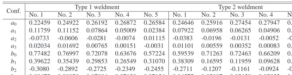
and the independent fitting parameters are reported in Table (4). In order to capture all configurations with an unified set of fitting parameters, parameters a0, a1, a2, a3, b0, b1, b2, b3from
Table 4 should be defined as dependent on geometric param-etersαandβusing the least squares method. For the type 1 weldments these parameters are dependent on angleαonly:
aT1
0 (α)=−4.175·10−
5α2+2.72
·10−3α+0.227, aT11 (α)=−2.169·10−3α+1.21
·10−1, aT1
2 (α)=1.907·10− 3α
−7.093·10−2, aT1
3 (α)=−5.352·10−
4α+1.968 ·10−2 bT10 (α)=−4.76324·10−3α+0.793, bT1
1 (α)=1.42·10− 4α2
−8.547·10−3α+0.4028, bT1
2 (α)=1.531·10− 3α
−0.3015, bT13 (α)=−3.08·10−4α+8.364
·10−2.
(28)
For the type 2 weldments these parameters include the de-pendence on angleαfrom Eqs (28) and an additional effect of angleβas in the following form:
aT2
0 (α, β)=a T1
0 (α)+3.179·10−
4β+2.355 ·10−3, aT2
1 (α, β)=a T1
1 (α)−1.636·10−
3β+3.043 ·10−2, aT22 (α, β)=aT12 (α)+1.636·10−3β
−3.043·10−2, aT2
3 (α, β)=a T1
3 (α)−4.136·10−
4β+7.33 ·10−3, bT2
0 (α, β)=b T1
0 (α)+0.0291
−1.684·10−4 exp(0.1622β), bT2
1 (α, β)=b T1
1 (α)−0.1789, bT2
2 (α, β)=b T1
2 (α)+0.1558, bT23 (α, β)=bT13 (α)−4.546·10−2.
(29)
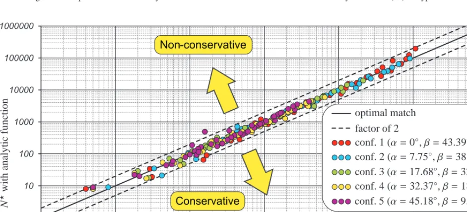
The verification of the fit quality using the the geometrical parameters (αandβ) for the proposed relations (28) and (29) is implemented by applying Eqs (26) and (27) to estimate N?. Number of cycles to failure N?is estimated for each of the 10 configurations using the corresponding values of angles from Table 1 and for the same load combinations as were used for the LMM analyses. The results of the verification are illustrated on diagrams in Fig. 8 for type 1 and Fig. 9 for type 2 weldments in the form of N?obtained with the analytic function (26) vs. N?
obtained with the LMM. Comparison of the analytic and nu-meric N?for both types of weldments shows that the quality of
Table 4: Sets of fitting parameters for Eq. (27) not dependent on∆t corresponding to configurations from Table 1
Conf. Type 1 weldment Type 2 weldment
No. 1 No. 2 No. 3 No. 4 No. 5 No. 1 No. 2 No. 3 No. 4 No. 5
a0 0.22459 0.24922 0.26192 0.26872 0.26584 0.24646 0.25916 0.27454 0.27947 0.27007
a1 0.11759 0.11152 0.07864 0.05009 0.02384 0.07922 0.06958 0.06265 0.04906 0.03958
a2 -0.0733 -0.0606 -0.0281 -0.0074 0.01115 -0.0383 -0.0196 -0.0131 -0.0052 -0.0035
a3 0.02034 0.01692 0.00765 0.00151 -0.0031 0.01101 0.00559 0.00352 0.00083 0.00032
b0 0.77482 0.76997 0.72078 0.63676 0.57224 0.59539 0.71263 0.72463 0.66209 0.60055
b1 0.39622 0.35439 0.29853 0.26549 0.31070 0.38309 0.16595 0.11959 0.09628 0.06507
b2 -0.3080 -0.2892 -0.2725 -0.2349 -0.2455 -0.2711 -0.1207 -0.1161 -0.0924 -0.0630
b3 0.08473 0.08028 0.07884 0.07130 0.07134 0.06572 0.02987 0.03439 0.03033 0.02533
of configuration no. 1 (perfectly dressed) is relatively the high-est among all configurations for both types of weldments. The average resistivity is slightly reducing from one configuration to another with the growth of angleαvalue as shown in Figs 8 and 9, resulting in the minimum average N?for the
configura-tion no. 5 (coarsely as-welded).
Having defined the number of cycles to failure N? by Eq. (26), the residual service life in years is therefore depen-dent on the duration of 1 cycle, which consists of dwell period ∆t and relatively short time of deformation as follows:
L?=N?
" ∆t
365·24+
2∆εtot( ˜M)
˙
ε(365·24·60·60)
#
, (30)
where ˙ε = 0.03%/s is a strain rate according to experimental conditions [6, 7, 8, 9], and the parametric analytical relations for ∆εtot( ˜M) are derived in Sect. 3. These relations consist of Eqs (9), (16) and (17) given in Sect. 3.1 to evaluate∆εtot(∆σ(M)), where M is replaced by ˜M and Mlimusing Eq. (22) and ˜Mmax using Eq. (24) given in Sect. 3.2. The aforementioned group of equations for the relation ∆εtot( ˜M) include the geometrical
parameters of parent plate cross-section (thk and w) and weld profile (αandβ), and parent plate material parameters (E,ν,
B, β, σy). This group of equations (9), (16), (17), (22) and (24) replaces Eq. (35) from [4], which is suitable for only one particular variant of weldment (type 2), weld profile (conf. 2 – typically dressed) and parent plate cross-section [6, 7, 8, 9].
5. Parametric formulation of FSRF
Since the function N?( ˜M,∆t) proved its validity in the
pre-vious subsection, it can be applied for the fast creep-fatigue assessments of new welded structures during the design stage. However, it is generally hard to generate conclusions about the service conditions ( ˜M,∆t) required to estimate particular value
of N?. Loading conditions comprise a wide range of mechani-cal loading described by ˜M or corresponding range of∆εtotin parent material adjacent to welded joints. Thus, introduction of a Fatigue Strength Reduction Factor (FSRF) allows a wide range of mechanical loading relevant to application area of a designed welded structure to be captured. The FSRF takes into account the difference in behaviour of the weldment compared to the parent material, considering weldments to be composed
of parent material. The FSRF is determined experimentally by comparing the fatigue failure data of the welded specimen with the fatigue curve derived from tests on the parent plate material. The current approach in R5 Volume 2/3 Procedure [10] op-erates with the fixed values of FSRF for 3 different types of weldments taking into account dressed and as-welded variants, which consider only the reduction of fatigue strength of weld-ments compared to the parent material. For austenitic steel weldments [24, 25], FSRF =1.5 is prescribed for both vari-ants of type 1, and FSRF=1.5 for type 2 dressed and FSRF= 2.5 for as-welded variant. All this variety of the FSRFs is rep-resentative of the reduction in fatigue endurance caused by the local strain rangeεtotenhancement in the weldment region due to the material discontinuity and geometric strain concentration effects. The introduction of FSRF as dependent on∆t in [4]
us-ing function N?( ˜M,∆t) for the case of type 2 dressed weldment
allowed the influence of creep to be taken into account, and to provide the adjusted values of FSRF for the real operation conditions, where creep-fatigue interaction takes place. There-fore, the same approach [4] is applied to obtain∆t-dependent
FSRFs for a variety of geometrical configurations considering additional dependence on parameters of weld profile (αandβ). For this purpose Eq. (26) is converted analytically to the rela-tion ˜M(N?,∆t) and inserted into the group of relations∆εtot( ˜M)
given in the end of previous subsection, resulting in the relation ∆εtot(N?,∆t, α, β). This relation describes the∆εtotin the par-ent material remote from weldmpar-ent corresponding to particular values of N? and∆t for a particular geometrical configuration
of weldment defined byαandβ. Thus, the FSRFs, appropri-ate to varying values of∆t and equal values of N?, are defined
by the relation between the S–N diagram corresponding to fa-tigue failures of parent material plate and S–N diagrams for a weldment defined byαandβ:
FSRF= ∆εpartot(N?)/∆εtot(N?,∆t, α, β), (31) where the S–N diagram for parent material plate is defined as
log∆εpartot=p0+p1 log (N∗)+p2 log (N∗)2, (32) with the following polynomial coefficients referring to [25]:
p0=2.2274, p1=−0.94691 and p2=0.085943.
1 10 100 1000 10000 100000 1000000
1 10 100 1000 10000 100000 1000000
Non-conservative
Conservative
Number of cycles to failure N?with the LMM
N
?
w
it
h
an
al
y
ti
c
fu
n
ct
io
n
optimal match
factor of 2 conf. 1 (α=0◦)
conf. 2 (α=7.75◦)
conf. 3 (α=17.68◦)
conf. 4 (α=32.37◦)
[image:11.612.57.523.30.235.2]conf. 5 (α=45.18◦)
Figure 8: Comparison of number of cycles to failure N?obtained with the LMM and the analytic function (26) for type 1 weldment
1 10 100 1000 10000 100000 1000000
1 10 100 1000 10000 100000 1000000
Non-conservative
Conservative
Number of cycles to failure N?with the LMM
N
?
w
it
h
an
al
y
ti
c
fu
n
ct
io
n
optimal match
factor of 2
conf. 1 (α=0◦,β=43.39◦)
conf. 2 (α=7.75◦,β=38.38◦)
conf. 3 (α=17.68◦,β=32.08◦)
conf. 4 (α=32.37◦,β=18.42◦)
[image:11.612.52.523.273.486.2]conf. 5 (α=45.18◦,β=9.65◦)
Figure 9: Comparison of number of cycles to failure N?obtained with the LMM and the analytic function (26) for type 2 weldment
11
10
9
8
7
6
5
4
3
2
1
0.01 0.1 1 10 100 1000 10000 0.01 0.1 1 10 100 1000 10000 11
10
9
8
7
6
5
4
3
2
1
a b
dwell time (hours) dwell time (hours)
F
S
R
F
F
S
R
F
Configurations: Configurations:
1. Perfectly dressed 1. Perfectly dressed
2. Typically dressed 2. Typically dressed
3. Precisely as-welded 3. Precisely as-welded
4. Typically as-welded 4. Typically as-welded
5. Coarsely as-welded 5. Coarsely as-welded
[image:11.612.48.525.524.678.2]Table 5: The values of FSRFs for pure fatigue for types 1 and 2 weldments corresponding to the configurations from Table 1
Conf. 1 2 3 4 5
Type 1 1.146 1.444 2.062 2.896 3.308
Type 2 1.362 1.682 2.372 3.137 3.430
N?. This range is different for each value of∆t characterised
by reducing value of the average N?with the growth of∆t. The
upper bound of the N?range is governed by the mathematical
upper limit of the S–N diagram∆εpartot(N?) for parent material
plate, which is defined in [4] as log(N?
max) = p1/(2 p2)=5.51 or∆εpartot(105.51)=0.416%. The lower bound of the N?range is
flexible and governed by∆t using the following function:
logNmin? =3−0.5 log (∆t+1). (33)
Finally, for each of the 10 configurations from Table 1 the FSRF is defined as a continuous function of∆t using Eq. (31)
using simple averaging procedure over a dynamic range of N? from logN?
min
to log N? max
with step 0.01. The resultant
de-pendencies of FSRFs on∆t are illustrated in Fig. 10a for type
1 and in Fig. 10b for type 2 weldments with designation of dif-ferent configurations. First of all, these figures show signifi-cant enhancement of FSRF for dwells ∆t > 0.1 hour caused by creep, which is important for design applications. The ini-tial values of FSRFs corresponding to pure fatigue conditions (∆t =0) are listed in Table 5 and could be compared with the values recommended in R5 Volume 2/3 Procedure [10].
The FSRF for type 1 dressed weldments is within the range 1.146–1.444 depending on the quality of grinding, while R5 gives the value 1.5 (refer to [24, 25]), which is more conser-vative. The FSRF for type 1 precisely welded joints with-out grinding is within the range 1.444–2.062 depending on the quality of welding, while R5 gives the same value 1.5, which is non-conservative. The FSRF for type 1 coarsely welded joints without any additional treatment may reach up to 3.308, while R5 doesn’t give any value for this case.
The FSRF for type 2 dressed weldments is within the range 1.362–1.682 depending on the quality of grinding, while R5 gives the value 1.5, which approximately corresponds to aver-age value for the obtained range. The FSRF for type 2 precisely welded joints without grinding is within the range 1.682–2.372 depending on the quality of welding, while R5 gives the value 2.5, which is more conservative. The FSRF for type 2 coarsely welded joints without any additional treatment may reach up to 3.43, while R5 doesn’t give any value for this case.
Using the proposed approach in this work, the values of FS-RFs reported in Table 5 could be easily revised, if the ranges of angles αandβcharacterising the quality of weldment are modified. It should be noted that the FSRF of 1.682 for type 2 dressed weldment revises the value of 1.77 reported in previous work [4], because the form of fitting functions (26) and (27) has been improved in this work providing less conservatism in N?
predictions for pure fatigue.
6. Conclusions
The parametric study on creep-fatigue strength of the steel AISI type 316N(L) weldments of types 1 and 2 according to classification of R5 Vol. 2/3 Procedure [10] at 550◦C has been
implemented using the LMM. The study is based upon the latest developed creep-fatigue evaluation procedure [4] considering time fraction rule for creep-damage assessment. This procedure has been successfully validated in [4] against experimental data [6, 7, 8, 9] comprising reverse bending tests of cruciform weld-ments for different combination of loading conditions (dwell period∆t and normalised bending moment ˜M).
Parametric models of geometry and FE-meshes for both types of weldments shown in Figures 1 and 2 are developed in a way which allows variation of parameters governing shape of the weld profile (anglesαandβ) and loading conditions (∆t
and ˜M). Five configurations, characterised by individual sets of
parameters listed in Table 1, are proposed to present different fabrication cases and to characterise weldment manufacturing quality. For each of configuration, the total number of cycles to failure N? in creep-fatigue conditions is assessed
numeri-cally for different loading cases using several LMM-analysis automation techniques described in Sect. 4.1. The obtained set of N?is extrapolated by the analytic function (26) dependent on
˜
M with fitting functions (27) dependent on∆t, which includes
the fitting parameters (28) and (29) dependent on geometrical parameters (αandβ). The difference in analytical predictions compared to LMM-based assessment is that the results for pure fatigue are relatively conservative, but are still within the factor of 2 allowed by engineering standards, as shown in in Fig. 11.
Proposed function (26) for N? shows good agreement with
numerical results obtained by the LMM in Figures 8 and 9 for types 1 and 2 weldments correspondingly. The discrepancy be-tween analytic predictions and numerical LMM outputs is gen-erally found to be within the boundaries of an inaccuracy factor equal to 2, which is allowable for engineering analysis, produc-ing both conservative and non-conservative results. Therefore, it is used for the identification of FSRFs intended for design purposes and dependent on∆t and geometrical parameters (α andβ). The proposed function for FSRFs (31) is applied to all 10 configuration from Table 1 characterised byαandβin or-der to obtain continuous dependencies on∆t, which are shown
in Figures 10a and 10b for types 1 and 2 weldments respec-tively. Therefore, this approach improves upon existing design techniques, e.g. in R5 Procedure [10], by considering the sig-nificant influence of creep. Moreover, the obtained FSRFs for pure fatigue revises the values recommended in R5 Procedure [10] removing the redundant conservatism for type 1 dressed weldments and type 2 undressed weldments.
Finally, in order to conclude about the global sensitivity of creep-fatigue strength to a change of parameters, the set of equations (26) – (29) for N?( ˜M,∆t, α, β) are applied to create
a set of contour plots shown in Fig. 11. These plots charac-terise the influence of geometric parameters (αandβ) on N?
at 4 different combinations of loading conditions (∆t and ˜M)
1995 1778 1585 1413 1259 1122 1000 891 794 708 631 562 501 447 398 355 316 282 251 224 200 178 158 141 126 112 100 0 5 10 15 20 25 30 35 40 45 50
50 45 40
35 30 25 20 15 10 5 0
0 5 10 15 20 25 30 35 40 45 50 50
45 40 35 30 25 20
15 10 5 0
0 5 10 15 20 25 30 35 40 45 50 50
45 40 35 30 25 20
15 10 5 0
0 5 10 15 20 25 30 35 40 45 50 50
45 40
35 30 25 20 15 10 5 0
angleα◦
angleα◦
angleα◦
angleα◦
an
g
le
β
◦
an
g
le
β
◦
an
g
le
β
◦
an
g
le
β
◦
dwell period∆t
n
o
rm
al
is
ed
m
o
m
en
t
˜ M
˜
M=1.0, ∆t=10h
˜
M=1.0, ∆t=100h ˜
M=1.5, ∆t=10h
˜
M=1.5, ∆t=100h
[image:13.612.65.509.27.331.2]cycles to failure N?
Figure 11: Contour plots for type 2 weldment characterising the influence of geometric parameters (αandβ) on number of cycles to failure N?for different combinations of loading conditions (∆t and ˜M) obtained with Eqs (26) – (29)
these effects are dependent on intensity of mechanical load ˜M
and length of dwell period∆t. The growth of∆t changes the
positive influence ofβto negative and smoothes the negative influence ofαon N?. The growth of ˜M changes the negative
influence of αto positive and smoothes the positive influence ofβon N?. The intensity of a parameter (αorβ) influence is characterised by the relative density of contour edges crossing the corresponding axis. Since both parameters can not increase their values simultaneously, only half of each plot, including upper left, lower left and lower right corners, is of importance. Figure 11 shows that the change of both loading parameters (∆t and ˜M) quite significantly changes the location of contour
edges, and therefore the contribution ofαandβon N?.
Further research is devoted to parametric study on creep-fatigue strength of Type 3 weldment, which includes the vari-able distance between welded parts l as the 3rd geometric pa-rameter along with αandβ. The function for N? should be
extended to account for the effect of l based upon the numerical results using LMM for different configurations. This will allow consideration of the effect of l on the∆t-dependent FSRF for
Type 3 dressed and as-welded variants, which has the value of 3.2 for pure fatigue prescribed in R5 Vol. 2/3 Procedure [10].
Acknowledgements
The authors deeply appreciate the Engineering and Physical Sciences Research Council (EPSRC) of the UK for the financial
support in the frames of research grant no. EP/G038880/1, the University of Strathclyde for hosting during the course of this work, and EDF Energy for the experimental data.
References
1. Lee, Y.-L., Barkey, M.E., Kang, H.-T.. Metal Fatigue Analysis
Hand-book: Practical Problem-Solving Techniques for Computer-Aided Engi-neering. Oxford: Butterworth-Heinemann; 2012.
2. Radaj, D., Sonsino, C.M., Fricke, W.. Fatigue Assessment of Welded
Joints by Local Approaches. Cambridge: Woodhead Publishing Limited;
2nd ed.; 2006.
3. Łagoda, T.. Lifetime Estimation of Welded Joints. Berlin: Springer-Verlag; 2008.
4. Gorash, Y., Chen, H.. Creep-fatigue life assessment of cruciform weldments using the linear matching method.
Int J of Pressure Vessels & Piping 2012;:14 p., Manuscript no. IPVP3257, in press, DOI: 10.1016/j.ijpvp.2012.12.003, https://docs.google.com/open?id=0Bx4lucS7z9cpNC1ZX2V3REk0em8. 5. Chen, H.F., Chen, W., Ure, J.. Linear matching method on the evaluation of cyclic behaviour with creep effect. In: Proc. ASME Pressure Vessels&
Piping Conf. (PVP2012). Toronto, Canada: ASME; 2012, July 15-19.
6. Bretherton, I., Knowles, G., Slater, I.J., Yellowlees, S.F.. The fatigue and creep-fatigue behaviour of 26mm thick type 316L(N) welded cruci-form joints at 550◦C: An interim report. Report for Nuclear Electric Ltd
no. R/NE/432; AEA Technology plc; Warrington, UK; 1998.
7. Bretherton, I., Knowles, G., Bate, S.K.. PC/AGR/5087: The fatigue and creep-fatigue behaviour of welded cruciform joints: A second interim report. Report for British Energy Generation Ltd no. AEAT-3406; AEA Technology plc; Warrington, UK; 1999.
![Figure 1: Designations of parameters fully describing weld profile geometriesof types 1 and 2 weldments and applied bending moment, according to [6]](https://thumb-us.123doks.com/thumbv2/123dok_us/1661457.119702/2.612.293.542.24.335/figure-designations-parameters-describing-prole-geometriesof-weldments-according.webp)
![Table 2: The values of bending moment Ming to the values of total strain range obtained by Eqs (11-15) correspond- ∆εtot from experiments [6, 7, 8, 9]](https://thumb-us.123doks.com/thumbv2/123dok_us/1661457.119702/5.612.294.546.21.149/table-values-bending-moment-values-obtained-correspond-experiments.webp)