The reliability of diverse systems: a contribution using modelling of the fault creation process

City, University of London Institutional Repository

Citation:

Popov, P. T. & Strigini, L. (2001). The reliability of diverse systems: a contribution using modelling of the fault creation process. Paper presented at the International

Conference on Dependable Systems and Networks, 1 - 4 Jul 2001, Goteborg, Sweden.

This is the unspecified version of the paper.

This version of the publication may differ from the final published

version.

Permanent repository link:

http://openaccess.city.ac.uk/258/

Link to published version:

Copyright and reuse: City Research Online aims to make research

outputs of City, University of London available to a wider audience.

Copyright and Moral Rights remain with the author(s) and/or copyright

holders. URLs from City Research Online may be freely distributed and

linked to.

City Research Online: http://openaccess.city.ac.uk/ [email protected]

Peter Popov (corresponding author), Lorenzo Strigini Centre for Software Reliability, City University

Northampton Square, London, EC1V 0HB, UK

phone: +44 (0)20 7477 8963, fax: +44 (0)20 7477 8585

e-mail: (ptp,strigini)@csr.city.ac.uk

Version: 25 January, 2001

CSR technical report - submitted for publication

Abstract

Design diversity is a defence against design faults causing common-mode failure in

redundant systems, but we badly lack knowledge about how much reliability it will buy in

practice, and thus about its cost-effectiveness, the situations in which it is an appropriate

solution and how it should be taken into account by assessors and safety regulators. Both

current practice and the scientific debate about design diversity depend largely on intuition.

More formal probabilistic reasoning would facilitate critical discussion and empirical

validation of any predictions: to this aim, we propose a model of the generation of faults

and failures in two separately-developed versions. We show results about: i) what degree

of reliability improvement an assessor can reliably expect from diversity; and ii) how this

reliability improvement may change with higher-quality development processes. We

The Reliability of Diverse Systems: a Contribution

using Modelling of the Fault Creation Process

Peter Popov , Lorenzo Strigini

1. Introduction

Design diversity is an intuitively attractive method for increasing the reliability of critical

systems, including critical software, subject to design error. However, its use is

controversial because we do not know how to quantitatively evaluate its advantages. So, a

system designer does not know precisely how cost-effective diversity will be, compared to

other methods for improving system dependability, and generally safety assessors and

regulators do not know how effective it has been, in a system that they are called to

evaluate.

Design diversity requires that each redundant computation channel run a separate version

(or "variant") of the software, developed by a separate team, without communication

between the teams, to avoid the propagation of any errors between the teams. Other

precautions may be added ("forced" diversity) for minimising the chance of

common-cause errors in the design process: for instance, different principles of operation for the

two channels, different design methods, notations, and computer-aided design tools.

Experimental evaluation of the advantages from design diversity is severely limited.

Real-world diverse systems usually suffer too few failures of their component versions to give

any precise indication of the gain produced by diversity; controlled experiments are limited

by cost to being inadequate replicas of an industrial development process.

Practical decisions about whether to use diversity, how to apply it in a project, and how to

assess its effect on the dependability of the resulting system, are thus based on

industry-specific traditions, on intuition and on speculation. So, design diversity remains

controversial, although its use is practically mandatory in some industries. Opponents

claim that its benefits are limited and similar benefits could be achieved, with fewer

negative effects on cost and project complexity, by better engineering of a single software

version. Supporters object that these claims are unproven and diversity is an obviously

advantageous, feasible method. Such arguments cannot be resolved rationally without an

agreement on how to estimate how much benefit diversity will bring in a given situation.

achieved by multiple-version software, Hatton [1] offers a tentative argument based on: 1)

the reliability advantage given by diversity in the Knight-Leveson experiment [2], and 2)

the fact that, if versions failed independently, increasing the reliability of the versions

would also increase the reliability gain given by diversity. Extrapolating from these facts

he concludes that the balance of evidence points to diversity as better than alternative

methods for achieving high reliability. Though useful as a "what if" projection to stimulate

debate, this way of reasoning implicitly treats the specific measures chosen for

mathematical convenience as physical invariants, without proposing any plausible,

empirically verifiable (or, rather, falsifiable) causal model that would give them this status.

We set out to improve on these previous discussions by modelling the effect of diversity

in terms of a more concrete model of the mechanisms that are believed to produce them. In

this, we follow the approach of Eckhardt and Lee [3] and Littlewood and Miller [4] (both

summarised in [5]. In the rest of the paper, we will refer to their models as the "EL" and

"LM" models, for brevity), which produced convincing arguments against beliefs in failure

independence between diverse versions, and intuition about the factors that make diversity

more effective. However, the entities in our model are closer to observable entities in

software development, and we try to predict measures of more practical interest than the

mean probability of failure1 _{studied in these earlier papers.}

We limit our discussion to a very simple scenario, which yet has important practical

applications:

- we consider "non-forced" diversity, pursued by only enforcing strict separation

between the developments of the two versions. This is the situation in some actual

software projects, but in addition it can be seen as a worst-case analysis for the many

real systems in which "forced" and "functional” diversity are used. These are

expected to be superior to non-forced diversity, but the degree of superiority is

unknown: hence the utility of studying a limiting case;

- we consider the simplest possible diverse-redundant configuration: two versions, with

perfect adjudication (simple "OR" combination of binary outputs, giving a

"1-out-of-2", diverse system). This configuration has important practical applications, e.g. in

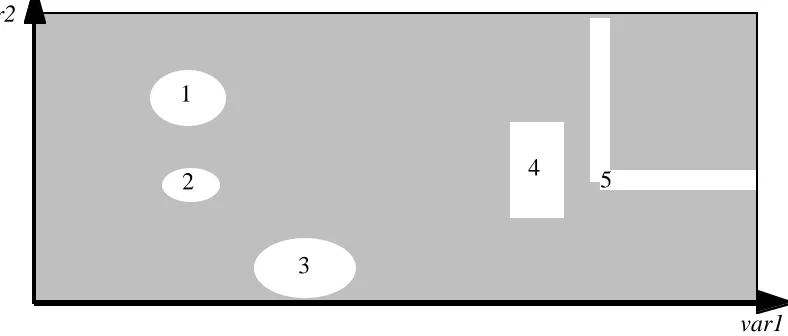
plant protection systems (Fig. 1).

1 _{The mean is taken over the population of all versions which could have been written, under the same known}

Protection system

Channel 1

Channel 2

Sensed plant state variables

Plant

[image:5.595.106.489.84.293.2]

Parallel (OR, 1-out-of-2) actuators for shut-down

Fig. 1 Dual-channel, 1-out-of-2 protection system: stylised view. In reality, the

two channels usually sense different state variables and may use different

actuators for shutting down the plant. We study the limiting worst case in

which this functional diversity does not apply. We argued in [8] why

functional diversity should be studied as part of a continuum of diversity

arrangement, rather than a radically different form.

In Section 2, we describe the model we use. In Section 3, we study its implications, asking

two questions:

- what amount of gain does the model predict from using diversity? This question is

relevant for assessors (e.g. in regulatory agencies for safety-critical systems) who

have to decide whether a specific diverse system is dependable enough for operation;

and to project managers in the choice of development methods;

- should we then expect the advantages procured by diversity to increase or to decrease

with increasing quality of the development process (interpreted as average reliability

of the versions)? This question concerns the evolution of development processes, and

in the short term it concerns the many software development organisations which

need to evolve their processes to face increasingly stringent dependability

requirements. Deciding this question may involve, in extreme cases, abandoning

diversity as a consequence of adopting other dependability-enhancing strategies, or,

vice-versa, adopting diversity rather than alternative improvement strategies. Many

believe that the better the versions, the higher the gain from fault tolerance, on the

In Section 3, we study the implications of this model in general. We observe that useful

qualitative conclusions can be drawn if we separate two extreme cases: that of very

high-quality software with a high chance of having no faults (discussed in Section 4), and that

of software in which very many, but low-probability faults are possible (discussed in

Section 5). Our summary and discussion of results is in Section 6.

2. Our model

2.1. Failure points and failures

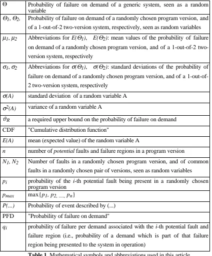
Consider the demand space2_{, i.e., the set of all possible demands on the 2-channel system.}

A demand occurs when the controlled system enters a state that requires the intervention of

the protection system. Demands differ in the details of the state of the controlled system,

and thus possibly in the input sequences that they cause to the protection system. A design

fault in a version consists in the fact that, for one or more possible demands, that version

will not respond as required (it will fail). Any such demand is a failure point in the

demand space for that version. Any set of demands on which a version will fail is called a

failure region for that version. If a failure region of one version overlaps with a failure

region of the second version, their intersection is a failure region for the system: demands

from this region will cause the two-version system to fail.

2 _{Called the input space in previous literature. We use the term "demand space" because we have found}

1

4 2

3

5

[image:7.595.106.500.111.279.2]

var1 var2

Fig. 2. An example of failure regions in a two-dimensional demand space:

each demand is a single reading of two input variables, var1 and var2. Various

authors have reported the shapes of failure regions in actual programs with

multi-dimensional demand spaces [9, 10, 11]. Besides simple shapes like

those shown above, they have found intuitive shapes, including

non-connected regions like arrays of separate points or lines.

Each demand in the demand space has a certain (possibly unknown) probability of

happening during the operation of the controlled system. If we add up the probabilities of

all those demands that are failure points for both versions, we obtain the probability of

failure on demand (PFD) of the two-version protection system.

This is essentially the basis of the models used in [3] and [4] .

2.2. Faults and their introduction

We know from experience that a mistake in design will not usually affect a single point in

the demand space, but a whole set. If the mistake is made, the whole set of points becomes

a failure region; if not, the failure region will not be there.

So, our simple model considers that there is a fixed set of possible faults, each one with its

associated failure region, and each corresponding to one of the mistakes that may be

made. A mistake, here, is a mistake of the whole development process, so that a fault is left

in the delivered product: it includes a whole sequence of human errors, first in the act of

unnoticed, or to be only partially fixed3_{. The accidental errors in the development process}

select some of these faults, at random. Some faults are more likely than others to be

chosen; some failure regions are "larger" than others, in the sense that the probability that

a demand will be in these regions is higher. Developing versions for a given application

under a regime of separate development means choosing, randomly and independently,

possible subsets of this set of possible faults4_.

We thus have a collection of potential faults and associated failure regions, {F₁, F₂, ...,

F_n}. Each one, e.g., F_i, has a certain probability p_i of being actually produced in a newly

developed version (following [3], [4] again, we can think of the process of producing a

version as sampling from a distribution of possible versions). It is also characterised by its

probability q_i, of being 'hit' during operation, i.e., its contribution to the unreliability of the

system.

We assume these failure regions to be non-overlapping. So, the PFD of a version is given

by the sum of the q_i values of those faults that are actually present.

So far, this model is the same as the EL and LM models, except in being

"coarser-grained": we consider whole failure regions rather than individual failure points. The

conclusions of the EL and LM models about the average PFD of a two-version system

(greater than the product of the versions' average PFDs) are easily re-derived here.

However, the average reliability is not especially interesting in practical decision-making:

we need some idea of the probability of achieving a given reliability, i.e., about probability

distributions rather than averages. Such predictions cannot be obtained from the EL and

LM models, because their parameters do not describe how likely it is that a version has a

certain set of failure points or failure regions: they only describe each failure point in

isolation. We need to add some further information to the model: we add the assumption

that the mistakes are statistically independent of each other. It is as though the design team,

faced with the possibility of inserting a fault, tossed dice to decide whether to insert it or

not.

3 _{The concept of a "fault" corresponding to each failure region is unnecessary for this model, and the term}

"fault" itself is loaded with implicit, unrealistic assumptions (cf [12]), but we use it here as a convenient simplification. Thus, "the th fault is present in version A" is a convenient short-hand for "in version A, the i-th potential failure region is actually a failure region".

4 _{It may be useful to recall here that assuming "independent choice" does not imply that the versions will fail}

All these additional assumptions - one-to-one mapping between faults and failure regions,

non-overlapping failure regions, and independent introduction of faults - which,

incidentally, are shared by most other models of software failure processes in the

literature - are obviously false. However, 1) we believe that they do not make a big

difference on the main useful results of the model, and will argue this thesis later; and 2) it

is much easier to check and refute empirically whether they are acceptable approximations

of reality than it was for the assumptions used in previous arguments about diversity. So,

we ask the reader to accept them and follow us in examining the implications of this

Θ Probability of failure on demand of a generic system, seen as a random variable

Θ1, Θ2, Probability of failure on demand of a randomly chosen program version, and

of a 1-out-of-2 two-version system, respectively, seen as random variables

µ1, µ2 Abbreviations for E(Θ1), E(Θ2): mean values of the probability of failure

on demand of a randomly chosen program version, and of a 1-out-of-2

two-version system, respectively

σ1, σ2 Abbreviations for σ(Θ1), σ(Θ2): standard deviations of the probability of

failure on demand of a randomly chosen program version, and of a

1-out-of-2 two-version system, respectively

σ(A) standard deviation of a random variable A

σ2_(A) variance of a random variable A

ϑR a required upper bound on the probability of failure on demand

CDF "Cumulative distribution function"

E(A) mean (expected value) of the random variable A

n number of potential faults and failure regions in a program version

N₁, N₂ Number of faults in a randomly chosen program version, and of common

faults in a randomly chosen pair of versions, seen as random variables

p_i probability of the i-th potential fault being present in a randomly chosen

program version

p_max max{p₁, p_{2, ....,} p_n}

P(...) Probability of event described by (...)

PFD "Probability of failure on demand"

q_i probability of failure per demand associated with the i-th potential fault and

failure region (i.e., probability of a demand which is part of that failure

[image:10.595.80.504.84.595.2]

region being presented to the system in operation)

Table 1. Mathematical symbols and abbreviations used in this article

3. The PFD of one-version and of two-version systems

In this model, the PFD for a version or system is the sum of many independent random

variables, i.e., the contributions of the individual potential faults. The mean and the variance

of this sum are then equal to the sums of the means and of the variances of the individual

random variables, respectively. The i-th random variable takes the value q_i with probability

probabilities become p_i2 _{and (1-pi}2 _{) for a two-version system, since we consider}

independent developments of the two versions. Thus:

E p qi i

i n

[Θ1]

1

=

=

∑

, _E

( )

_{p q}

i i i

n

[Θ2]

2

1

=

=

∑

, (1)

(

)

σ(Θ1)

2 1

1

= −

=

∑

pi p qi i i

n

, σ(Θ2)

(

)

2 2

1

2

1

= −

=

∑

pi pi q

i n

i (2)

Given n potential faults, we have a model with 2n parameters. All parameters are unknown

and unmeasurable in practice. So, direct use of these formulas is out of the question.

Despite this, we now proceed to use this model in a way that has practical value, by

selecting special cases of interest in which the study of the model is simple and does not

require detailed knowledge of all parameters. We consider two measures of reliability,

which have practical relevance in different scenarios. These are at the two ends of a

spectrum of possible scenarios:

- some programs (e.g. in some safety systems) are very simple and developed to high

standards: it is plausible that they often contain no fault. The expected value of the

number of faults is close to 0, and all the p_i are close to 0. There are only two events

with non-negligible probability: having zero common faults or having one common

fault. However, even one fault (common to the two versions) may be enough to violate

the system dependability requirements. So, we are effectively interested in the

probability of the versions having no common fault.

- there are very many possible faults, and many have small q_i compared to the

acceptable system PFD. We are then interested in the probability of the system PFD

not exceeding a required bound ϑ_R, or vice-versa in which bound will not be

exceeded with a set probability. E.g., we might ask what is the 99th percentile of the

distribution of the system PFD (i.e., an upper bound such that the system PFD has

99% probability of not exceeding it). For this scenario, we will exploit the fact that the

PFD of our systems is a sum of independent variables to approximate the distribution

of the PFD with a normal (Gauss) distribution, according to the central limit theorem.

As this is an asymptotic result, we will not know in practice how good an

approximation it is in a specific case, but this simplification is useful for studying the

3.1. Lemmas: considerations on the means and standard deviations of the PFD

We briefly study these measures, in part to be able to compare our observations with

previous studies, but more importantly to derive useful lemmas for the rest of the analysis.

3.1.1. Comparison between the mean PFDs, µ 1 and µ 2

As indicated above,

µ1 1

=

=

∑

p q_{i i}

i n

, µ2

2 1

=

=

∑

p q_{i i}

i n

(3)

We now define p_max=max{p₁, p_{2, ....,} p_n}. We can thus write:

µ2 µ

2

1 1 1

1

= ≤ = =

= = =

∑

p qi i

∑

p p q p

∑

p q p

i n

i i i

n

i i i

n

max max max (4)

Quality assurance activities strive to reduce the values of the p_i parameters. The actual

values are not known. However, these parameters have intuitive meanings relating to

developers' experiences, and the typical values achieved by given software development

processes could be studied empirically. Estimating small p_i parameters could be

infeasible, but to use inequality (4) we only need to estimate an upper bound.

So, if an assessor were convinced that a developer’s quality assurance activities reduce the

probability of the most common fault to, say, 10%, the assessor should also believe that a

two-version system from that developer has, on average, at least 10 times better PFD than a

single version. This may be a modest reliability gain, in particular compared with claims of

independence (for this upper-bound prediction to be equivalent to or better than

independence, we would need p_max ≤ µ1), but is an indisputable upper bound (on the

average unreliability).

3.1.2. Comparison between the standard deviations of the PFD, σ 1 and σ ₂

We have seen in (2) that:

σ2 1

1

2

1

Θ

( )

=

(

−

)

=

∑

p_i p q

i n

i i (5)

σ2 2

2 1

2 2

1

Θ

( )

=

(

−

)

=

∑

p_i p q

i n

i i (6)

p2(1-p2)≤p(1-p), iff p≤ (-1+50.5)/ 2= 0.618033987

So, if we write:

( )

σ2 σ

2 2

2 2 2

1

1

= = −

=

∑

Θ p_i p q_{i i}

i n

( ) (7)

( )

σ1 σ

2 1

2 1

1

= = −

=

∑

Θ p_i p q_{i i}

i n

( ) (8)

we can also see that, if for all i, i=1,2, ..., n, it holds that p_i ≤ 0.618033987, then all

summands within the square root expression for σ₂ are smaller than those in the

corresponding expression for σ₁ , i.e., the standard deviation - a rough indication of the

extent of variation around the average - of the PFD of a two-version system is guaranteed

to be smaller than that of a single version, provided the probabilities of individual faults are

small. We can actually derive a more informative result:

σ2

2 2 2

1

1

= −

=

∑

p_i p q_{i i}

i n

( ) = p p_{i i} p_i p q_{i i}

i n

(1 ) (1 ) 2 1

+ −

=

∑

<

p p p_i p_i q_i

i n

max(1 max) (1 ) 2 1

+ −

=

∑

= p p p_i p q

i n

i i

max 1 max 1

1

2 +

(

)

(

−

)

=

∑

=

p_max

(

1+p_max

)

σ₁ (9)

So, if all p_i are small as indicated above, we can give an upper bound for σ₂ in terms of σ₁

and p_max.

4. Probability of no common faults

In this section we consider a situation in which the requirement is effectively that the two

versions hare no common failure point, and ask the two questions outlined in the

4.1. Gain from diversity

Here, we compare the risks of a PFD greater than 0 in a two-version system - P(N₂>0),

P(Θ₂>0) - vs. that in a one-version system: P(N₁>0), P(Θ₁>0)5_{. Notice that the smaller the}

ratio, the greater the advantage given by diversity. We can write:

P(Ν₁=0)=Π(1-p_i) , P(N₂=0)=Π(1-p_i2_).

Therefore,

P(N₂>0)

/

P(Ν₁>0)=

1 1

1 1

2 1

1

− ∏ −

−∏ −

=

=

( )

( )

p p

i i

n

i i

n ≤ 1 (10)

4.2. Effects of an improved process

The first question to address is what we mean by improved development process.

Changing the development process presumably implies changing all the model parameters.

A process may be better than another, e.g., from the viewpoint of average version reliability

and yet worse from some other viewpoint. We can, however, imagine at least two types of

“process improvement” whose consequences would be of practical interest:

- some specific p_i values decrease: e.g., new V&V methods are introduced that make

specific fault types much less likely;

- all the p_i decrease, more or less in the same proportion, e.g., because greater effort is

put into eliminating all kinds of bugs.

5 _{We could compare the probabilities of satisfying a requirement that there are no faults, i.e., of having a}

PFD=0, in a single-version vs. in a two-version system. The advantage of diversity would be described by the ratio:

P(N₂=0)

/

P(Ν₁=0)=

( )

( )

1

1

2 1

1 − ∏

− ∏

=

=

p p

i i

n

i i

n =Π(1+pi) ≥1,

Any change from a process to an “obviously better”, different process - i.e., a change in

which no p_i increases and one or more decrease- can be described as a succession of

changes of these two types.

4.2.1. Decrease of a single parameter p i

If we derive the partial derivative of expression (10) above with respect to a generic p_i, we

find that it may be positive or negative depending on the values of the parameters.

We outline a proof here for the special case of only two possible faults. (note for

reviewers: the general proof is printed here in Appendix A) We can solve the equation:

∂ ∂p

P N P N

1

2 1

0 0 0 ( ) ( )

> > 



 



 = (11)

and show that its only solution is:

(

)

(

)

p

p p p

p p

1

2 2 2

2

2 2

2 1 2 1

2 1

= + + +



 

− > .

Similarly, we can solve the equation

∂ ∂p

P N P N

2

2 1

0 0 0 ( ) ( )

> > 



 

  =

and show that its only solution is:

( )

(

)

p

p p p

p p

2

1 1 1

1

2 1

2 1 2 1

2 1

= + + +



 

− > .

Thus, the partial derivative with respect to only the greater p_i can become 0. Assume that

p1 > p2 and call p1z the value of p1 for which the derivative is 0. For p1<p1z, the derivative

∂ ∂p

P N P N

1 2 1

0 0 0

( )

( )

> > 



 _ < . This implies that decreasing p1 below p1z will increase the ratio (i.e.

reduce the gain from fault tolerance).

4.2.2. Proportional decrease of all the p _i parameters

In this case we represent the pi as pi = kbi and the effect of the process improvement is

analysed through the partial derivative,

∂ ∂k

P N P N

( ) ( )

2 1

0 0

> > 



 

 .

We have proven elsewhere that this partial derivative is positive, irrespective of the values

of the pi parameters and of k (note for reviewers: the proof is printed here in Appendix

B): this kind of process improvement always increases the advantage of using diversity.

4.2.3. Implications for the practitioners

The implications of the above developments are that the gain obtained from fault-tolerance

as a function of process improvement will depend on the details of how the improvement:

affects the probabilities of the various possible faults. If we assume that the improvement

affects in the same proportion every possible fault, then the gain is always guaranteed to

increase with the process quality. This view is popular and recently argued, for instance, in

[1]. In our model, however, such a relationship between the process quality and the gain

from fault-tolerance has only been proved under an assumption, which is hardly realistic,

of all faults being proportionally affected by the process improvement. In the second

extreme case, when the process improvement only affects a single fault, it becomes

possible to actually reduce the gain from the fault tolerance by improving the process,

which is at first sight counterintuitive. A similar observation on the effect of fault removal

on the reliability gain given by fault tolerance has been reported in [13].

A real process improvement will not match either of the two special cases we just studied:

only a more detailed knowledge of how it affects the various kinds of faults would allow

one to estimate the effect of diverse redundancy with the improved process. The most

important conclusion is that the gain from diverse redundancy is not a constant. So, one

cannot, after measuring the advantage obtained given a certain development process,

assume that fault tolerance will produce a comparable advantage given a different process.

5. Bounds on unreliability, under the normal approximation

We now discuss upper bounds on the PFD (unreliability) achieved in version or in

1-out-of-2, 2-version systems. We use the common informal phrase "x is a 99% confidence

bound on Θ" to mean "P(Θ ≤ x) = 0.99". In current practice, such formal statements about

development process-related) evidence is given about a software product, then the product

is suitable for use in a role in which the software is required to have a PFD lower than a

given bound. Such is the spirit, for instance, of standards that map reliability requirements

for software into "Safety Integrity Levels" (SILs), and SILs into recommended

development and V&V practices. This must mean that the assessor believes that the

evidence implies a certain confidence or probability that the software indeed satisfies the

reliability requirements. It is thus reasonable to ask what this assessor should believe

about a 2-version system produced by the same process.

5.1. Gain from diversity

The normal distribution is completely specified by its mean and variance, as given in the

previous section. The inverse function of the normal cumulative distribution function is

widely available, and it is thus easy to derive confidence statements in terms of the mean µ

and the standard deviation σ of the normal distribution, of the form: "The probability of

the PFD being less than or equal to the required bound ϑ_R=µ+kσ is α". For instance,

P(Θ≤µ+3σ)=0.99865003. We can answer a question like "What is a value of ϑ such that

P(Θ≤ϑ)=0.99?" by observing from the published tables that the 99% confidence level

corresponds to ϑ=µ+2.33 σ.

We therefore study the value given by our model to the expression (µ+kσ), where the

factor k>0, chosen according to the required confidence, appears as a constant parameter.

Given a required confidence and thus a required k, it is obviously desirable for the

distribution of the PFD to be such that µ+kσ to be as small as possible.

The first question is: given a certain bound on the PFD of a single-version system, Θ1,

what can we say about a corresponding bound (same confidence) for a two-version

system, Θ₂? This is easily derived. Applying (4) we obtain:

µ2+kσ2≤ pmax µ1 + k pmax(1+ pmax) σ1 (11)

If we do not know the values of µ₁ and σ₁ , but only a certain bound (µ₁+kσ₁), we can

further manipulate this expression to derive a slightly looser upper bound:

µ2+kσ2 ≤ pmax µ1 + k pmax(1+pmax) σ1 <

I.e., given any confidence bound for the PFD of a one-version system, the corresponding

bound for the PFD of a two-version system is smaller by at least the ratio

p_max(1+p_max). This assures us of a small but guaranteed gain from diversity (we must

remember that we are talking about bounds; the actual gain may be much greater, but to

know it we would need to know the values of the q_i and p_i ). Considering these gains for a

few values of p_max we find:

p_max p_max(1+p_max)

0.5 0.866

0.1 0.332

0.01 0.100

The last line gives us a 10-fold improvement, from using diversity, in any confidence

bound on system PFD: being able to trust such a reduction factor ("β-factor" value) would

already be a practical advantage in many safety assessments. For even lower values of

p_max, clearly p_max(1+p_max) ≈ p_max .

If assessors have estimates of µ₁ and σ1 rather than of a confidence bound (µ₁ +kσ1),

then upper bounds on Θ₂ can be tighter, with greater advantage over a single-version

system; especially so, if σ1 is small and/or comparatively low confidence is accepted: the

ratio reduces again to p_max if either σ₁ tends to 0 (i.e., if the development process is very

predictable, with low variance in the reliability of its products) or if we want a 50%

confidence bound - the median of the distribution, which equals its mean. For instance, if

we know that µ₁=0.01 and σ1 =0.001, and we are interested in an 84% confidence bound

(k=1), this is 0.011 for one version; for a two-version system, even with p_max as high as

0.1, our upper bound is 0.001 (an improvement by an order of magnitude) if we use our

first formula above, but a more modest 0.004 if we use the second formula.

5.2. Effects of an improved process

We do not yet have theorems about the effects of process improvement on reliability

bounds under the normal approximation. Based on numerical solutions of special cases

we conjecture that:

• the reliability gain obtained from fault-tolerance (expressed as the ratio between upper

bounds on Θ1 and Θ2) improves with forms of process improvement that reduce the

• this gain may increase or decrease with a process improvement that affects only one of

the p_ι parameters.

If we measure the reliability gain as the difference between the upper bounds

(µ1+kσ1) − (µ2+kσ2), we find that itimproves with any increase in any of the p_ι.

6. Discussion, appropriateness of the assumptions

Our results in the last two sections yield some useful indications for practical decisions.

However, these depend on the truth of the assumptions used in the modelling. All

modelling is an exercise in abstraction, trying to achieve simplicity by discarding those

aspects of reality that are indeed negligible. We now discuss the assumptions we have

used and to what extent we can expect that their departures from reality have indeed

negligible effects.

6.1. Non-independence between development errors on the same version

In reality, there is no clear evidence that the possible mistakes in the development of a

program occur (or are avoided) independently. Results from any one experiment can only

give weak evidence to support or refute this assumption. There are reasons for not

believing in independence. If we try to speculate about why there may be correlation

between the presence of different possible faults in a (randomly chosen) version, we can

produce conflicting, plausible arguments:

- there are factors that would produce some positive correlation among the occurrences

of certain mistakes in developing a program, e.g. those mistakes that are due to a

common conceptual error;

- there are factors that would tend to produce negative correlation, e.g. if schedule and

budget limits mean that extra effort can be dedicated to avoiding certain classes of

faults only at the expense of others. For instance, the random discovery of some

problems early in the project schedule might divert resources from dealing with any

other potential problem.

We do not know the weights of these contrasting factors in practice. If the probabilities of

individual mistakes are quite low and the probability of any set of them occurring together

is much lower than their individual probabilities of occurrence, the models assuming

independence should produce predictions that are not too far from reality.

then, they can be considered as one mistake, with a resulting failure region which is the

union of those associated to the two mistakes. So, solving these models for higher values

of the q_i parameters (and correspondingly lower values of n) gives a first approximation to

modelling the effects of positive correlation. Studying the sensitivity of any predictions to

higher values of the q_i parameters is a protection against this particular violation of the

model assumptions.

In conclusion, the possibility of non-zero correlation between the presence of different

faults in a version does not much reduce the usefulness of our model.

6.2. Possibility of failure regions that overlap in the demand space

In reality, the potential failure regions of different faults overlap in various ways. So, it is

not true that q_i

i n

=

∑

≤

1

1. Actually, removing this constraint seems desirable: it is a serious

artificial constraint on the parameter values for our models; but it seems that we would not

know how to substitute it and still be able to solve the models. Usually, when two faults

with overlapping failure regions are both present, the resulting failure region is the union

of the two; but other cases are possible, in which they "mask" each other over some subset

of this union. Trying to model such minute details seems useless; the general case of

interest is that if two or more faults are present, their contribution to the PFD is not

necessarily equal to the sum of their individual contributions, but may be less. In some

cases, this complication does not cause serious problems with our models, e.g., if the

probability of a version containing multiple faults with large overlaps among their failure

regions is so small that this event does not substantially affect the statistics of the PFD.

Otherwise, assuming that failure regions do not overlap is a pessimistic assumption,

usually well-accepted when we deal with safety and reliability. The model would then

assign non-zero probability to PFD values greater than 1, but these non-zero probabilities

would still be much smaller than the probabilities of reasonable values of PFD, so they can

be ignored without serious error. Two drawbacks instead apply to substantially pessimistic

predictions: we could no longer trust our estimates of the relative advantage of a

two-version system (while still trusting the estimates of the achieved PFD as upper bounds for

the actual achieved PFD); and if we used these predictions as prior probabilities for

Bayesian inference from observed behaviour of a system, pessimistic priors might

accidentally produce optimistic posteriors. So, a study of inference methods would require

In conclusion, the reality of overlap between possible failure regions does not affect the

usefulness of our model for very reliable software, and of the model's use for absolute

pessimistic prediction in general.

6.3 Unique 1-to-1 mapping between faults and failure regions

In practice, for any given failure region there will be multiple possible faults that could

introduce it, and mistakes that could cause such faults. This increases an assessor's

difficulty in choosing the p_i parameters, or p_max when only p_max is needed. Presumably,

assessors will derive beliefs about these parameters from their own experience of faults

found, or mistakes detected, in circumstances considered similar to those of the project

being assessed. Let us stipulate that an assessor is indeed able to select from memory

appropriate similar situations, and properly infer the probabilities of mistakes being made

(or of faults being inserted) and not corrected. But if several possible faults would cause

the same failure region, the probability of that failure region being present could be close

to the sum of the probabilities of those faults: an assessor would be at risk of

underestimating p_max.

The other major problem is of course that if all the p_i are small, then the assessors'

experience of these faults would be very limited; actually, the assessors' beliefs could be

based on kinds of faults that are relatively easy to detect and eliminate (and thus would be

noticed often) rather than on types that are more likely to remain in the finished products.

But this problem is common to all approaches depending on the assessors' judgement,

whether applied to diverse systems or non-diverse systems and whether using explicit

mathematical representations or not.

In conclusion, when 1-to-1 mappings between fault, code defects and failure regions

cannot be trusted, the only way of trusting the model's conclusions is to apply the model to

the probabilities of failure regions being present rather than of code defects.

7. Conclusions

Compared to previous discussions of the advantages of diversity, this paper offers these

elements of progress:

- our model is based on assumptions that refer more immediately to physical

phenomena (like human errors in development) rather than to abstract aggregated

sufficiently accurate to support decisions, at least about how best to achieve reliability

if not about accepting specific reliability claims;

• if this model turns out to be reasonably accurate, it can be a basis for analysing future

statistical data and especially for drawing inference on the reliability of a

design-diverse system from its behaviour in operation, i.e., to help in assessing the reliability

of a specific system;

• we discuss measures of interest in practical decision-making, rather than the average

reliability studied in previous literature.

Obviously, the results described here should be validated against empirical results. There

are the usual difficulties that practical industrial projects only develop a few versions of

any given application, so that validation of any general prediction about probability

distributions would depend on sophisticated collation of data from many projects; and that

these program versions are usually highly reliable, so that failure rates cannot be estimated

with much accuracy. Turning to published experiments, we have observed for instance that

in the Knight and Leveson experiment [2, 16, 17] diversity reduced not only the sample

mean of the PFD of the 27 program versions produced, but also –greatly- its standard

deviation. At this strictly qualitative level, our conclusions are supported. On the other

hand, the data do not fit (nor would we expect them to fit, given the few faults observed) a

normal approximation for the distribution of PFD, so that we cannot check the relationship

predicted in section 5 to hold between distributions for cases in which the normal

approximation applies. We plan to continue such checks of model predictions against

previously published data, both exploiting more published data sets and looking for more

sophisticated ways of using the data to challenge our conclusions.

Extending experimental knowledge of design diversity to the point that we can base

practical recommendations, with high confidence, on empirical knowledge alone is

infeasible. In practice, engineering decisions always need to use a combination of

empirical knowledge and analytical extrapolation. The advantage of basing the

extrapolation on rigorous mathematical reasoning is in the first place consistency: among

the intuitive predictions without strong scientific bases, we can at least weed out those that

would make our body of knowledge self-contradictory, and signal the important gaps in

this body of knowledge. The practice of assessing software, diverse or otherwise, as

compliant with quantitative reliability requirements is now a matter of mostly intuitive

judgement by dedicated, experienced assessors, in the best case, and of verifying

compliance with "software safety standards", with no proven value in reliability prediction,

in the worst case. Assessors can use our results (e.g. formulas (9), (11), (12)) for

assumptions seem to fit their existing situation, and on the parameter values that their

experience suggests or their current practice implies, they will find that either our results

lend some extra confidence in current practice, or raise questions about it and specify

some experimental tests to answer these questions.

As for decisions about whether and when diversity is worth using, our results are mostly

warnings against oversimplification. Switching to a “better” process that produces fewer

of all kinds of faults should make diversity even more useful; but for a generic

improvement the gain given by diversity may increase or decrease, possibly to the point of

making it useless.

An advantage of our results is that they depend on the effects of a development process on

the probabilities of failure regions being created in the product, rather than directly on its

effects on the failure behaviour of the products. So, the parameters we use are reasonably

close to the experience of real-world assessors. Our discussion, though, confirms the need

for more knowledge on human error in software development. Research in this area would

require software-specific experimental work taking advantage of existing knowledge in

cognitive psychology.

Desirable extensions of this work are: first, empirical checks on the assumptions made and

the accuracy of predictions; further study of the cases of "forced" and "functional"

diversity; and combining this kind of models with inference from observations during a

specific project [14]: it would seem a good idea to apply a family of prior distributions for

a product's reliability parameters that are based on this plausible physical model rather

than chosen, as is frequently the case, for computational convenience only.

Acknowledgments

The work described in this paper was funded in part by project DISPO (DIverse Software

PrOject), funded by Scottish Nuclear (later British Energy) and by project DISCS

(Diversity In Safety Critical Software), funded by the Engineering and Physical Sciences

Research Council..

References

[1] L. Hatton, "N-Version Design Versus One Good Version", IEEE Software, 14, pp.

71-76, 1997.

N-[3] D. E. Eckhardt and L. D. Lee, "A theoretical basis for the analysis of multiversion

software subject to coincident errors", IEEE Transactions on Software Engineering, SE-11,

pp. 1511-1517, 1985.

[4] B. Littlewood and D. R. Miller, "Conceptual Modelling of Coincident Failures in

Multi-Version Software", IEEE Transactions on Software Engineering, SE-15, pp.

1596-1614, 1989.

[5] B. Littlewood, P. Popov and L. Strigini, "Modelling software design diversity - a

review", ACM Computing Surveys, pp. to appear, 2001.

[6] B. Littlewood, P. Popov and L. Strigini, "N-version design Versus one Good Version",

in Proc. International Conference on Dependable Systems & Networks (FTCS-30,

DCCA-8) - Fast Abstracts, New York, USA, 2000, pp. B42-B43.

[7] P. Popov, L. Strigini and B. Littlewood, "Choosing between Fault-Tolerance and

Increased V&V for Improving Reliability", in Proc. International Conference on Parallel

and Distributed Processing Techniques and Applications (PDPTA'2000), Monte Carlo

Resort, Las Vegas, Nevada, USA, 2000,

[8] B. Littlewood, P. Popov and L. Strigini, "A note on reliability estimation of

functionally diverse systems", Reliability Engineering and System Safety, 66, pp. 93-95,

1999.

[9] P. G. Bishop and F. D. Pullen, "PODS Revisited - A Study of Software Failure

Behaviour", in Proc. 18th International Symposium on Fault-Tolerant Computing, Tokyo,

Japan, 1988, pp. 1-8.

[10] P. E. Ammann and J. C. Knight, "Data Diversity: An Approach to Software Fault

Tolerance", IEEE Transactions on Computers, C-37, pp. 418-425, 1988.

[11] L. Hatton and A. Roberts, "How accurate is scientific software?", IEEE Transactions

on Software Engineering, 20, pp. 785-797, 1994.

[12] P. Frankl, D. Hamlet, B. Littlewood and L. Strigini, "Evaluating testing methods by

delivered reliability", IEEE Transactions on Software Engineering, SE-24, pp. 586-601,

1998.

[13] K. B. Djambazov and P. Popov, "The effects of testing on the reliability of single

version and 1-out-of-2 software", in Proc. 6th Int. Symposium on Software Reliability

[14] B. Littlewood, P. Popov and L. Strigini, "Assessment of the Reliability of

Fault-Tolerant Software: a Bayesian Approach", in Proc. 19th International Conference on

Computer Safety, Reliability and Security, SAFECOMP'2000, Rotterdam, the Netherlands,

2000.

[15] P. P. Korovkin, "Inequalities", Pergamon Press, 1961.

[16] J. C. Knight and N. G. Leveson, "An Experimental Evaluation of the Assumption of

Independence in Multi-Version Programming", IEEE Transactions on Software

Engineering, SE-12, pp. 96-109, 1986.

[17] S. S. Brilliant, J. C. Knight and N. G. Leveson, "Analysis of Faults in an N-Version

Software Experiment", IEEE Transactions on Software Engineering, SE-16, pp. 238-247,

Appendix A

We analyse how the ratio between the probability of having at least one common fault in

an 1-out-of-2 system and the probability of having at least one fault in a single-version

system changes when the improvement/decay of the development process affects only a

single fault. This ratio indicates the superiority of a two-channel system over a single

channel. Small values of the ratio (approaching 0) mean a high gain from fault-tolerance,

while values of the ratio approaching 1 indicate limited gain. The process improvement is

represented by decreasing the parameters {pi}. Thus if the derivative of the ratio wrt a

particular pi is negative, this implies that the the process improvement increases the gain

produced by fault tolerance, while a positive derivative implies that the process

improvement reduces this gain.

Formally, we are interested in the following derivatives:

(

)

( )

∂ ∂

∂ ∂ p

P N

P N p

p

p

i i

i i

i i

( )

( )

2 1

2

0 0

1 1

1 1

> >  

 

  =

− −

− −



   



   

∏

∏

.

(

)

( )

( )

( )

(

)

( )

( )

( )

∂ ∂ ∂ ∂ p P N

P N p

p

p

p p p p p

p p p i i i i i i i j j i i i i i j j i i i i j j i ( ) ( ) 2 1 2 2 2 2 2 0 0 1 1 1 1

2 1 1 1 1 1 1

1 1 2 1 > >       = − − − −           = = −         − −        − − −         − − −         = = −

∏

∏

∏

∏

∏

∏

∏

∏

≠ ≠ ≠

( )

( )

( )

(

)

( )

( )

( )

( )

( ) ( )

_[

( ) (

)

_]

( )

        − −         − − − + − − − −         = = −  +        −         − − − − − − − − ≠ ≠ ≠ ≠ ≠ ≠ ≠

∏

∏

∏

∏

∏

∏

∏

∏

∏

∏

2 1 1 1 1 1

1 1

1 2 1 1 1 1 2 1 1

1 1

2 2

2

2 2

p p p p p p

p

p p p p p p p p

p i j j i i i j j i i i j j i i i j j i i j j i j j i j j i

i i i

i

( )

( )

( ) ( )

[

]

( )

( )

( )

( ) ( )

i j j i i j j i j j i j j i

i i i

i i j j i i j j i j j i j j

p p p p p p p p

p

p p p p p

∏

∏

∏

∏

∏

∏

∏

∏

∏

        = = −  +        −         − − − − − + − −         = = −  +        −        + − − ≠ ≠ ≠ ≠ ≠ ≠ ≠ 2

2 2 2

2

2

1 2 1 1 1 1 2 2 1

1 1

1 2 1 1 1 1

( )

( )

( ) ( )

( )

( )

( )

≠ ≠ ≠ ≠

∏

∏

∏

∏

∏

∏

− − −         = = − +  + − −       −         − −         i i i i j j i j j i

i i j

j i

i i

p

p

p p p p p

p

1

1 1

1 1 2 1 1 1

1 1

2

2

2

2 .

Clearly, the sign of the derivative depends on the term in the curly brackets:

( )

1+ 2 + −

( )

1 2

( )

1− 1

       − ≠ ≠

∏

p_j p p

∏

p

j i

i i j

j i

.

With positive derivative the gain increases while negative derivative implies the gain from

diversity decreases, which is counterintuitive and not discussed in the literature before.

Here we do not go into details of finding out under which general conditions the partial

derivatives become negative and under which they are positive. Below we demonstrate on a

special example that both signs for the partial derivative are indeed possible.

Assume that we have only two classes of faults and their respective probabilities are p1 and

p2. The partial derivatives are:

(

)

[

( )( )

]

(

)( )

(

)

[

]

( )

∂ ∂p P N

P N p p p p

p p p p p p p p p p p

p p p p p p p p p p

p p p p p

1 2

1 2 1 2 1

2

1 1 2 2

2 1

2

1 1 2 2

2

1 1 2

1 1 2 1 1

2 2 2 1 2 2 1 2 2

1 2 1 2

2 2

0

0 1 2 1 1 1

2 2 1 1 1 2 2 1 1 2 1

2 2 1 2 2 1

2 2 ( ) ( ) > >    _ ∝ + + − − − = = + + − − − = + + − − + − = = + + − + − + − − =

= + − + 1 2

( )

(

)

(

)

2 1 2 2 1 2 2 2

1 2 2 2

2 2

1 2

p − p p =p − p + p p + p −p .

We can solve the equation:

( ) (

)

p₁2 p p p p p

2 2

1 2 2 2

2 2

1− +2 + − =0.

The roots are:

(

)

(

)

( )

( )

(

)

( )

(

)

( )

(

)

( )

(

)

(

( )

(

)

)

p

p p p p p p

p

p p p p p p

p

p p p p

p

p p p p

p

p p p

p 1 2 2 2 2 2 2 2 2 2 2 2 2 2 2 2 2

2 2 2

2 2 2 2 2 2 2 2 2 2 2 2

2 2 2 2

2 2

2 2 2

2 2

2 4 1 4 1

2 1

2 2 1 2 1

2 1

2 2 2 2

2 1

2 1 2 2 1

2 1

2 1 2 1

2 1 = + ± + + − − = + ± + + + − − = = + ± + − = + ± + − = + ± + − .

Now it can be seen that one of the roots is positive,

(

(

)

)

( )

p

p p p

p

1

2 2 2

2 2

2 1 2 1

2 1

= + + +

− . The

second root is negative or zero and therefore is not of interest because p₁ is a probability.

So, there is exactly one value p_1z of p₁ where the partial derivative becomes 0. One can see

that p_1z>p₂. Moreover, the expression of the partial derivative above is clearly

monotonically increasing with p₁ (the coefficients of the terms containing p₁ are positive,

so the partial derivative is negative for p_1z<p_1z and positive for p_1z>p_1z.

The implications of this analysis are as follows: when we improve the process of software

development by only affecting the probability of a single class of faults we are not

guaranteed to increase the gain from the two-channel system as seen in the case of all

process actually results in the two-channel system becoming less superior compared to a

single channel system than before the improvement of the process. Where the trend

reversals take place depends on the parameters, {pi}.

Appendix B

Clearly, the process improvement is not likely to affect only a single fault. A more

plausible assumption is that the process improvement affects the probability of all types of

faults. We analyse a special case of such a scenario - when the process improvement is in

the same proportion with respect to all faults. More formally, we model the quality of the

process by a single variable, k, and represent the probabilities of faults as:

p_i =kb_i

Now the effect of the process quality on the gain from the two-channel system can be seen

by taking the partial derivative of the ratio P N

P N

( )

( )

2 1

0 0

>

> with respect to k:

( )

(

)

(

)

∂ ∂

∂ ∂ k

P N

P N k

kb

kb

i i

i i

( )

( )

2 1

2

0 0

1 1

1 1

> >  

 

  =

− −

− −



    



    

∏

( )

[

]

( ) ( )

[

]

( )

[

( )

]

( ) ( ) ∂ ∂ ∂∂ ∂ ∂ ∂ ∂ k P N

P N k

kb

kb

k kb kb kb k kb

kb i i i i i i i i i i i i i i ( ) ( ) 2 1 2 2 2 2 0 0 1 1 1 1

1 1 1 1 1 1 1 1

1 1 > >     = − − − −             = = − −       − −        − − −       − −         − −         =

∏

∏

∏

∏

∏

∏

∏

( )

( )

[

( )

]

(

)

( )

(

)

(

)

( )

(

)

= − −         −   − − −         −         − −         = = −  + −       − − −

∏

∑ ∏

∏

∑ ∏

∏

∑ ∏

∏

∏

∑

≠ ≠ ≠ ≠

1 1 2 1 1 1 1

1 1

1 2 1 1 1 1 2 1

2 2 2

2

2

kb b k kb kb b kb

kb

b kb b k kb kb b kb b k

i i i i j j i i i i i j j i i i i i j j i i j j i i i i i

j i

(

)

( )

( )

(

)

(

)

( )

( )

[

( )

]

( )

(

)

+ − +         − −         = = −  + −       − −  −  − + − −         = = − + ≠ ≠ ≠ ≠ ≠ ≠

∏

∏

∏

∏

∑ ∏

∏

∏

∑ ∏

∏

∑ ∏

kb kb kb

b kb b k kb kb b kb b k kb

kb

b kb b k

j j i i i j i i i i i j j i i j j i i i i i

j i i

j i i i i i j j i i 1 1 1

1 2 1 1 1 1 2 1

1 1

1 2 1

2

2 2

2

2

(

)

( )

( )

( )

( )

(

)

(

)

( )

( )

( )

( )

kb kb b kb b k

kb

b kb b x kb kb b kb b x

kb b j j i i i i i j i j i i i i i j j i i j j i i i i i j i j i i i i ≠ ≠ ≠ ≠ ≠

∏

∏

∑ ∏

∏

∑ ∏

∏

∏

∑ ∏

∏

−        − −  −  − − −         = = −  + −       + −  −  − − −         = =

1 1 1 1

1 1

1 2 1 1 1 1 1

1 1 2 2 2 2 2

(

)

(

)

( ) ( )

( )

( ) i j j i i j j i i i i i i j j i i i

kb b k kb kb b b k kb

kb

∑ ∏

∏

∏

∑

∏

∏

−  + −       + − −  −  − −         ≠ ≠ ≠

1 2 1 1 1 1 1

1 1

2 2

2 .

Clearly the denominator is non-negative. Therefore, we can only evaluate the numerator's