A matrix iteration for dynamic network summaries

A Matrix Iteration for

Dynamic Network Summaries

∗

Peter Grindrod† Desmond J. Higham‡

Submitted to the SIAM Review Research Spotlights section as a short, Timely Communication.

Abstract.We propose a new algorithm for summarizing properties of large-scale time-evolving

net-works. This type of data, recording connections that come and go over time, is gener-ated in many modern applications, including telecommunications and online human social behavior. The algorithm computes a dynamic measure of how well pairs of nodes can communicate by taking account of routes through the network that respect the arrow of time. We take the conventional approach of downweighting for length (messages become corrupted as they are passed along) and add the novel feature of downweighting for age (messages go out of date). This allows us to generalize widely used Katz-style centrality measures that have proved popular in network science to the case of dynamic networks sampled at nonuniform points in time. We illustrate the new approach on synthetic and real data.

Key words.centrality, communicability, dynamic network, Katz centrality, social network analysis,

telecommunication, resolvent

AMS subject classifications.65F60, 91D30, 05C82

DOI.10.1137/110855715

1. Introduction. Large-scale complex networks arise in a range of natural and technological settings [7, 19], and they pose many challenges to applied and compu-tational mathematicians. Many key ideas in this area came from the field of social network analysis [23], at a time when interactions were typically recorded link by link in the field and systems involved tens or perhaps hundreds of players. Nowadays, however, the same principles are being applied to networks in biology, online behav-ior, and telecommunications, where data involving millions of nodes or more can be generated and stored automatically.

The motivation for our work is that many emerging interaction data sets involve an element of time [11]. For example, human social contact can be monitored in relation to emails and phone calls [6, 22], online chats [12], allegiances during massive online gaming [20], and physical proximity [13]. In neuroscience we can record which

∗_{Received by the editors November 18, 2011; accepted for publication (in revised form) May 20,}

2012; published electronically February 7, 2013. This work was supported by the Engineering and Physical Sciences Research Council and the Research Councils UK Digital Economy program through the MOLTEN (Mathematics Of Large Technological Evolving Networks) project, EP/I016058/1, and HORIZON, EP/G065802/1.

http://www.siam.org/journals/sirev/55-1/85571.html

†_{Department of Mathematics, University of Reading, Reading, UK.}

‡_{Department of Mathematics and Statistics, University of Strathclyde, Glasgow, UK (d.j.higham@}

strath.ac.uk). The work of this author was supported by a Fellowship from the Leverhulme Trust.

118

brain regions have correlated activity as a task is performed [1] and in e-business we may be told that “people who bought this book also bought. . . ” [16]. In these cases, links are transient, and after dividing the time axis into discrete units (seconds, minutes, hours, . . . ) we obtain atime-ordered sequence of networks. Our aim here is to present an algorithm that is able to summarize key features in this type of data in a manner that (a) respects the time-dependency and (b) generalizes previously developed algorithms.

We focus oncentrality measures that identify key nodes. Many alternatives have been proposed and evaluated for static networks [3, 7, 19]. Our approach is motivated by the original work of Katz [14], and in the time-dependent context we have in mind questions such as

• who is currently most likely to know the latest news, import the latest soft-ware virus, or catch the latest strain of influenza?

• who is currently most effective at broadcasting the latest news, spreading the latest software virus, or passing on the latest strain of influenza?

In the next section, we set up the notation and motivate a new algorithm, which is then described in section 3. A key feature of the algorithm is illustrated on specially constructed synthetic networks in section 4, and two types of real interaction data are used in section 5. We finish with a brief discussion in section 6.

2. Notation and Background. Suppose we have a time-ordered sequence of un-weighted graphs defined over a set ofN nodes. Given the time pointst₀< t₁<· · ·<

tM, we let A[k] denote the adjacency matrix for the network at time tk. So the i, j entry of A[k] equals 1 if there is a link from node i to j at time tk and equals zero otherwise. Directed links, whereA[_ijk] =A[_jik], are allowed, but we have no self-loops, soA[_iik] ≡0.

We let Δt_i:=t_i−t_i−1denote the spacing between successive time points. We do not assume that the time points are equally spaced. Nonuniform spacing is natural, for example, if we have time-stamped emails or text messages with eachA[k]recording one event.

In this setting, we can envisage excursions around the network that respect the arrow of time. For example, if A links with B today and B links with C tomorrow, then there is a natural route from A to C but (in the absence of any other links) there is not a natural route from C to A. With this philosophy,dynamic walkswere defined in [10] as follows.

Definition 1. A dynamic walk of lengthw from node i₁ to node i_w+1 consists of a sequence of edges i₁ →i₂, i₂→i₃, . . . , i_w→i_w+1 and a nondecreasing sequence of times t_r1≤t_r2 ≤ · · · ≤t_rw such that A[_im,imrm] ₊₁ = 0.

This concept was used to motivate the definition of a dynamic communicability matrix, which we write here asQ[M], where, more generally,

(2.1) Q[k]=

I−aA[0]−1_I−aA[1]−1_{· · ·I−aA}[k]−1_.

The parameter a is assumed to satisfy a < 1/max_kρ(A[k]), whereρ(·) denotes the spectral radius. This ensures that the resolvents in (2.1) exist and may be expanded according toI−aA[p]−1=I+aA[p]+a2(A[p])2+· · ·. It is then straightforward to see thatQ[k]_ij is a weighted sum of the number of dynamic walks fromitojusing the ordered sequence {A[0], A[1], A[2], . . . , A[k]}, where the number of walks of length

w is scaled byaw. The key idea here is that each possible walk around the network

from node i to node j adds to the communicability measure, but longer walks are less influential than shorter walks. In the static case, where k= 0, this leads to the classical Katz centrality [14], and we note that Katz also offered the interpretation thatarepresents the probability that a message successfully traverses an edge.

It is important to note that the use ofQ[M] is strongly tied to the idea of astart point t0and anend point tM. Any walk that took place in the time periodt0, . . . , tM has equal influence. Also, by construction, the elements in Q[M] are nonnegative and nondecreasing withk, so that pairs of nodes cannot become less communicative over time. These features are appropriate in some applications, e.g., if the networks represent functional connectivity between brain regions in the course of a well-defined task [1]. However, there are many applications where we are interested in thecurrent andrecent activity, but not in the activity that took place a long time ago—messages go out of date, rumors lose their timeliness, and some viruses become less infectious. In this work we take the view that it is of interest to know whether nodeirecently had the opportunity to get a message to nodejusingshort walks. At one extreme the matrixA[k] gives us the most localized picture, telling us what is possible using single steps with only today’s connectivity. At the other extreme, the matrix Q[k] gives us the most historical view, telling us what is possible using all walks over all the connections that ever existed up to the current time. In the next section we present a matrix iteration that interpolates between these two extremes.

3. New Iteration. Suppose we have several months’ worth of hourly email or phone activity, starting from some arbitrary day zero. It would be of interest to compute a time-dependent “running summary” of communicability between pairs of nodes. Here, at each point in time, we wish to quantify the capability of node i to pass messages to nodej, where

(i) as we discussed in the previous section and has been used in the derivation of many centrality measures for static networks [4, 5, 7, 8, 14, 19],long walks are less important than short walks, but also, in this time-dependent setting, (ii) walks that started recently are more important than walks that started a long

time ago.

Part (ii) is the novel feature that we incorporate in this work.

These requirements motivate the idea of arunning dynamic communicability ma-trix,S[k], based on two parameters,a∈(0,1) and b >0. Here, as in (2.1),ais used to downweight walks of length w by the factor aw. To explain the new parameter

b, we refer to the current age, t, of a dynamic walk as the time that has elapsed since the walk began. The parameter b is then used to further downweight by the age-dependent factore−bt. Sobis used to filter out “old” activity.

We therefore propose the following iteration, where, for convenience,S[−1] = 0,

(3.1) S[k]= (I+e−bΔtkS[k−1])(I−aA[k])−1−I, k= 0,1,2, . . . .

To understand how this works, we can expand the right-hand side of (3.1) as

aA[k]_+a2_A[k]2_{+· · ·+a}r_A[k]r_{+· · ·}

(3.2)

+e−bΔtkS[k−1] (3.3)

+e−bΔtkS[k−1]aA[k]+e−bΔtkS[k−1]a2A[k]2+· · ·+e−bΔtkS[k−1]arA[k]r+· · · . (3.4)

This leads to the following interpretation.

• The terms in (3.2) give a length-weighted count of all walks that start and finish at the current time,t_k.

• The term in (3.3) deals with all “old” walks that do not involve time t_k. These get downweighted by the time factore−bΔtk, because the age of each such walk has increased by Δt_k.

• The terms in (3.4) deal with all walks that began at an earlier time but make use of one or more edges at the current time, t_k. The factore−bΔtk is used again, because the age of each such walk has increased by Δtk. Then we have a length-downweighting factorar ifrnew edges are used.

So, overall, we get what we wanted:

The i, j element of the matrix S[k] records a scaled count of the number of dynamic walks from i to j that can be taken with the time-ordered sequenceA[0], A[1], A[2], . . . , A[k]. The scaling comprises the product of (a) a factoraw for walks of lengthwand (b) a factor

e−bt _{for walks that begant time units ago.}

The factore−bΔtk in (3.1) may be interpreted as the probability that a message does not become “irrelevant” (or a virus doesn’t mutate into a harmless form) over a time length Δt_k. We also note that the iteration automatically incorporates the case of nonuniform time spacing.

There are, of course, many other possible choices for downweighting. On static networks the inverse factorial 1/w! for walks of length w, which leads to the matrix exponential, has proved popular [7]. However, the factorawis particularly convenient when we move into the realm of dynamic networks, since the basic law of indices

aw1aw2₌aw1+w2 _{allows us to do the combinatorics across time points through simple} matrix products in (2.1). The same reasoning also explains why the functional form

e−bΔt_{was chosen in (3.1).}

Whenb= 0 (no downscaling in time), we essentially recover the original iteration (2.1) from [10]; we have Q[k] = I+S[k]. On the other hand, for b = ∞, that is,

e−bΔtk _{≡0 (complete downscaling in time), we revert to Katz static centrality with}

S[k]_{= (I−aA}[k]₎−1_−I.

A simple variation of (3.1) restricts our attention to walks using at most one edge per time point. (For example, the time taken to pass a message along an edge may be comparable with a typical Δt.) In this case, we just replace the resolvent in (3.1) by its first two terms:

(3.5) S[k]= (I+e−bΔtkS[k−1])(I+aA[k])−I.

More generally, the resolvent expansion could be truncated after more terms if it is appropriate to impose some other upper limit on the number of edges traversed in a single time point.

We also point out that in the case of discrete, instantaneous interaction, such as email and text, it is attractive to take Δt so small that each A[k] records a single event. In this way, the requirement for the networks to be unweighted does not incur a loss of detail.

We may summarize down to the level of nodal information by aggregating the ability of a node to communicate with, or receive communication from, every other node. In this way,

(3.6) S[k]1 and S[k]T1,

where1∈RN denotes the vector of ones, give running versions of the dynamic broad-cast and receive communicabilities introduced in [10]—the ith components indicate the current propensity for nodeito act as a source or sink, respectively, of information.

4. Illustration on Synthetic Data. We now give an artificially constructed ex-ample that illustrates the new algorithm. Our network sequence has 31 nodes over 64 time points. We regard the time points as representing days, with Δtequal to one day, and suppose that over a certain time period, day 17 to day 48, the links are the consequence of rumors that originate from node 1. These rumors cascade from node 1 across the network: a node that receives a rumor passes it on to a new recipient the next day. In this manner node 1 gets messages across the network with very little effort in a way that is difficult to unravel from either snapshots or aggregate data. It is the timing and local follow-on effect of the links that distinguishes node 1 from its peers. We will show that this well-hidden and transient broadcasting role is not revealed by existing centrality measures, but can be uncovered by a suitable choice of parameters in the new algorithm.

To begin, we construct directed networks on days 1 to 16 and days 49 to 64 that consist of “noise” in the form of independent Erd¨os–R´enyi graphs, so each directed edge appears on each of these days with independent probabilityp= 2/N. Each node therefore has an average of two outgoing edges on these days. To describe days 17 to 48, consider a directed binary tree with the obvious labeling: node 1 at level 1, nodes 2 and 3 at level 2, nodes 4 to 7 at level 3, nodes 8 to 15 at level 4, and nodes 16 to 31 at level 5. We switch on different levels at various times.

• L1: Level 1 switched on: there are connections 1→2 and 1→3.

• L2: Level 2 switched on: there are connections 2→4 and 2→5, and 3→6 and 3→7.

• L3: Level 3 switched on: there are connections 4 → 8 and 4 → 9, up to 7→14 and 7→15.

• L4: Level 4 switched on: there are connections 8 → 17 and 8 →18, up to 15→30 and 15→31.

In this way, we use the directed binary tree structure to cascade rumors that start at node 1. At day 17, we use L1 and at day 18 we use L2. Then from days 19 to 48 we alternate between “L1 pus L3” and “L2 plus L4.” So on odd days there is a new rumor from node 1 that is passed to level 2, and the previous rumor (from two days ago) is passed from level 3 to level 4. On even days the most recent rumor is passed from level 2 to level 3, and the previous rumor is passed from level 3 to level 4.

Note that by “staggering” the cascade, we get quite a subtle effect over this time period. In particular, node 1 does not have high bandwidth: it is switched off every other day, and even when it is switched on, it has the same number of outward links as four other nodes.

For this data, the biggest spectral radius over all days is maxkρ(A[k]) = 2.7, so the upper limit forain the resolvent is 0.37. We usea= 0.3 in these tests.

Figure 4.1 shows the rank of node 1 over time, as measured by the running broadcast communicability from (3.6). A rank of 1 means that node 1 is the best broadcaster, and a rank of 31 means it is the worst. The upper picture usesb= 0.6, and in this case the algorithm has picked out the special nature of node 1 over the period where the rumor cascading takes place. From around day 20, the node builds up in rank, until it becomes one of the top performers (despite its modest bandwidth). After day 48, when the cascading stops, the node loses rank considerably. The middle picture uses b = 0.1. In this case, we are close to the iteration (2.1) from [10]. We are not discounting old walks sufficiently to capture the cascading effect—the “noise” at the start of the time period continues to influence the result. The lower picture showsb= 1. Here we are close to using static Katz centrality in each snapshot—old walks are heavily penalized and we are viewing each day almost in isolation. Because

10 20 30 40 50 60 0

10 20 30

b = 0.6

Node 1 rank

Day

0 10 20 30 40 50 60

0 10 20 30

b = 0.1

Node 1 rank

Day

0 10 20 30 40 50 60

0 10 20 30

b = 1

Node 1 rank

Day

Fig. 4.1 Rank of node1in the synthetic test (rank= 1denotes that this node is currently the best

broadcaster). Upper: b= 0.6. Middle: b= 0.1. Lower: b= 1. Cascade takes place over days17to48.

we localize so strongly in time, node 1 immediately reduces in rank on days 18, 20, 22, . . . , 48, where it has no activity. If we take this to the extreme case ofe−bΔt= 0, then, during the cascade period, when node 1 switches on it will share the highest rank with the level 3 nodes (nodes 4, 5, 6, 7), and when it switches off it will share the lowest rank with the level 3 and level 5 nodes.

The question of whether properties like those of node 1 in this example are of interest, and, if so, how to quantify them, clearly depends on the application. In general, this issue requires us to understand, or estimate, the natural time scales at work; that is, how quickly relevance decays over time. This is reflected in the fact that the plots in Figure 4.1 are sensitive to the parameter b (whereas tests in [10] found that acould be changed by an order of magnitude without a major effect on the node rankings). Our aim here is to present the new algorithm and show that it can discover interesting “hidden” features if b is chosen appropriately. Automating the choice ofbvia problem-specific knowledge or data-driven analysis is an important area for future work. The second experiment in section 5 suggests one approach.

5. Real Human Interaction Data. We now illustrate the new iteration on two real social interaction data sets. The first experiment gives a feel for the overall smoothing effect of the time-downweighting parameterb. In the second experiment

0 50 100 150 200 250 300 350 0

0.5 1 1.5 2 2.5 3 3.5

Day

Links

Average links per day: phone data

Fig. 5.1 “Reality Mining” data. Average links per node on each day.

we focus on the use ofS[k] to define the time-dependent broadcast and receive cen-tralities (3.6) and judge the quality of these measures for one-day-ahead predictions of Katz centrality. We emphasize that these computations are presented for illus-trative purposes—quantifying the effectiveness of network summaries and centrality measures is not a well-defined task, and it necessarily depends on the type of data under consideration and the issues of interest.

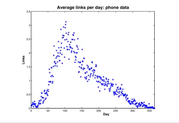
We begin with the “Reality Mining” telecommunication data from [6]. In this case there are 106 nodes and we summarize into 365 days: (A[k])_ij = (A[k])_ji = 1 means that nodes iand j communicated by telephone at least once on dayk. Here max_kρ(A[k]) = 8.2, so the upper limit forais 0.12, and we usea= 0.05.

In Figure 5.1 we show how the average number of links per node varies over time. We see a build up of activity that peaks at around day 100. Figure 5.2 summarizes the network communicability by showing the evolution of||S[k]||, scaled by its maximum, where || · || denotes the Euclidean norm. The upper picture uses b = ∞ (more precisely,e−bΔt= 0 in (3.1)), which corresponds to the static Katz centrality applied at each daily snapshot. We see that this measure closely follows the overall links-per-day structure across time. The middle picture usesb = 0.2, soe−bΔt=e−b = 0.82, allowing us to capture the effect of earlier activity propagating across the network. We see that the running centrality measure presents a much smoother temporal summary and highlights a later period, from around days 140 to 200, as the most influential, with distinct bimodal structure. There is a “lag time” of around 50 days between peaks for the static and running summaries. This lag time was found to depend quite strongly on the parameterb, but the bimodal structure of the running summary was persistent: the lower picture usesb= 0.4, soe−bΔt=e−b= 0.67, and we see that the lag is much shorter. With bincreased to 0.6 the picture becomes very similar to the

b=∞case.

0 50 100 150 200 250 300 350 0

0.5 1

Day

||S

[k]

||

b = ∞

0 50 100 150 200 250 300 350

0 0.5 1

Day

||S

[k]

||

b = 0.2

0 50 100 150 200 250 300 350

0 0.5 1

Day

||S

[k]

||

b = 0.4

Fig. 5.2 Test on “Reality Mining” data. Upper: size of the running dynamic communicability

matrix,S[k], whenb=∞, equivalent to Katz centrality. Middle: b= 0.2. Lower: b= 0.4.

The second experiment uses email data between Enron employees [15], as studied previously, for example, in [10, 21]. We have 151 nodes in the network with interaction summarized over 1138 days. Because email is a one-way form of communication, we use directed links, with (A[k])_ij= 1 if personiemailed personj at least once on day

k. We regardTo:,cc:, andbcc: as equivalent, for simplicity. Figure 5.3 displays the average number of links per node over time. We have maxkρ(A[k]) = 3.93, giving an upper limit of 0.25 fora, and we choosea= 0.2. Our aim is to use current information

{A[0]_{, A}[1]_{, A}[2]_{, . . . , A}[k]_{} to predict the next day’s behavior. We focus on centrality}

and target tomorrow’s Katz-style broadcast and receive centralities, given by

(5.1) (I−aA[k+1])−11 and (I−aA[k+1])−T1,

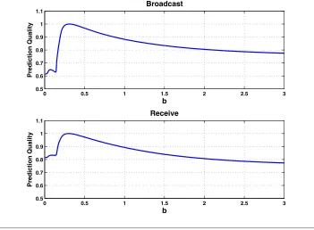
respectively. At each time point k = 0,1, . . . , M −1 we test whether the dynamic broadcast communicabilities assigned to each node by (3.6) match tomorrow’s actual Katz broadcast centralities in (5.1) by computing the Pearson correlation coefficient between the two vectors. We sum the correlation coefficients over all time points (ignoring cases where the adjacency matrix, A[k+1], was empty) to give an overall quantification of how well the dynamic summary predicts future behavior, with a larger value indicating better performance. We also do the same for receive centrality. The upper and lower pictures in Figure 5.4 give the results for broadcast and receive centralities, respectively, as a function of the time-downweighting parameter,

b. These are normalized to have a maximum of 1. Here, b = ∞ corresponds to using only today’s network to predict tomorrow’s andb= 0 corresponds to letting all earlier days have equal influence. We see that the best performance arises with an intermediate case ofb≈0.3, where, for example, walks that started three days ago are

0 200 400 600 800 1000 0

0.1 0.2 0.3 0.4 0.5 0.6 0.7 0.8 0.9 1

Day

Links

Average links per day: email data

Fig. 5.3 Enron email data. Average links per node on each day.

0 0.5 1 1.5 2 2.5 3

0.5 0.6 0.7 0.8 0.9 1 1.1

b

Prediction Quality

Broadcast

0 0.5 1 1.5 2 2.5 3

0.5 0.6 0.7 0.8 0.9 1 1.1

b

Prediction Quality

Receive

Fig. 5.4 Test on Enron email data. Upper: prediction quality for broadcast centrality as a function

of the downweighting parameterb. Lower: receive centrality.

downweighted bye−3b≈0.41 and walks that started two weeks ago are downweighted bye−14b ≈0.015. This test indicates how the choice ofbcan be informed by studying a quantity of interest on real data.

6. Discussion. We believe that the new iteration (3.1) can form the basis of many useful tools aimed at analyzing temporal networks. For example:

• If the iteration is applied in real time, the resulting centrality measures (3.6) can identify the latest “hot” players and those currently on rapid upward or downward trajectories.

• The dynamic summary S[k] can be used to predict likely upcoming links (estimating future bandwidth) or to interfere effectively with the network evolution (suggesting new friends in an online social network or recommending movies in a rental service). Here the static Katz measure, corresponding to

b=∞, has proved successful [17].

• The behavior of S[k] for appropriate time-dependent random graph models, for example, from the class in [9], could provide a baseline against which to calibrate unusual network behavior.

• By applying a clustering method to the running dynamic communicability matrix S[k] at each time point, we could detect sets of nodes that organize into tightly connected communities and then disperse over time. This would give an alternative to the approach in [18].

• The running dynamic broadcast and receive centralities in (3.6) could be used to rank nodes and compare them with known hierarchical structure— for example, job status within a company—in order to see who is punching above their weight.

• In general,S[k]will evolve into a dense matrix, so very-large-scale applications are not feasible. It is therefore of interest to devise fast and low storage algorithms that use approximations ofS[k], along the lines of those developed in the static case [2].

Acknowledgment. The Enron email data was originally collected and prepared by members of the CALO Project (A Cognitive Assistant that Learns and Organizes). We obtained the data from the website http://www.cs.cmu.edu/˜enron/.

REFERENCES

[1] D. S. Bassett, N. F. Wymbs, M. A. Porter, P. J. Mucha, J. M. Carlson, and S. T. Grafton_{,Dynamic reconfiguration of human brain networks during learning, Proc. Nat.}

Acad. Sci. USA, 18 (2011), pp. 7641–7646.

[2] F. Bonchi, P. Esfandiar, D. F. Gleich, C. Greif, and L. V. S. Lakshmanan_{,Fast matrix}

computations for pair-wise and column-wise commute times and Katz scores, Internet Math., 8 (2012), pp. 73–112.

[3] S. Borgatti, K. Carley, and D. Krackhardt_{,On the robustness of centrality measures}

under conditions of imperfect data, Social Networks, 28 (2006), pp. 124–136.

[4] S. Borgatti, A. Mehra, D. Brass, and G. Labianca,Network analysis in the social sciences,

Science, 323 (2009), pp. 892–895.

[5] J. J. Crofts and D. J. Higham_{,Googling the brain: Discovering hierarchical and asymmetric}

network structures, with applications in neuroscience, Internet Math. (Special Issue on Biological Networks), 7 (2011), pp. 1–22.

[6] N. Eagle and A. Pentland_{,Reality mining: Sensing complex social systems, Personal}

Ubiq-uitous Comput., 10 (2006), pp. 255–268.

[7] E. Estrada_{,The Structure of Complex Networks, Oxford University Press, Oxford, 2011.}

[8] E. Estrada, N. Hatano, and M. Benzi_{,The physics of communicability in complex networks,}

Phys. Rep., 514 (2012), pp. 89–119.

[9] P. Grindrod and D. J. Higham_{,Evolving graphs: Dynamical models, inverse problems and}

propagation, Proc. R. Soc. Lond. Ser. A Math. Phys. Eng. Sci., 466 (2010), pp. 753–770. [10] P. Grindrod, D. J. Higham, M. C. Parsons, and E. Estrada_{, Communicability across}

evolving networks, Phys. Rev. E, 83 (2011), 046120.

[11] P. Holme and J. Saram¨aki_{,Temporal networks, Phys. Rep., 519 (2012), pp. 97–125.}

[12] D. Huffaker_{,Dimensions of leadership and social influence in online communities, Human}

Commun. Res., 36 (2010), pp. 593–617.

[13] L. Isella, M. Romano, A. Barrat, C. Cattuto, V. Colizza, W. Van den Broeck, F. Ge-sualdo, E. Pandolfi, L. Rav`a, C. Rizzo, and A. E. Tozzi_{,Close encounters in a}

pedi-atric ward: Measuring face-to-face proximity and mixing patterns with wearable sensors, PLoS ONE, 6 (2011), e17144.

[14] L. Katz, A new index derived from sociometric data analysis, Psychometrika, 18 (1953),

pp. 39–43.

[15] B. Klimt and Y. Yang_{, Introducing the Enron corpus, in First Conference on Email and}

Anti-Spam (CEAS), Mountain View, CA, 2004.

[16] J. Leskovec, L. A. Adamic, and B. A. Huberman_{,The dynamics of viral marketing, in}

Proceedings of the 7th ACM Conference on Electronic Commerce (EC ’06), ACM, New York, 2006, pp. 228–237.

[17] Z. Lu, B. Savas, W. Tang, and I. Dhillon_{,Supervised link prediction using multiple sources,}

in Proceedings of the 10th IEEE International Conference on Data Mining (ICDM), 2010, pp. 923–928.

[18] P. J. Mucha, T. Richardson, K. Macon, M. A. Porter, and J.-P. Onnela_,

Commu-nity structure in time-dependent, multiscale, and multiplex networks, Science, 328 (2010), pp. 876–878.

[19] M. E. J. Newman_{,Networks: An Introduction, Oxford University Press, Oxford, 2010.}

[20] M. Szell, R. Lambiotte, and S. Thurner_{,Multirelational organization of large-scale social}

networks, Proc. Natl. Acad. Sci. USA, 107 (2010), pp. 13636–13641.

[21] J. Tang, M. Musolesi, C. Mascolo, V. Latora, and V. Nicosia_{,Analysing information}

flows and key mediators through temporal centrality metrics, in Proceedings of the 3rd Workshop on Social Network Systems (SNS ’10), ACM, New York, 2010, pp. 1–6. [22] J. Tang, S. Scellato, M. Musolesi, C. Mascolo, and V. Latora_{,Small-world behavior in}

time-varying graphs, Phys. Rev. E, 81 (2010), 05510.

[23] S. Wasserman and K. Faust_{,Social Network Analysis: Methods and Applications, Cambridge}

University Press, Cambridge, UK, 1994.