City, University of London Institutional Repository
Citation: Mansour, M. (2004). Issues in on-line optimisation. (Unpublished Doctoral thesis, City University London)
This is the accepted version of the paper.
This version of the publication may differ from the final published version.
Permanent repository link: http://openaccess.city.ac.uk/8414/ Link to published version:
Copyright and reuse: City Research Online aims to make research outputs of City, University of London available to a wider audience. Copyright and Moral Rights remain with the author(s) and/or copyright holders. URLs from City Research Online may be freely distributed and linked to.
City Research Online: http://openaccess.city.ac.uk/ [email protected]
ISSUES IN ON-LINE OPTIMISATION
By
Moufid Mansour
A THESIS SUBMITTED FOR THE DEGREE OF DOCTOR OF
PHILOSOPHY
CITY UNIVERSITY, LONDON
SCHOOL OF ENGINEERING AND MATHEMATICAL SCIENCES CONTROL ENGINEERING RESEARCH CENTRE
To
My dear mother,
My dear father.
My only brother Mahdi.
My sisters
Karima, Fatiha, Leila, Ouassila, Amal.
My nephews and nieces
Mohamed-amine, Zahra, Sarah, Haroun, Ramzi
The beautiful memory of my grandfather and grandmother.
The beautiful memory of my uncle Tounsi.
The memory of
TABLE OF CONTENTS
TABLE OF CONTENTS 3
LIST OF TABLES 9
LIST OF FIGURES 10
ACKNOWLEDGEMENTS 15
DECLARATION 16
PUBLICATIONS 17
ABSTRACT 18
NOMENCLATURE 19
LIST OF GREEK SYMBOLS 22
LIST OF ABREVIATIONS 23
CHAPTER 1. INTRODUCTION 25
1.1 OPTIMISATION 25
1.2 ON-LINE OPTIMISATION 26
1.2.1 AUTOMATIC DETECTION OF STEADy-STATE 27
1.2.2 DATA RECONCILIATION 28
1.2.3 GROSS ERROR DETECTION 28
1.2.4 PARAMETER ESTIMATION 29
1.2.5 PROCESS OPTIMISATION 29
1.3 OBJECTIVES OF THE THESIS 29
1.4 THESIS SCOPE 30
1.5 THESIS OUTLINE 30
CHAPTER 2. THE ISOPE ALGORITHM 33
2.1 INTRODUCTIOIN 33
2.2 THE ISOPE ALGORITHM AND ITS DEVELOPMENT 35
2.3 FORMULATION OF THE PROBLEM 36
2.4 SPECIAL CASE: QUADRATIC OBJECTIVE WITH LINEAR MODEL
AND CONSTRAINTS 40
2.5 A SIMPLIFIED VERSION OF THE ISOPE ALGORITHM 43
2.6 CONVERGENCE PROPERTIES 44
2.7 SUMMARY 46
CHAPTER 3. CASE STUDY SySTEMS 47
3.1 INTRODUCTION 47
3.2 EXAMPLE 1 48
3.3 EXAMPLE 2: THE TWO CONTINUOUS STIRRED TANK REACTORS
(CSTR'S) 48
3.4 IMPLEMENTATION ISSUES 51
3.5 SUMMARY 53
CHAPTER 4. THECHNIQUES FOR THE ESTIMATION OF THE
DERIVATIVE INFORMATION 54
4.1 INTRODUCTION 54
4.2 FINITE DIFFERENCE APPROXIMATION METHOD (FDAM) 55
4.3 METHOD FOR DUAL CONTROL OPTIMISATION 57
4.4 BROYDON'S METHOD 59
4.5.1 DMI WITH LINEAR MODEL REPRESENTATION 62
4.5.2 DMI WITH A NON-LINEAR MODEL REPRESENTATION 69
4.6 SIMULATION CASE STUDY 72
4.6.1 OPTIMISATION OBJECTIVES AND GOALS 72
4.6.2 RESULTS AND DISCUSSION 76
4.7 SUMMARY 81
CHAPTER 5. A NEURAL NETWORK APPROACH
5.1 INTRODUCTION 82
5.1.1 HISTORY AND DEVELOPMENT OF NEURAL NETWORKS 85
5.2 MULTILAYER AND RECURRENT NETWORKS 86
5.2.1 MULTILAYER FEEDFORWARD NETWORKS 87
5.2.2 RECURRENT NETWORKS 90
5.3 THE BACKPROPAGATION ALGORITHM 92
5.4 THE CONTROL PROBLEM AND THE NEURAL NETWORK SCHEME 96
5.4.1 THE OPTIMISATION PROBLEM AND THE ISOPE ALGORITHM .. 96
5.4.2 THE NEURAL NETWORK SCHEME 97
5.4.3 IDENTIFICATION 98
5.5 SIMULATION CASE STUDIES 100
5.5.1 CASE STUDY 1 100
5.5.2 CASE STUDY 2 105
5.5.2.1 SIMULATION RESULTS 107
5.6 SUMMARY 110
CHAPTER 6. DATA RECONCILIATION AND GROSS ERROR DETECTION 112
6.1 INTRODUCTION 112
6.2 DATA RECONCILIATION 113
6.2.1 TYPES OF ERRORS 114
6.2.2 MEASUREMENT DATA PROCESSING 114
6.2.3 HISTORY 116
6.2.4 BENEFITS 118
6.2.5 RECENT DEVELOPMENTS AND SOFTWARE PACKAGES 118
6.2.6 MATHEMATICAL STRUCTURE OF THE DATA
RECONCILIATION PROBLEM 119
6.2.6.1 NONLINEAR PROGRAMMING (NLP) 121
6.2.6.2 QUADRATIC PROGRAMMING (QP) 121
6.2.6.3 SUCCESSIVE LINEARISATION 122
6.3 GROSS ERROR DETECTION 123
6.3.1 FORMULATION OF THE GLR METHOD FOR GROSS ERROR
DETECTION 124
6.3.2 BIAS ESTIMATION 129
6.4 STRATEGY FOR MULTIPLE GROSS ERROR DETECTION 130
6.4.1 THE SERIAL COMPENSATION STRATEGy 130
6.5 SIMULATION CASE STUDy 133
6.5.1 THE SYSTEM 134
6.5.2 THE SIMULATIONS 134
6.5.3 THE RESULTS 136
6.5.4 DISCUSSION OF THE RESULTS 140
6.6 SUMMARY 140
CHAPTER 7. GROSS ERROR DETECTION AND DATA RECONCILIATION
IN ON-LINE OPTIMISATION 142
7.1 INTRODUCTION 142
7.2 DATA RECONCILIATION 143
7.3 THE ON-LINE OPTIMISATION PROBLEM AND THE ISOPE
ALGORITHM 144
7.4 SIMULATION CASE STUDY 1..+6
7.5 SUMMARY 157
CHAPTER 8. THE METHODOLOGY OF ON-LINE OPTIMISATION 158
8.1 INTRODUCTION 158
8.1.1 METHODOLOGY OF ON-LINE OPTIMISATION 160
8.2 AUTOMATIC DETECTION OF STEADy-STATE 162
8.2.1 APPLICATION 167
8.3 DATA RECONCILIATION 175
8.4 GROSS ERROR DETECTION 177
8.5 COMBINED GROSS ERROR DETECTION AND DATA
RECONCILIATION 183
8.5.1 MEASUREMENT TEST 183
8.5.2 TJOA AND BIEGLER'S CONTAMINATED GAUSSIAN
DISTRIBUTION 187
8.5.3 ROBUST FUNCTION METHOD 190
8.6 PARAMETER ESTIMATION 192
8.7 VARIANCE-COVARIANCE MATRIX ESTIMATION 195
8.8 OPTIMISATION 196
8.8.1 THE ISOPE ALGORITHM 199
8.9 SIMULATION CASE STUDIES 200
8.9.1 RESULTS 202
8.9.2 DISCUSSION OF THE RESULTS 203
8.10 SUMMARY 208
CHAPTER 9. CONCLUSIONS AND RECOMMENDATIONS 209
9.1 CONCLUSIONS 209
9.2 RECOMMENDATIONS FOR FUTURE RESEARCH 215
REFERENCES 217
APPENDIX A 228
APPENDIX B 230
APPENDIX C 232
LIST OF TABLES
Table No. Page
4.1
4.2 4.3
5.1
6.1
7.1
Tuning the identifier parameters
ISOPE algorithm with the different estimation techniques Derivatives Comparison table
Derivatives Comparison table
Bias values and their estimates
ISOPE with neural network scheme when data reconciliation is applied
9
75 75 77
109
137
Figure No.
LIST OF FIGURES
Page
2-1 2-2
The two-step Method The ISOPE algorithm
34 39
3-1 SIMULINK implementation example of the SISO non-linear plant 48 3-2
3-3
The two Continuous Stirred Tank Reactors system
SIMULINK implementation example of the CSTR system
50 53
4-1 The DMI notion aspect 62
4-2 The moving Horizon aspect 63
4-3 FDAM method 78
4-4 Broydon's method 78
4-5 Dual control method 79
4-6 DMI with linear model method 79
4-7 DMI with nonlinear model method 80
4-8 DMI with linear model in noise contaminated case 80
4-9 Objective function graph 81
5-1 A multilayer feedforward neural network with 8 input nodes, 88 3 hidden and 2 output neurons
5-2 Bloc diagram representation of a two layer network 89
5-3 Example plot of the sigmoidal function 89
5-4 Architecture graph of a Recurrent network (Hopfield type) 89 forN = 4 neurons
5-5 Recurrent network with hidden neurons 91
5-6 Bloc diagram representation of a Hopfield network 91
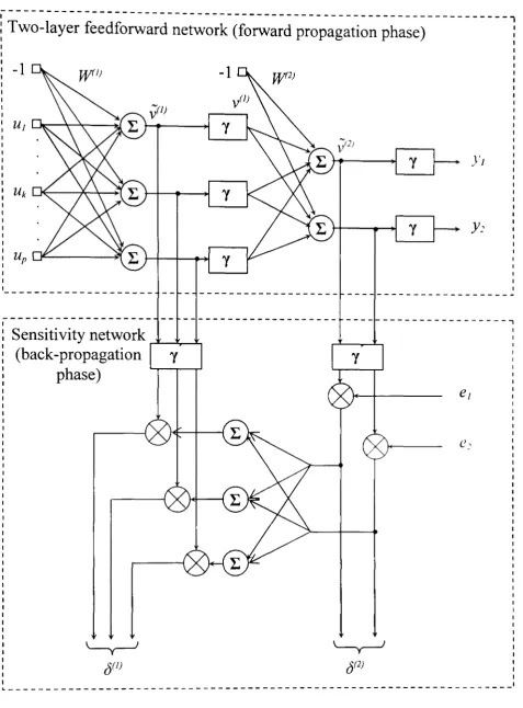
5-7 Architecture of two-layer feedforward network and its associated 93
back-propagation signal error
5-8 Neural Networks scheme used within the ISOPE algorithm 98 5-9 Flow chart diagram representation of the neural network scheme 99 5-10 Outputs of the real plant and the neural net. identification model 102 5-11 Outputs of the plant and the neural net. identification model 102
when input changes
/\
5-12 Plots ofy
=
j(u)and y=
N[ u] for real process and identification 102model
5-13 Outputs of the real plant and the RBF network identification model 104 5-14 Outputs of the plant and the RBF network identification model 104
when input changes /\
5-15 Plots ofy
=
j(u) and y=
N[u] for real process and the RBF 104Network identification model
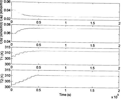
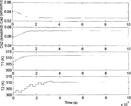
5-16 Set-points changes and outputs trajectories for the FDAM method 109 5-17 Set-points changes and outputs trajectories for the neural network 110
scheme
6-1 Three steps for processing measurement data 115
(Liebman et al., 1992).
6-2 Variable classification 116
6-3 Bloc diagram representation of the GLR algorithm 128 6-4 Reconciliation when measurement were subject to noise but 138
without bias
6-5 Reconciliation when only one measurement ChI was biased 138
6-6 Reconciliation when only one measurement Ch2 was biased 139 6-7 Reconciliation when both measurements ChI and Ch2 were biased 139
7-1 The two-step Method 1..+5
7-'2 Schematic representation of the SDR and GED scheme within the 1..+6
ISOPE algorithm
7-3 Bloc diagram representation of the application of the DR and GED 149 scheme within the ISOPE algorithm
7-4 Real process output and noisy measurements trajectories, case 152 when optimisation was applied when both measurements were
affected by noise without data reconciliation
7-5 Set-points trajectories, case when optimisation was applied 152 when both measurements were affected by noise without data
reconciliation
7-6 Real process output and noisy measurements trajectories, case 153 when optimisation was applied when both measurements are
affected by noise with data reconciliation
7-7 Set-points trajectories, case when optimisation was applied when 153 both measurements are affected by noise with data reconciliation
7-8 Real process output and noisy measurements trajectories, case 154 when optimisation was applied when ChI was biased with data
reconciliation
7-9 Set-points trajectories, case when optimisation was applied when 154
ChI was biased with data reconciliation
7-10 Real process output and noisy measurements trajectories, case 155 when optimisation was applied when C h2 was biased with data
reconciliation
7-11 Set-points trajectories, case when optimisation was applied when 155
Ch2 was biased with data reconciliation
7-12 Real process output and noisy measurements trajectories, case 156 when optimisation was applied when ChI and C h2 were biased
with data reconciliation
7-13 Set-points trajectories, case when optimisation was applied when 156
ChI and C
h2were biased with data reconciliation
8-1 8-2
Schematic representation of on-line optimisation No auto-correlation in variable (tal
12
8-3 No cross-correlation between ChI and C h2 170
8-4 R-value and SS trajectories for Cal 171
8-5 R-value and SS trajectories for ChI 171
8-6 R-value and SS trajectories for C a 2 172
8-7 R-value and SS trajectories for C h2 1'""'1
/-8-8 Cal and SS trajectories 173
8-9 C a2and SS trajectories 173
8-10 ChI and SS trajectories 174
8-11 C h2and SS trajectories 174
8-12 Output vector and overall SS trajectories 175
8-13 Types of gross errors (Narasimhan and Jordache, 2000) 178
8-14 On-line Optimisation Procedure 201
8-15 Real process output and noisy measurement trajectories, 204 case when the methodology was not applied with both
measurements affected by noise only
8-16 Set-point trajectories, case when the methodology was not 204 applied with both measurements affected by noise only
8-17 Real process output and noisy measurement trajectories, 205 case when the methodology was not applied with both
measurements affected by noise and Ch:l is biased
8-18 Set-point trajectories, case when the methodology was not 205 applied with both measurements affected by noise and C h2
is biased
8-19 Real process output, noisy and reconciled measurement 206 trajectories, case when the methodology was applied with
('h2 biased
8-20 Set-point trajectories, case when the methodology was 206 applied with Ch:l biased
8-21 Real process output, noisy and reconciled measurement 207 trajectories, case when the methodology was applied with
Ch2 biased after eliminating wasted time
8-22 Set-point trajectories, case when the methodology was applied with Ch2 biased after eliminating wasted time
14
ACKNOWLEDGEMENTS
I would like to express my sincere thanks and gratitude to my supervisor, Doctor Joe E. Ellis for his guidance, encouragement, help and patience throughout the course of this research.
I would also like to thank Dr. V. M Becerra who provided many useful suggestions and support which enhanced the quality of this work.
I wish also to add a special note of thanks to the Algerian government for having funded my studies here at City University.
I would like to thank my mother for her patience, support, encouragement and prayers throughout and my father for his valuable guidance and confidence.
My thanks are due to Kamal, Mahdi, Halim, Chris, Yasser and Shagufta for their encouragement.
Last, but by no means least, I would like to express my thanks to my fellow research colleagues in the Control Engineering Research Centre for their help and encouragement. Thanks to Ziad, Daniel, Stavros, Costas, Ali, Ermina, Tanya, Dimitrios, Dia, Ram and Gabriel. My thanks also to Joan Rivellini and Linda Carr in the Electrical Engineering office for their tireless and caring attitude to help at all times.
DECLARATION
The author grants powers of discretion to the University Librarian to allow this thesis to be copied in whole or part without further reference to him. This permission covers only single copies made for study purposes, subject to normal conditions of acknowledgement.
PUBLICATIONS
The following is a list of publications based on the work described in this thesis:
1. Comparison of methods for estimating real process derivatives in on-line optimisation, Mansour M., Ellis J.E., Applied Mathematical Modelling, Vol. 27,pp.275-291,2003.
2. Issues in On-line Optimisation, Mansour M., Ellis lE., Technical Report no. 174, CERC, City University, London, UK, April 2000.
The following papers based on the work described in this thesis, have been submitted for publication:
1. Process Optimisation with the aid of Artificial Neural Networks, Mansour M.,
Ellis J.E., Applied Artificial Intelligence.
2. Methodology of On-line Optimisation Applied to a Chemical Reactor,
Mansour M., Ellis lE., Applied Mathematical Modelling.
3. Data Reconciliation and Gross Error Detection in On-line Optimisation,
Mansour M., Ellis lE., International Journal ofControl.
ABSTRACT
In general, on-line optimisation can be defined as the on-line process of finding the optimum set-points of the system. Several areas might be concerned in this procedure. This thesis evaluates algorithms for on-line Optimisation. Techniques for steady-state detection, static data reconciliation, gross error detection and steady-state optimisation are presented and implemented separately and within an on-line optimisation methodology.
It has been acknowledged for some time now that the estimation of derivative information is probably the major drawback of the steady-state optimisation technique considered here: the ISOPE algorithm. This thesis investigates the requirements of these derivatives, methods proposed to estimate them, and presents some attempts to overcome some related problems. Also a modified version of the dynamic model identification method that uses a nonlinear model representation is proposed, and compared under simulation with other available techniques. In the same context, an alternative method based on Artificial Neural Networks to estimate the derivatives is also implemented and tested.
Often, rigorous steady-state detection is crucial for process performance assessment, simulation, optimisation and control. In general, at steady-state data is collected for safe, beneficial and rational management of processes. A method for automatic detection of steady-state in multivariable processes is implemented and tested. The technique is applied on a dynamic model of a chemical reactor.
The presence of errors in process measurements can invalidate the potential gains obtained from advanced optimisation and control techniques. Data reconciliation and gross error detection methods are used to reduce the inaccuracies of these measurements. The implementation and application of static data reconciliation and gross error detection techniques in this thesis show a noticeable improvement in the operation of the system, and general control system performance.
The various algorithms mentioned above are successfully implemented and tested under simulation. It is illustrated that in some cases, it is possible to use steady-state detection in conjunction with data reconciliation, gross error detection, parameter estimation and optimisation, to form an on-line optimisation methodology. The methodology was tested on a dynamic model of a chemical reactor.
Symbol
a
d~,i
e
f
g H
1
K
171'
NOMENCLATURE
Definition
Gain Matrix
Polynomial matrix
Vector of measurement adjustments Polynomial matrix
Vector of bias parameters Bias estimate
Broydon's update matrix Weighting matrix
Weighting matrix
Minimum pure time delay
Filtered square difference of successive data Weighting vector
Residual ofith process measurement Weighting vector
Directional derivatives
Mapping of output dependent inequality constraints Model input-output mapping
Real process input-output mapping Identity matrix
Relaxation gain matrix Filter factors
Length of data window Model updating period
Size of measured outputs vector
Pu P(.) P period Q -I q R r
SS
T uv
vVmin, Vmax
1'(1)
x
r.,
, ,/l'
y
Size of manipulated variables vector
Vector of price coefficients for manipulated variables
Vector of price coefficients for measured variables
Fixed and updated parameter vectors
Probability distribution function
Integer ratio between data window length and model updating
Objective function
Backward shift operator
Auxiliary matrix
Critical value of R-statistic
Convexification factor
Steady-state identification variable
Sampling time
Vector of decision variables
Controls lower and upper bounds
Desired value for the decision variable vector
Element i of the external input vector
Covariance matrix
Vector of manipulated variables
Lower and upper bounds for the vector of manipulated variables
Vector of net internal activity levels of neurons in layer I
Vector of function signals of neurons in layerI
State vector
Process measured variable at time i.
Filtered value ofX at time i.
Vector of model outputs
Vector of measured variables
"-Y
Ymin' Y max
Ym
z'
w
Predicted future outputs
Bounds on measured variables
Vector of measured process variables Reference value for the measured variable Elementj of the network output vector Vector of true process variables
Unit delay
Synaptic weight vector of a neuron in layerI
Set of relaxation variables
a
e
rp
P
17
S
s.
.Ir
r
A
List of Greek Symbols
Vector of free parameters
Level of significance of variable i Increment operator
Vector of random measurement errors Vector of gross errors
Standardised measurement error Vector of random errors
Terminal state weighting matrix Average squared error
Lagrange multiplier Forgetting factor
Least squares parameter matrix Least squares regression vector Penalty factor
Learning-rate parameter Perturbation signal
Maximum allowed value
Minimal and maximal singular values
Vector of local gradients of neurons in layer I
Auxiliary matrix Activation function
Abbreviation ADALINE AI AISOPE ALMISOPE ANN ARMA ARMAX BIBO CSTR DCS DISOPE DMI DR EVM FDAM GED GLR ISOPE LMS M-file MADALINE MIMO NLP ODE PRBS
List of Abbreviations
Description
ADAptive LINear Element Artificial Intelligence
Augmented ISOPE
Approximate Linear Model ISOPE Artificial Neural Networks
Auto Regressive Moving Average
Auto Regressive Moving Average with Exogeneous input Bounded Input Bounded Output
Continuous Stirred Tank Reactors Distributed Control System
Dynamic Integrated System Optimisation and Parameter Estimation
Dynamic Model Identification Method Data Reconciliation
Errors in Variables Measured
Finite Difference Approximation Method Gross Error Detection
Generalized Likelihood Ratio
Integrated System Optimisation and Parameter Estimation Least Mean Squares
Matlab file
Multiple ADALINE Multi Input Multi Output Nonlinear Programming
QP SDR SISO SQP WLS
Quadratic Programming
Steady-state Data Reconciliation Single Input Single Output
Sequential Quadratic Programming Weighted Least-Squares
CHAPTERl
INTRODUCTION
On-line Optimisation techniques have been in existence for quite some
time and yet few industrial applications have been implemented to date. This may
stem from the general attitude in many manufacturing environments, where
advanced technologies not fully understood are rejected. In addition there are
tendencies to approach control problems from the traditional side, especially
if
the solution works "well enough ".
1.1 OPTIMISATION
Optimisation, in the context of this work, may be thought of as the science of determining the 'best' solutions to certain mathematically defined problems, which are often models of physical reality. It involves the study of optimality criteria for problems, the determination of algorithmic methods of solution, the study of the structure of such methods, and computer experimentation with methods both under trial conditions and on real life problems (Fletcher, 1980).
The concept of optimisation is now well rooted as a principle underlying the analysis of many complex decision or allocation problems. It offers a certain degree of philosophical elegance that is hard to dispute, and it often offers an indispensable degree of operational simplicity.
In a mathematical cense, Optimisation may be concerned with finding the minimum (or maximum) of an objective function, where there may exist
restrictions or constraints as to what are permissible values of the independent variables.
Generally, it not possible to fully represent all the complexities of variable interactions, constraints, and appropriate objectives when faced with a complex decision problem, a particular optimisation formulation should be regarded only as an approximation like all quantitative techniques of analysis.
1.2 ON-LINE OPTIMISATION
On-line optimisation is an approach for trying to maintain a plant at its optimum operating conditions by determining the required set-points of the plant. In the majority of cases, the set-points will be made available to the plant's Distributed Control System (DCS), although they could be used by a stand-alone computer system. In most industrial processes, the optimal operating point is continually shifting in response to changing market demands for products, fluctuating costs of raw materials, products and utilities, and changing equipment efficiencies and capacities. In addition, ambient conditions, variations in feed quality and availability, and changes in equipment configuration are additional constraints that can alter the location of the optimal operation point. The time frame over which these various changes can occur ranges from minutes to months. The competitive economic environment requires timely response to these changing factors. This means that the optimisation must be carried out on-line to have the plant operate continually under the best conditions.
On-line optimisation takes advantage of the fact that plants generally operate at steady-state and have transient periods that are relatively short compared to steady-state operations. Therefore, in on-line optimisation, steady-state models are usually able to be used to describe these plants and their behaviour. The basic methodology of on-line optimisation adopted in this thesis is to automatically detect steady-state from the data samples collected from the process itself, reconcile them to remove any random and! or gross errors, to update parameters in the plant model in order to obtain plant-model matching. Then the current plant
and its model are used to conduct optimisation and to generate a set of optimum set-points. This procedure is able to be run continuously to cope with the possibility of internal conditions (plant parameters and plant configuration) and/or external conditions (economic parameters) changing.
Besides determining the optimum operating condition of the process from the solution of the on-line optimisation problem, a number of other benefits are also apparent. The detail operation information generated from on-line optimisation provides a better understanding of the processes; this can be used to de-bottleneck the process and to improve operating difficulties. Also, abnormal measurement information obtained from gross error detection can help instrument and process engineers to trouble shoot the plant instrument errors. Parameter estimation is very useful for process engineers to evaluate the equipment conditions and to identify the decreasing efficiencies and problem sources. Furthermore, the detailed process simulation from on-line optimisation can be used for process monitoring and serves as a training tool for new operators to obtain first hand operating experience.
There are a number of areas which are central to the work and these are briefly introduced in Sections 1.2.1-1.2.5
1.2.1. Automatic Detection of Steady-State
Process owners analyse processes when they are at steady-state, for this reason, and for the reason that static data reconciliation and process optimisation are steady-state procedures, it is important that the process has to be at steady-state before applying the data reconciliation and optimisation procedures. Identification of the steady-state can prove to be difficult because process variables may be noisy and measurements do not settle. So. steady-state identification requires statistical tests to compensate for the noisy data.
1.2.2. Data Reconciliation
Measured process data inherently contains inaccurate information. This is due to the fact that measurements are obtained using imperfect techniques. Using this inaccurate information to estimate process variables and control the process. results in the state of the system to be misrepresented and the control performance to be poor, leading to sub-optimum and even unsafe process operation. The objective of data reconciliation is to correct measured data variables so they obey natural laws, such as energy and mass balances. Unfortunately, in the presence of biases, all the adjustments can be greatly affected by these types of gross error, and would in general not be reliable indicators of the state of the process.
1.2.3. Gross Error Detection
Raw process data is subject to two types of errors: random errors and gross errors. Random errors are dealt with using data reconciliation techniques, while gross errors need a different type of techniques, namely, gross error detection techniques. Ideally, the aim of a gross error detection technique is to:
1 Detect the existence of the gross error 2 Identify its location
3 Identify its type 4 Determine its size
After the gross errors are identified, two responses are possible and/or desired (Bagajewicz, 2003):
Eliminate the measurement with the bias, or
J Correct the model such as the case of a leak and run the reconciliation again.
1.2.4. Parameter Estimation
Mismatch between models and plants can be due to a number of factors such as: uncertain parameters, unknown state variables, unmeasured disturbances, error in the model structure, and measurement noise. Proper adaptation schemes. where the model parameters are updated on the basis of recent measurements. need to be incorporated into the model-based optimisation control approach to minimise the plant-model mismatch. There exist several approaches to cope with this problem, where all are adaptive in nature but differ in their adaptation schemes.
1.2.5. Process Optimisation
Although there are many different available optimisation techniques, they can be classified into two general categories: direct search and model-based optimisation methods (Garcia and Morari, 1981).
As an on-line optimisation procedure, the Integrated System Optimisation and Parameter Estimation (ISOPE) algorithm (or modified two step in some literature) developed by Roberts in 1979, has some special features which can either be considered as direct or indirect. It is based on a number of features including derivatives calculation, originally estimated by using real process measurements, to update a model used in the model-based optimisation, thus reaching the real optimum of the process in spite of plant-model mismatch. Estimation of the derivatives by means of measurement, which increases geometrically with problem dimensionality, is a major problem of the ISOPE technique.
1.3 OBJECTIVES OF THE THESIS
algorithms for process derivatives estimation, conducting and implementing
steady-state detection, data reconciliation, gross error detection, parameter
estimation and optimisation.
Any improvement in this area should help give more understanding of the way
on-line optimisation has to be implemented, and hence lead to more benefits of
on-line optimisation.
1.4 THESIS SCOPE
This thesis is concerned with certain on-line optimisation structures and the
general ISOPE algorithm which integrates an optimisation scheme together with
parameter estimation. Examples of situations using this structure are presented
within this thesis, and these examples should help to indicate how practical
problems can be treated and structured in this form. The thesis is also concerned
with the analysis and comparison of algorithms and techniques for solving both
general on-line optimisation problems and some related sub-problems. Problems
of steady-state detection, data reconciliation, gross error detection and parameter
estimation are also discussed and treated.
1.5 THESIS OUTLINE
This thesis is structured as follows:
Chapter 2 introduces the well known Integrated System Optimisation and
Parameter Estimation (ISOPE) algorithm developed by Roberts (1979). The
method was developed to overcome the problems of measurements and noise in
the direct optimisation approach, and plant-model differences in the indirect one.
A brief history is given together with the advantages and disadvantages that the
method presents. One major drawback that poses a practical limitation and which
wi II be the basis of some research in the following chapters is the need for real
process output derivatives with respect to the set-points to be computed at each
iteration of the algorithm.
Chapter 3 presents simulation case study systems. Two systems which will be used throughout the thesis for simulation purposes in order to assess and compare the performance and effectiveness of some of the techniques developed and presented in this thesis.
In chapter 4, a comparison study between some of the established methods for real process output derivatives with respect to set-points when used within the ISOPE algorithm and a new method based on a nonlinear dynamic model is made. These methods try to overcome the limitation caused to the ISOPE algorithm, by the need to perturb the system to obtain these derivatives. The methods are implemented under simulation on one of the two case study systems presented in chapter 3, which is the two Continuous Stirred Tank Reactors (CSTR) system. Results of the simulations are then presented and compared
Chapter 5 presents a method for estimating real process derivatives with respect to set-points. This method is based on Artificial Neural Networks (ANN). At first, a brief history is given on ANN's, together with the main philosophy behind the creation of ANN's. The neural network scheme is then presented and tested under simulation on the two systems presented in chapter 3. Results are compared with those obtained using a method described in chapter 4.
Chapter 6 introduces the area of data reconciliation and gross error detection for the use to correct data measurements by removing both random and gross errors from the data set. After a review of previous work, data classification and a description of the problems that both random and gross errors present on on-line optimisation and a full description of data reconciliation and gross error detection techniques is given. The performance of these techniques is demonstrated in a simulation case study. The case study uses the CSTR system described in chapter
Chapter 7 incorporates the techniques implemented in chapter 7 for the static data reconciliation and gross error detection for the elimination of random noise and biases within the ISOPE algorithm. Again, simulations are carried out using the CSTR system. Results of these simulations are discussed and compared to the case when data reconciliation or gross error detection is not implemented.
Chapter 8 presents the on-line optimisation methodology as adopted in our work. and gives a brief description on how each step of the methodology is carried out. Methods for steady-state detection, data reconciliation, gross error detection. parameter estimation and process optimisation are reviewed. Difficulties and drawbacks of each method are discussed and compared to other methods in the literature. Simulation studies were conducted to test some of the key methods on the two Continuous Stirred Tank Reactors (CSTR) system. Finally, the whole methodology was implemented under simulation on the CSTR system. The implemented methodology procedure includes a steady-state detection module connected to a gross error detection module, which in itself connects to a static data reconciliation module. This latter is directly linked to the ISOPE algorithm module for optimisation of the two CSTR system.
The thesis concludes with a number of suggestions for further research related to the work carried out in this thesis.
1.6 SUMMARY
An introduction to the broad area of optimisation was given in this chapter. Specifically, on-line optimisation, which here is considered to be a multi-step procedure consisting of steady-state detection, data reconciliation, gross error detection, parameter estimation and the actual optimisation procedure. One particular method for system optimisation and parameter estimation (lSOPE) was presented. The scope and a short outline of the thesis were also given.
In the next chapter, the ISOPE algorithm is presented in more detail.
' ' l
-'-CHAPTER 2
THE ISOPE ALGORITHM
2.1 INTRODUCTION
The On-line optimisation problem, which consists of the determination of
controls, or set-points, of a system controller, can be divided into two major
categories: the direct and indirect approaches. The direct approach uses
measurements taken directly from the real physical system and applies one of the
basic optimisation techniques to optimise the process performance objective
function. However, in practice this can give rise to some difficulties such as
having to contend with measurement noise and having to allow the process to
settle sufficiently before measurements are taken.
In the indirect or model-based approach, the optimisation is performed on a
mathematical model of the plant instead of the real system itself. When found, the
results are then applied to the real system. The use of model-based approaches has
several advantages. The measurements contaminated by noise and other process
disturbances are largely avoided. Also, there may not be a need to allow the
system to settle before taking measurements or to have available all measurements
of process variables which appear in the performance index (Ellis et aI., 1988).
Again, this is unlikely to produce the process optimum, as it is inevitable that
model-reality differences exist at least to some extent, in terms of structure and
parameter.
To overcome the problems of measurements and noise in the direct approach. and
model-reality differences in the indirect one, the ISOPE (Integrated System
Optimisation and Parameter Estimation) algorithm was introduced (Roberts.
is to replace the model-based optimisation problem, after an analysis of first-order
optimality conditions (Appendix A) by an equivalent problem which is ultimately
decomposed into a parameter estimation problem and a modified model-based
optimisation problem (Roberts et al., 1988). In this method, information gained
from the real process is used to correct the errors occurring in the model. Hence.
reaching the optimum of the real process in spite of model-reality differences.
All ISOPE algorithms designed to date are derived from the basic and well-known
two-step technique, which consists of two major steps. The first step solves. with
the aid of process measurement, a simple model parameter estimation procedure.
The updated model is then used in the optimisation problem. The second step
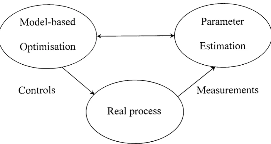
obtains the process controls via an optimisation routine (Figure 2-1). The major
drawback of the two-step method is that it assumes a complete match between the
output derivatives with respect to set-points of the real system and its model. This
is highly unlikely to happen in reality where the degree of non-linearity is very
high and the environments are varying. This problem was addressed by the ISOPE
(sometimes referred to as the modified two-step) method, by introducing a new
modifier variable. This modifier takes into account differences between the real
process and model-based output derivatives with respect to the set-points, which
ensures satisfaction of the system optimality conditions.
Parameter
Estimation
Real process
Optimisation
Model-based
Controls
Figure (2-1): The two-step Method.
[image:35.713.136.598.633.878.2]2.2 THE ISOPE ALGORITHM AND ITS DEVELOPMENT
The ISOPE algorithm as initially proposed by Roberts (1979), deals only with unconstrained problems. It was only until 1986 that Brdys et al. (1986) and then later Lin et al. (1988) extended it to include problems with output independent and output dependent inequality constraints. Nevertheless, the algorithm was used successfully in a large variety of cases before that. Indeed, Ellis and Roberts (1981) used the algorithm for on-line optimisation of a chemical reactor. The results were promising, and opened the door for other researchers to investigate the method more deeply. The performances of the algorithm, particularly the stability and convergence properties as well as the effect of real process measurement errors were investigated by Roberts and Williams (1981). Also, a convergence analysis was conducted by Brdys and Roberts (1987). Ellis et al (1988) conducted a comparison study where three methods were applied to a fuel gas mixer process. The methods compared were the Conjugate direction method, a rationalised form of the ISOPE algorithm and an Approximate Linear Model ISOPE (ALMISOPE) method. It was concluded that in some specific cases, the ALMISOPE is more efficient than the other two methods. An algorithm with dual control effect for which the generated control signal satisfies the main control goal as well as providing sufficient information for future identification action was proposed by Brdys and Tatjewski (1994). Roberts (1992) introduced DISOPE, a dynamic extension of the ISOPE algorithm used for solving nonlinear discrete time optimal control problems. Data reconciliation techniques were also used within the ISOPE algorithm to improve static optimisation schemes where data was contaminated by noise and systematic bias (Abu-el-Zeet, 2000). And lately, a comparison study including the most popular techniques for estimating process derivatives needed by the ISOPE algorithm, was conducted by Mansour and Ellis (2003). In the study, it was shown that the optimum operating point is reached with all the different estimating techniques used, but with a difference in speed of convergence; the Dynamic Model Identification technique being superior. Further work was carried out on the ISOPE algorithm, including: Abdullah (1988) for the
Augmented ISOPE (AISOPE) and Becerra et al (1998) in the area of predictive control. A review of the ISOPE algorithm can be seen in Roberts (1995).
2.3 FORMULATION OF THE PROBLEM
Consider the general steady-state optimisation problem of finding the optimum set-points of a system, which the behaviour obeys to the following relationships:
Vmin <v<vmax
(2.1)
(2.2)
(2.3)
where y* is an ny vector of measured outputs, v is an nil vector of manipulated
variables, H* represents the real process input-output mapping and g is a mapping of output dependent inequality constraints.
The performance of the system is measured with the objective function Q, which is assumed to be continuous, and differentiable.
The system optimisation problem is then considered to be:
Subject to:
Min Q(v,y*)
y*
=
H*(v)\' . <"mill ~ "max
~6
(2.4)
(2.5)
(2.6)
In general, the above system optimisation problem is converted into a
model-based optimisation problem where the following model of the real system is used:
y
=
H(u,a) (2.8)where y is a vector of model outputs, u is a vector of decision variables: H is the
model used to approximate the real process mapping and a is a vector of free
parameters.
After analysis of the 1st order necessary optimality conditions (Appendix A), the
problem (2.4) to (2.7) becomes:
subject to:
min Q(u,y)
y
=
H(u,a)H* (v)
=
H(u,a)v=u
g(y) < 0
(2.9)
(2.10)
(2.11 )
(2.12)
(2.13)
(2.14)
The free parameters a are chosen so that the model and real process outputs match
at the current operating point, the model is then said to be point parametric (Ellis
et al., 1988).
The above equations, after applying the necessary optimality conditions, yield the
following model-based procedure:
subject to:
where
min Q(H(u,a),u)-AU+t pwTw+tr
II
u-v 112u,w
g(H*(v))
+
M(u - v)+
w~ 0-Umin ~ U < U max
-Umin
=
maX(Umin ,v - 5)
-U max = min(umax ,v
+
5)(2.15)
(2.16)
(2.17)
(2.18)
(2.19)
5j is the maximum allowed value of IUj - vj
I,
j=
1,. .. ,nu' M is given by:(2.20)
A is computed from:
and a can be obtained from:
y* - H(v,a)
=
0(2.21 )
(2.22)
Equation (2.16) is equivalent to (2.13), and A is a Lagrange multiplier, usually
referred to as a modifier.
11'is a set of relaxation variables and p is a penalty factor. The term
+
r II U - \' 112 isused only for highly non-convex objective functions and is seen to improve the
convergence of the algorithm (r ~ 0) (Becerra and Roberts, 2000).
The above problem is then treated as a general nonlinear programming problem.
When found, the solution of the problem (Roberts, 1979) is then treated within a
relaxation scheme to give in an iterative manner the next control (see procedure in
section 2.5) as follows:
(2.23)
Where KE [0,1) is a relaxation gain matrix, and governs the actual changes made
to the real process inputs from one iteration to another. Its purpose is to ensure
that excessive alterations are not made.
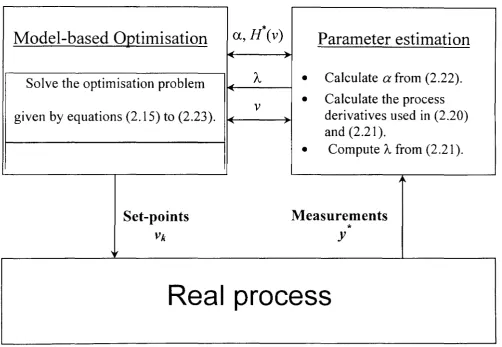
The basic scheme of the algorithm can be seen in Figure (2-2).
*
Model-based Optimisation
o, H (v)Parameter estimation
... ,
A Calculate a from (2.22). Solve the optimisation problem ,
•
•
Calculate the process vgiven by equations (2.15) to (2.23). . J derivatives used in (2.20)
and (2.21).
•
Compute A from (2.21).)
Set-points Measurements
*
Vk Y
'If
Real process
Figure (2-2): The ISOPE algorithm.
From the previous relations (2.20) and (2.21), it can be seen that real process
derivatives are needed in order to compute the modifier A. Various techniques
[image:40.717.110.613.454.801.2]exist and have been developed and applied to date to estimate these derivatives.
Finite Differences Technique using perturbation, based on measurements, was
originally suggested with the algorithm by Roberts (1979). Although simple to
apply, the technique proved to be inefficient in the case of large, slow and
randomly noisy processes. The dynamic model identification method introduced
by Zhang and Roberts (1988). The major advantage the technique brought was the
reduction of the amount of time taken to estimate the derivatives. However. it
encountered some difficulties such as: the huge amount of data needed and the
poor inaccurate model it gives at the beginning of the identification.
Broydon's approximation method, based on the well-known Broydon's family of
formulas, mainly oriented to the approximation of derivatives was also used and
implemented. These techniques are studied in detail in Chapter 4, where an
assessment of their efficiency is made through a simulation of a Continued Stirred
two Tank reactor (CSTR) system. Other methods have been developed with the
aim of totally eliminating the need for the derivative information from within the
ISOPE algorithm. However, these techniques have not proven to be highly
successful, and therefore have not been included in this work.
2.4 SPECIAL
CASE:
QUADRATIC
OBJECTIVE
WITH
LINEAR MODEL AND CONSTRAINTS
Although the structure of most dynamical systems is of non-linear form, it is often
possible to obtain a good linear approximation to the behaviour of the system
around a suitable operating point. Thus, many systems can be described by the
following linear representation:
y=H(u,a)=Au+a
g(y)=Gy-h~O
40
(2.24)
whereA is an (ny xnu ) matrix. And g is the output inequality constraints. In the special case where the objective function
Q
is quadratic of the form:(2.26)
where C and D are symmetric positive definite weighting matrices. e and
f
weighting vectors, Yd and ud are the desired steady-state output and set-pointvectors respectively.
The physical interpretation of such a performance index, is that we desire to maintain the output vector Y close to a target vector value Yd without using
excessive control effort, by keeping U near a given vector value uti. The weighting matrices C and D (Singh and Titli, 1978) enable us to define the relative importance of keeping the output near the desired target, the expenditure of control effort and the need to ensure that at the final time, the output vector will be very close to the desired target (convergence).
The reasons behind using linear models with quadratic performance indices is to be able to use Quadratic Programming to solve the general non-linear problem of finding the optimum point of a given non-linear system (which can prove to be very difficult and time consuming) by converting it into a simplified quadratic problem. One of the principal properties of quadratic programming problems is that the constraints are linear, so they are convex, and in the case of a convex objective function (which can happen if the weighting matrix is positive definite or positive semidefinite). there is a unique solution to the problem which is the global optimum. Quadratic programming arises in many applications and it forms a basis of some specific algorithms and techniques. As it is usually solved using calculus, many problems which are highly non-linear are converted into quadratic formulation. A quadratic program is greatly simplified, and can be solved in closed form if it contains equality constraints only.
In this case the parameter a will be calculated by:
•
a
=
y - Au (2.27)And Acan be found by combining equation (2.21) with (2.24) and (2.26) to be:
(2.28)
In this case the modifier A is found using the above formulation with the help of
process information such as measurement (i.e.: matrix A obtained using
measurements) and optimiser parameters such as D, C, and e.
The optimisation problem therefore IS reduced to the following quadratic
programming problem:
Subject to:
. I TS T
mln2"x x+q x
x
-Gx<h
(2.29)
(2.30)
xm i n < X < xm ax (2.31 )
where:
x=[:]
(2.32)s
=
[ATCA +D+
rIll IOnvx,]°
IXIIr IpI,42
(2.33)
II
=
[b - Gy· - GAv]The above optimisation problem is solved using quadratic programming.
(2.35)
(2.36)
2.5 A SIMPLIFIED VERSION OF THE ISOPE ALGORITHM
A practical version of the ISOPE algorithm presented in this chapter and developed by Becerra and Roberts (2000) is given below. It is worthwhile noting that the convergence of the algorithm for which a summary is given in section 2.6, depends upon several factors. The accuracy of the derivative estimation is one of these factors. The procedure is (Becerra and Roberts, 2000):
Data: C,D,e,j'Yd' ud ' G, h, r, p.K, vk and means for measuringy. and computing Ak • Put k =
a
and go to step l .1. Apply the current input vk to the plant, wait for a steady-state to be reached •
and measure the process outputYk .
2. Update the gain matrix Ak by using one of the available estimation methods presented in chapter 4.
3. Compute ak using (2.27) and Ak using (2.28).
4. Solve the optimisation problem given by equations (2.29) to (2.36) using
quadratic programming to obtain the next input candidateUk +1•
5. Compute the next process input by using (2.23).
6. Set k
=
k+1, check for convergence and go to step 1.These steps are repeated until convergence is reached. Convergence occurs when
no further improvement is observed. In other words, when the new control is no
longer a better candidate than the previous one. Theoretically, convergence is
checked in step 6 by testing the equalityvk+ )
=
Vk• Practically, the previous
equalityvk+)
=
V k is replaced by the following inequality:II
Vk+1- Vk
11<
e . Wheree > 0 is a desired accuracy threshold.2.6 CONVERGENCE PROPERTIES
The convergence and optimality properties of the ISOPE algorithm for on-line
determination of the optimum steady-state operating point of a given process was
investigated in detail by Brdys and Roberts (1987). The conclusion was that,
under mild assumptions, a suitable gain matrix K exists such that every point
generated by the iterative procedure (equation (2.23)) is feasible. In fact, in order
to assure feasibility during iterations for a general constrained case, the gain
matrix K must be of the form:
K=kI
Where k is a positive scalar, and I is the identity matrix.
This involves all individual gains k, to have the same identical numerical values,
unlike in the unconstrained case. where the gain matrix K is allowed to have
diIfcrent individual diagonal elements. However, the scalar parameter k in the constrained case. is allowed to change from one iteration to another
Under such conditions, the process performance index is improved at each
iteration and each cluster point of the sequence generated by the algorithm
satisfies first-order necessary conditions for optimality. Furthermore. everv
optimal point belongs to the solution set of the algorithm.
Although, in order to guarantee convergence, the composition of the performance
index and the process mathematical model should be uniformly convex functional
on the set of admissible controls, the real process input-output mapping may be
non-linear such that its composition with the performance index is not required to
be convex. Hence, the algorithm is applicable to a broad class of real problems
(Brdys and Roberts, 1987).
Also, it was found (Kambhampati, 1988) that:
1. The derivative differences given by [[8H· (J-L)]1' _ [8H (J-L)]7' ]
8J-L JI=1- 8J-L
JI=1-constitute the model-reality differences.
2. The modifier Acan be interpreted in either of the following two ways:
1. A parameter which quantifies the violations of the sufficiency
conditions by the models
or
ii. A compensator which permits differences in the model based
performance index and the system based performance index.
These conclusions helped us understand the model-reality differences and what
necessary characteristic the model has to fulfil in order that the performance of the
algorithm is efficient. And hence, the smaller the model-reality differences are.
2.7 SUMMARY
In this chapter, the ISOPE algorithm has been presented and reviewed. An
improved version of the algorithm developed by Becerra and Roberts (2000) has also been outlined. The major inconvenience the method possesses which is the need for derivative information to be estimated at each operating point was also addressed. In the algorithm, a special case for quadratic objective and linear model was treated. Finally, the convergence and optimality properties have been outlined.
CHAPTER 3
CASE STUDY SYSTEMS
3.1 INTRODUCTION
In this chapter two examples of systems are introduced. These are to be used in simulations in order to assess and compare the performance and effectiveness of all the techniques presented in this thesis. The first example is a simple SISO (Single Input Single Output) nonlinear discrete time system used as an introduction to illustrate simple algorithmic design aspects. The second is a more realistic system widely used in different situations and which consists of a two Continuous Stirred Tank Reactors (CSTR's) connected in series.
The following subsection introduces the first example with its basic details and system equation. The next subsection gives a detailed description of the second system (CSTR), its functionality, equations and an explanation of all the related constraints and restrictions. The design and implementation issues of both systems are also outlined.
3.2 EXAMPLE 1:
We consider the Single Input Single Output (SISO) non-linear plant represented by the following first order discrete-time input! output representation:
y(k
+
1)=
y(k)+
u3(k)1+ y\k) (3.1)
where y(k)is the plant output at time kT (T is the sampling time) and u(k) is the input.
u
Signal generator uA3
'---I yl( 1+yA2)
yl(1+yA2)
y
Figure (3-1): SIMULINK implementation example of the SISO non-linear plant.
This example, presented in Narendra and Parthasarathy (1990) and Kambhampati et al. (2000), is an introductory example only. It is used to illustrate simple algorithmic design and applicability aspects. In Chapter 5 it is used under simulation to assess the effectiveness of the Neural Networks model structure used in identification, after training the model with real input/ output data candidates (taken from the real system described above).
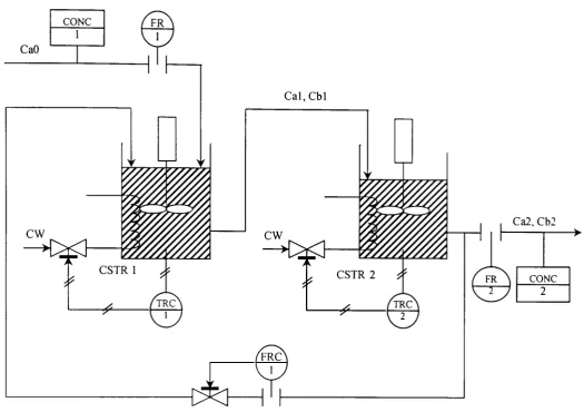
3.3 THE TWO CONTINUOUS STIRRED TANK REACTORS
(CSTR'S)
This example presented by Garcia and Morari (1981) used by lang et al. (1987) and later treated by Becerra and Roberts (1995), consists of two Continuous Stirred Tank Reactors (CSTR's) connected in cascade in which an exothermic autocatalytic reaction takes place (Figure 3-2). The components interact in both
directions due to the recycle of 50% fraction of the product stream into the first
reactor. Regulatory controllers are used to control the temperature in both
reactors.
The reaction is described by the basic reaction equation:
(3.2)
where A and B are two chemical components.
The real process is represented by the following relations:
dCa 2
=
Cal _ C a 2 _ (k C C - k C 2)dt
'2
'2
2+ a2 h2 2- h2dCh2
=
ChI _ C h2 (k C C - k C 2)dt
'2
'2
+ 2+ a2 h2 2- h2(3.3)
(3.4)
(3.5)
(3.6)
Where CXi is the concentration of component x in tank i,
'1
=
30 min is the meanresidence time of reactor 1,
'2
=
25 min is the mean residence time of reactor 2,which result in an overall time constant of approximately 40 min (Garcia and
Morari, 1981). kit
=
A±exp(- E± / RI;) are the reaction rates, E+ / R=
17786K,E_ / R =23523K, A+ = 9.73 x 10²²m3/ kmols, A_ = 3.1 xl 030m3/ kmols, Ca O=0.1 IS
the feed concentration of component A,
1;
is the temperature in tank 1, T2 is thetemperature in tank 2.
CaO
L2
~
Cal, Cbl
Cal, Cb2
CONC 2
Figure (3-2): The two Continuous Stirred Tank Reactors system.
These equations, together with the regulatory control loops, the measurement
transducers and the valve actuators provide the real process description. In our
case, the dynamics associated with the regulatory controllers were neglected as
well as the measurement transducers and actuators (which were originally
modelled as first order lags), as the real system process is a very slow process and
its dominant time constant is very large compared to those of the instrumentation.
There fore, the above equations represent the mapping H* of the real system.
It has to be mentioned that when using the ISOPE algorithm (Chapter 2), an incorrect and simplified model is used as a mapping H to represent the system.
This mapping is different from the one given above.
The two CSTR plant has 4 outputs which are the concentrations of the two
components A and B in both tanks. Hence, the output vector can be written as:
[image:51.713.94.620.130.500.2](3.7)
The manipulated variables which are the set points of the temperature controllers in both reactors are given by,
These are bounded between upper and lower levels:
300 <
1;
<312 K, 300 <T2 < 312 K and are assumed to be known noise free.3.4 IMPLEMENTATION ISSUES
The implementation of the CSTR and the simple SISO systems presented in this chapter was performed using a MATLAB@/SIMULINK software platform.
MATLAB is a high-performance language for technical computing. It integrates computation, visualisation, and programming in an easy-to-use environment where problems and solutions are expressed in familiar mathematical notation. Typical uses include:
• Mathematics and computation • Algorithm development
• Modelling, simulation, and prototyping • Data analysis, exploration, and visualisation • Scientific and engineering graphics
• Application development, including Graphical User Interface (GUI) building.
MA TLAB is an interactive system whose basic data element is an array that does not require dimensioning.
The name MATLAB stands for matrix laboratory. MATLAB was originally written to provide easy access to matrix software developed by the LINPACK and EISPACK projects, which together represent the state-of-the-art in software for matrix computation.
MATLAB features a family of application-specific solutions called toolboxes. Toolboxes are comprehensive collections of MATLAB functions (M-files) that extend the MATLAB environment to solve particular classes of problems.
SIMULINK, a companion program to MATLAB, is an interactive system for simulating both linear and nonlinear dynamic systems. It is a graphical mouse-driven program that allows a system to be modelled by drawing a block diagram on the screen and manipulating it dynamically. It can work with linear, non-linear, continuous-time, discrete-time, multivariable and multirate system (The MathWorks, 1996).
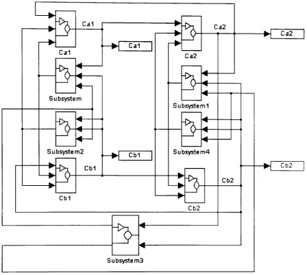
The implementation of both systems was achieved by creating a SIMULINK model architecture which is able to interact with the MATLAB environment via calling a subroutine containing the appropriate identification and optimisation algorithms stored in an M-file. The subroutine acquires the information data under the form of measurements from the SIMULINK model of the plant (figure 3-3). The subroutine is executed at every time sample given in the SIMULINK model parameters, which makes the whole procedure recursive. Major consideration and extra care have to be taken when choosing the simulation parameters. For example, we mention that the time step in a SIMULINK model is not the real time step which means if a measured variable is plotted against time; it would be the internal SIMULINK time not real time. Therefore the time, ODE and the other parameters are to be tuned first before simulation starts. These parameters are chosen following some specific criteria so that the whole system (SIMULINK 1110del and optimisation routine) works in a perfect state.
It is worth noting that the simulation times which appear In the results in subsequent chapters relate to the real plant. The simulations would typically run at speeds of between 10 to 100times faster depending on the computational load on the algorithm; and they are run for suitable time durations, giving time to the
appropriate system to settle down for a steady-state position and for the appropriate algorithms to perform their tasks. All the results are then stored in the workspace to be analysed and plotted.
I
...
....~
~...
Ca1 -,..~
Ca2...
~"'-Ca2 I
-,..
...
--.
~ Ca1 I-+
Ca1
Ca2
~
...
...
...
> -
...
~
...
...
~+-
-
...
~ Subsystem...
Subsystem1~
...
...
...
...
~
...
...
~~+-
~...
Subsystem2 Subsystem4~ Cb1 I
...
~
~ Cb2I
...
Cb1...
--.
"'-~
.... Cb2...
-.
...
~ Cb1 .... Cb2~
...
~...
...
Subsystem3Figure (3-3): SIMULINK implementation example of the CSTR system.
3.5 SUMMARY
[image:54.713.136.585.186.587.2]CHAPTER 4
TECHNIQUES FOR THE ESTIMATION OF
THE DERIVATIVE INFORMATION
4.1 INTRODUCTION
The model-reality differences problem in the general on line optimisation problem is usually overcome by using adaptive models which can be updated regularly while seeking to reach the solution of the optimisation problem. The Integrated System Optimisation and Parameter Estimation (lSOPE) algorithm uses such models. The major drawback the method possesses is the need for derivative information to be estimated at each operating point. These derivatives are needed by the algorithm in order to satisfy necessary optimality conditions (Appendix A).
4.2 FINITE
DIFFERENCE
APPROXIMATION
METHOD
(FDAM)
This method was the first employed for estimation of derivatives (Roberts, 1979) and use is made of process measurements. If the process is subject to noise, then the derivative estimates can suffer large errors giving problems in obtaining the correct final solution. Other difficulties which might arise, apart from those concerned with noise, are the obtaining of actual measurements and, for slow dynamic processes, having to wait for the process to settle sufficiently before steady-state measurements are taken.
In most practical situations, the process mapping is not given by a specific formula or is difficult to find; rather it is a combination of experimental and computational procedures. Thus, the output derivative matrix with respect to the set-points needed by the ISOPE algorithm is usually unavailable.
In one dimensional case, the derivative of a certain function fix) can be replaced by the secant line that goes through
I
at Xc and at some nearby point Xc +h,(Dennis and Robert, 1983). The most obvious formulation of that line slope is:
[t
x;
+
hJ-
l(xJ
a
=
-=---~_.::...---:'--C h
c
(4.1)
Therefore, the output derivative function with respect to the set-point of a given process can be replaced by the following estimation:
al
I(x+
h) - I(x)-ax
h(4.2)
However. will the above formulation be a faithful approximation to the derivative
function off?
The answer comes from the fact that as h goes to zero, ac converges to f'(x). Therefore, h has to be chosen conveniently small so that the estimation (4.2) can be true, and ac can be calledfinite-difference approximation tof'(x).
In the multidimensional case, it is reasonable to use the same idea to approximate
the (ij),h component of the derivative matrix A by the following forward
difference approximation
1;
(x+
heJ ) -1;
(x)a ..
=---....:..----If h (4.3)
where ej denotes the
/h
unit vector. The above formula IS equivalent to approximating ther
column ofA byA = _F_(x_+_he....:c.J_) _F_(x_)
J
h
(4.4)where A is the derivative matrix of the multidimensional function F.
Again, the matrix A converges to the true derivative matrix only ifh is chosen to be sufficiently small.
In practice, and in MIMO (Multi Input Multi Output) systems, the output derivative matrix with respect to the set-points is similarly given by:
D
=
_8y ~ _y_(v..:..:....k _+_g_)_y_(---,vk",--)k