An advanced synthetic eddy method for the computation of aerofoil-turbulence interaction noise

An advanced synthetic eddy method for the

computation of aerofoil-turbulence interaction noise

Jae Wook Kim, Sina Haeri

Aerodynamics & Flight Mechanics Research Group, University of Southampton, Southampton, SO17 1BJ, United Kingdom

Abstract

This paper presents an advanced method to synthetically generate flow tur-bulence via an inflow boundary condition particularly designed for three-dimensional aeroacoustic simulations. The proposed method is virtually free of spurious noise that might arise from the synthetic turbulence, which en-ables a direct calculation of propagated sound waves from the source mecha-nism. The present work stemmed from one of the latest outcomes of synthetic eddy method (SEM) derived from a well-defined vector potential function creating a divergence-free velocity field with correct convection speeds of eddies, which in theory suppresses pressure fluctuations. In this paper, a substantial extension of the SEM is introduced and systematically optimised to create a realistic turbulence field based on von K´arm´an velocity spectra. The optimized SEM is then combined with a well-established sponge-layer technique to quietly inject the turbulent eddies into the domain from the up-stream boundary, which results in a sufficiently clean acoustic field. Major advantages in the present approach are: a) that genuinely three-dimensional turbulence is generated; b) that various ways of parametrisation can be cre-ated to control/characterise the randomly distributed eddies; and, c) that its numerical implementation is efficient as the size of domain section through which the turbulent eddies should be passing can be adjusted and minimised. The performance and reliability of the proposed SEM are demonstrated by a three-dimensional simulation of aerofoil-turbulence interaction noise.

Keywords: , Synthetic eddy method (SEM); Inflow turbulence;

Computational aeroacoustics (CAA); Aerofoil-turbulence interaction (ATI)

noise

1. Introduction

The generation of synthetic turbulent flows is currently one of the chal-lenging issues in computational aeroacoustics (CAA). It has a significant impact on the simulation of important engineering problems such as aerofoil-turbulence interaction noise that is related to turbofan engines, open rotors, wind turbines, helicopters, etc. There are a few crucial properties that a syn-thetic turbulence has to satisfy/offer in order to achieve a successful CAA simulation: 1) divergence-free condition, 2) synchronised convection with the mean flow, 3) statistical characteristics of realistic turbulence and 4) gen-uinely three-dimensional capabilities. Failure to meet all these criteria would result in either spurious noise that contaminates the far-field acoustic data or incorrect source mechanisms at the near field. In addition, the generation of synthetic turbulence should be numerically efficient not to overload the entire simulation.

Over the past years, various techniques of generating synthetic turbu-lence have been proposed and they mostly stemmed from incompressible flows background. Some of them have also been applied to compressible/aeroacoustic calculations, which can be categorised into: a) Fourier modes [1–6], b) ran-dom particle meshes [7, 8] and c) synthetic eddy method (SEM) [9–12]. The Fourier-mode based approach is probably one of the most frequently at-tempted methods for CAA applications due to its simplicity to generate a divergence-free velocity field by taking the cross product of the wavenum-ber and amplitude vectors. The divergence-free condition is crucial for CAA applications to prevent spurious artefact noise that may emerge from the synthetically generated turbulence. However, this is not the only criterion to achieve noise-free turbulence. Sescu and Hixon [12] found that the convection velocity of the synthetically generated turbulence must be synchronized with the local mean-flow velocity in order to guarantee a clean aeroacoustic envi-ronment not interfering with genuine sound waves. Currently the synchro-nized convection has not been considered in the Fourier-mode approaches. In the meantime, the random-particle-mesh approach has demonstrated some promising results for aeroacoustic simulations but a full three-dimensional (3D) extension is yet to be achieved in the near future.

sim-ulations. The recent achievement was made by introducing an eddy shape function (vector potential) and taking the curl of the vector potential to create a divergence-free velocity field, where the argument function of the vector potential was properly determined to satisfy the synchronized convec-tion condiconvec-tion highlighted above. Sescu and Hixon [12] showcased through benchmark tests that the new SEM could potentially be the first successful 3D method for noise-free synthetic turbulence aimed at CAA simulations. There still is a significant scope of work to be done to construct “realistic” turbulence statistics based on the new method and demonstrate its actual performance in a large-scale 3D CAA simulation, which is the main focus of this paper.

In this paper, the latest SEM is combined with a sponge-layer tech-nique [13–15] that was particularly designed for introducing velocity dis-turbances as well as absorbing spurious noise. With this combination, the level of spurious noise is kept sufficiently low to guarantee a clean sound field for CAA simulations. Secondly, new parameters to characterise the ran-domly distributed eddies (i.e. sizes, locations, directional strengths and the population per volume) are introduced and effectively optimized by using Genetic Algorithm to get the resulting turbulence statistics matched with von K´arm´an spectra. It should be noted that the optimisation of the eddy parameters is implemented with inclusion of a periodic boundary condition across the lateral boundaries of the domain. The current periodic boundary condition provides C∞-continuity which yields entirely smooth connection of the two lateral boundaries. Thirdly, the stream of the synthetic eddies is confined within a narrow channel passing through the near-field area only rather than the entire domain. This has a significant impact on the numerical efficiency since otherwise very fine meshes must be maintained throughout the entire domain in order to resolve the smallest eddies that are normally much smaller than the corresponding acoustic wavelengths. Lastly, the op-timized SEM is applied to a 3D simulation of aerofoil-turbulence interaction noise and the results are compared with existing theoretical prediction and experimental data.

is carried out in order to verify its low-noise capability and actual turbulence statistics. Section 6 demonstrates the application of the optimised SEM to a 3D simulation of aerofoil-turbulence interaction noise where the performance and reliability of the proposed approach is addressed. Finally, concluding remarks are given in Sec. 7.

2. Synthetic Eddy Model

The present synthetic eddy method (SEM) is based on a vector potential Ψ(x, t) proposed by Sescu and Hixon [12], which is constructed by superim-posing contributions from randomly distributed vortical eddies. The result-ing velocity field induced by the vortical eddies is obtained by takresult-ing the curl of the vector potential, i.e. u(x, t) =∇ ×Ψ(x, t), which is divergence free. It is suggested in this paper that an artificial turbulence field with realistic velocity spectra can be constructed by imposing certain regularisations and constraints on the sizes, shapes and directional strengths of the randomly distributed eddies in a 3D space. A general form of the vector potential may be written as:

Ψ(x, t) =a_∞

AeLe

Ne

1 3 Ne

i=1

[ψ_x,i(x, t)e_x+ψ_y,i(x, t)e_y +ψ_z,i(x, t)e_z] (1)

where a_∞ is the ambient speed of sound, Le is the length of a “virtual”

eddy box in which the eddies are created, Ae is the eddy box’s cross-section

area through which the eddies are injected into the computational domain (hence AeLe is the volume of the virtual eddy box), Ne is the number of

eddies. (AeLe/Ne)1/3 indicates an average distance between two adjacent

eddies inside the virtual eddy box. ψ_x, ψ_y and ψ_z are a set of dimensionless shape functions for each individual eddy component. e_x, e_y and e_z are the directional unit vectors in the Cartesian coordinate system.

components. The present shape functions are defined as:

ψ_ξ,i(r_i) =

_ξ,iσ_ξ,i−1/2exp[−(3σ_ξ,ir_i)2_{] (Gaussian)}

_ξ,iσ_ξ,i−1/2[1−(4σ_ξ,ir_i)2_{] exp[−(}√_8σ

ξ,iri)2] (Mexican Hat)

∀ξ ∈ {x, y, z} & ∀i∈ {1,· · · , Ne}

(2) with

r_i =r_i(x, t) = (x−x_o,i−u_∞t)2+ (y−y_o,i−v_∞t)2+ (z−z_o,i−w_∞t)2 (3)

where (_x, _y, _z) is an amplitude vector to determine the directional strength of the eddies; (σ_x, σ_y, σ_z) is a set of constants that determines the size of each eddy component; and, xo = (xo, yo, zo) is the centre location of an

eddy. The subscript ξ ∈ {x, y, z} represents each directional component and

i ∈ {1,· · · , Ne} is an index to denote each individual eddy. The argument

function r(x, t) indicates that the eddies move downstream with the mean flow u_∞ = (u_∞, v_∞, w_∞). The Gaussian and Mexican-hat profiles produce various length scales ranging from the eddy diameter all the way down to the grid cell size. The Mexican-hat profile is particularly effective in providing more small scales as shown in Fig. 1.

It is shown in [12] that the arrangement through Eqs. (1) to (3) satisfies the linearised Euler momentum equations and therefore genuinely removes the possibility of causing pressure fluctuations from the synthetic eddies. The divergence-free condition stand-alone is not a sufficient condition for zero pressure fluctuations as mentioned earlier.

3. Creating Realistic 3D Turbulence Based on SEM

Figure 1: Example profiles of velocity spectra created by individual eddies in different sizes with Gaussian (“——”) and Mexican-hat (“– – –”) shape functions, compared with a von K´arm´an spectrum (“–·–” based on 4% integral length scale and 2.5% turbulence intensity). The symbols represent: R = 0.3 (); R = 0.2 (); and, R = 0.1 (+). The eddy radius (R) is defined in Sec. 3.1.

3.1. Parametrisation and Definition

The 15 constraint parameters introduced in this paper for use with Eqs. (1) to (3) are defined and listed in Table 1. In the table, the size of an eddy is defined by R =σ−1/2 _{(approximate radius) deduced from the shape}

func-tions given in Eq. (2). The weighting factor β is introduced to yield a biased eddy distribution towards either the lower (if β >1) or the upper bound (if 0 < β < 1) of the eddy size. The superscript “(0)” is used for representing the Gaussian profile and “(1)” for the Mexican Hat, throughout the paper. The details of how these constraint parameters are used for the creation of the synthetic eddies is shown below.

Once the 15 constraint parameters are determined/found (by using an initial guess and subsequent refinements in an iterative manner – see Sec. 3.4), eight independent random numbers are generated and made available for each individual eddy. The random numbers used here are uniformly distributed between zero and one:

ϕ_n,i∈ U(0,1), ∀i∈ {1,· · · , Ne}, ∀n∈ {1,· · ·,8} (4)

Table 1: Constraint parameters introduced in this paper to optimise synthetic eddies and create realistic turbulence statistics. “G” and “MH” indicating Gaussian and Mexican Hat profiles, respectively as defined in Eq. (2).

Parameters Definitions

Ne Total number of eddies created in a virtual eddy box

Le Length of the virtual eddy box

αg Probability of G-eddies (1−αg: probability of MH-eddies)

R(0) min, R

(1)

min Lower limits in eddy sizes (radii): G (0) and MH (1)

R(0)

max, Rmax(1) Upper limits in eddy sizes (radii): G (0) and MH (1)

β(0)_{, β}(1) _{Weighting for biased eddy distributions: G (0) and MH (1)}

a(0)

x , a(1)x Upper limits in eddy strength inx−direction: G (0) and MH (1)

a(0)

y , a(1)y Upper limits in eddy strength iny−direction: G (0) and MH (1)

a(0)

z , a(1)z Upper limits in eddy strength inz−direction: G (0) and MH (1)

numbers are then linked with the constraint parameters to determine the type, size, coordinate and directional strength of each eddy component as follows:

m_i =

0 if ϕ1,i≤αg

1 if ϕ1,i > αg

, ∀i∈ {1,· · · , Ne}, (5)

⎛ ⎝RRx,i_y,i

R_z,i

⎞

⎠=R(mi) min + (R

(_mi) max −R

(m_i) min )

⎛ ⎜ ⎝

ϕβ_1,i(mi) ϕβ_2,i(mi) ϕβ_3,i(mi)

⎞ ⎟

⎠, (6)

(σ_x,i, σ_y,i, σ_z,i) =R_x,i−2, R−_y,i2, R−_z,i2 , (7)

x_o,i=

xref−κR_x,1 if i= 1

x_o,i–1−κ(Rx,i–1+Rx,i) if i≥2

with κ=Le

Ne

=1

2R_x,, (8)

y_o,i=R_y,iϕ4,i−1₂

, (9)

z_o,i = min(L_z,Lˆ_z)ϕ5_,i− 1₂

with ˆL_z = 3L_z−2 max(R_x,i, R_y,i, R_z,i), (10)

(_x,i, _y,i, _z,i) = a(mi)

x , a(ymi), a(zmi)

·(2ϕ6,i−1,2ϕ7,i−1,2ϕ8,i−1). (11)

Equation (5) selects the type of the eddies between Gaussian (m = 0) and Mexican Hat (m= 1) depending on the probability factor αg ∈[0,1].

numbers (ϕ1, ϕ2, ϕ3) ∈ U(0,1) varying from the lower to the upper bounds

pre-determined earlier. The exponent (weighting factor) β in Eq. (6) drives the eddy distribution towards the upper bound (large sizes for low frequen-cies) if 0 < β <1 or towards the lower bound (small sizes for high frequencies) if β >1. The streamwise locations of the eddies (xo) are given by Eq. (8) in

such a way that the distance between any two adjacent eddies is proportional to the sum of theirx-component radii and that all the eddies are contained in the specified length (Le) of the virtual eddy box. The coordinatexref

repre-sents the forefront position of the virtual eddy box (to be clarified in Sec. 4). Equations (9) and (10) determines the vertical and spanwise locations of the eddies, where |yo| ≤ R_y/2 and |zo| ≤ L_z/2 (L_z: the span of the domain).

This means that the cross-section area of the box is Ae = 3RmaxLz that is

required in Eq. (1). The origin of the coordinate system (x, y, z) = (0,0,0) always refers to the geometric centre of the body (aerofoil) in this paper. The buffer variable ˆL_z in Eq. (10) is introduced to keep the influence of an eddy within |z| ≤3L_z/2 and therefore an efficient construction of a spanwise periodic boundary condition of class C∞ is allowed (see Sec. 3.2). This also means that the size of the largest eddy (Rmax) should be smaller than 3Lz/2.

Lastly, Equation (11) indicates that the directional amplitude and its sign may change randomly within the specified lower and upper limits.

One of the advantages in the present SEM is that the stream of the convecting eddies is narrowed around the body of interest (aerofoil) and its vicinity only, where the size of the stream is controlled by Eq. (9), i.e.

y∈[−1.5Rmax,1.5Rmax]. This helps to minimise the computational overhead

in calculating/storing the inflow velocity signals; removes the necessity to lay out fine meshes in the far field; and, also keeps the far field undisturbed by the flow turbulence for clean aeroacoustic environment.

3.2. Periodic Boundary Conditions

One of the most common boundary conditions used in 3D simulations of aerofoil flows is periodic conditions across the spanwise boundaries. A basic approach to impose such a periodic boundary condition (PBC) when creating a synthetic turbulence field is to use a blending technique, e.g. f(z) =

g(z) +g(L−z) for z ∈ [0, L] which satisfies f(2n)_{(0) = f}(2n)_{(L) for n ≥ 0}

but f(2_n+1)_{(0) = f}(2_n+1)_{(L). The discontinuities (particularly of the first}

of causing dispersive errors (eventually radiating as spurious noise) when numerical differentiation (e.g. a seven-point-stencil central difference) takes place across the boundaries.

In this paper, a spanwise PBC withC∞-continuity is proposed to ensure an artefact-free sound field as a result of the current simulation of aerofoil-turbulence interaction. The proposed strategy to construct the PBC is that the virtual box of eddies is duplicated and repeated on the left- as well as the right-hand side of the original box. The induced velocity profile across the centre box becomes periodic due to the recurrence of eddy distribution across the span. This process does not affect the divergence-free condition which is inherently satisfied for each individual eddy. The spanwise PBC is created by using the following equation:

ΨPBC(x, t) =Ψ(x−Lzez, t) +Ψ(x, t) +Ψ(x+Lzez, t) (12)

where the original vector potentialΨ(x, t) has already been given by Eqs. (1) to (3) and through the procedure described in Sec. 3.1. The spanwise domain is z ∈[−L_z/2, L_z/2]. Equation (12) indicates that the number of eddies and the size of virtual eddy box triple in order to implement the current spanwise PBC. As described in Sec. 3.1 based on Eq. (10), the size of the largest eddy (Rmax) is limited to 3Lz/2 with its centre located at the middle of the span

in order to prevent an eddy in the centre box from reaching beyond the far sides of the neighbouring boxes. This leads to:

Ψ|

z=_±3_2Lz =

∂nΨ ∂zn

z=_±3 2Lz

= 0, ∀n= 1,2,3,· · · (13)

and therefore,

ΨPBC|

z=±L₂z = Ψ|z=−L₂z + Ψ|z=L₂z , (14)

∂nΨPBC

∂zn

z=±L₂z

= ∂

n_Ψ ∂zn

z=−L₂z

+ ∂

n_Ψ ∂zn

z=L₂z

∀n ≥1, (15)

which proves the C∞-continuity of the proposed PBC across the spanwise boundaries.

keeping the computational cost (both CPU time and data storage) at a rea-sonable level and also allowing for efficient post-processing of the simulation data associated particularly with Fourier transformation routines.

3.3. Optimisation Target: von K´arm´an Velocity Spectra

Based on the arrangements described above, an optimisation of the 15 constraint parameters (defined in Sec. 3.1) is performed in order to construct realistic von K´arm´an velocity spectra as a result. The von K´arm´an spectra for a homogeneous isotropic velocity field are given by [17]:

Φ_ij(k) =A(k)

δ_ij −kikj k2

, ∀i∈ {1,2,3} & ∀j ∈ {1,2,3} (16)

with

A(k) = 55L

5

0Γ(5/6)urms2 k2

36π3_/2_{Γ(1/3) (1 +L}2 0k2)

17_/6 & L0 =

Γ(1/3) √

πΓ(5/6)Lt (17)

where k_i’s are wavenumbers, k2 _{= k}

iki, urms2 = u_iu_i/3, Γ is the gamma

function and Lt is the integral length scale. The power spectral density

function for each velocity component can be calculated by

E₁₁VK(k1) = 2

∞

−∞

Φ11(k)dk2dk3, (18)

E₂₂VK(k1) =E33VK(k1) =

1 2

E₁₁VK(k1)−k1

dE₁₁VK dk1

(19)

which yields

E₁₁VK(k1) =

u2 rmsLt

π(1 +L2 0k12)

5/6, E VK

22_,33(k1) =

u2

rmsLt(3 + 8L20k12)

6π(1 +L2 0k12)

11/6 (20)

for the longitudinal and transverse velocity spectra, respectively. The super-script “VK” denotes “von K´arm´an”. In this paperE_iiVK(k1) are multiplied by

a factor of 2 to convert them to one-sided spectra. In addition, the spectra are transformed into a dimensionless frequency domain via:

f∗ = f Lc

a_∞ = k1

whereLc is the reference length in this paper (aerofoil chord) and M∞ is the

free-stream Mach number.

In this work, the velocity spectra required at the position where an aero-foil’s leading-edge would be located are characterised by u_rms/u_∞ = 0.025 (2.5% turbulence intensity) and Lt/Lc = 0.04. These data were obtained

from an experimental measurement of grid turbulence carried out in an ane-choic wind tunnel at the Institute of Sound and Vibration Research (ISVR) of the University of Southampton. The wind speed was u_∞ = 80 m/s (M_∞ = 0.24) and the aerofoil chord wasLc = 15 cm (henceRe∞= 8.6×105

based on u_∞ and Lc). It was confirmed that the measured velocity spectra

matched very well with the corresponding von K´arm´an spectra [18]. Since the synthetic turbulence is generated at the inflow boundary, the target ve-locity spectra at the inlet should be different from those at the aerofoil’s leading-edge position. Under the present numerical set-up, u_rms/u_∞ = 0.04 (4% turbulence intensity) and Lt/Lc = 0.04 are set as the target to achieve

at the inlet, which is found to lead to the desired experimental condition at the aerofoil’s leading-edge position.

3.4. Optimising Eddy Constraint Parameters

Once the target von K´arm´an velocity spectra are identified, an optimisa-tion of the 15 constraint parameters:

φ= (Ne, Le, αg, R(0)min, R (0) max, R

(1) min, R

(1) max, β

(0)_{, β}(1)_{, a}(0)

x , a(0)y , a(0)z , a(1)x , a(1)y , a(1)z )

(22) is carried out in order to find a local minimum of the following L_∞-norm error function:

E(φ) =max3

i=1

f∗

b

max

f∗_=f∗

a

log₁₀Eii(f

∗₎

EVK

ii (f∗)

(23)

with

E_ii(f∗)= 1

L_z

_Lz/2

−Lz/2

E_ii(f∗, z)_(x,y)=(x

min,0)dz (24)

wheref∗ ∈[f_a∗, f_b∗] is the range of frequencies considered in the optimisation. In the current optimisation platform, f_a∗ = 0.1 and f_b∗ = 2.5 are selected, which correspond to 228Hz and 5690Hz, respectively. The numerical spectra

E_ii(f∗,x) are calculated from the vector potential ΨPBC given by Eq. (12)

functionE(φ) returns the largest deviation of the spanwise-averaged numer-ical spectra from the desired von K´arm´an ones within the specified frequency range.

In this work, the number of eddies and the length of the virtual eddy box are fixed at Ne = 300 and Le = 5.76Lc for computational efficiency

although more eddies and a longer box would help improving the result. The time required for an eddy to travel the distance of Le is therefore (in

a dimensionless form) a_∞t/Lc = M_∞−1Le/Lc = 24, which is sufficiently long

for a statistical analysis. In the meantime, the smallest eddy size relative to the aerofoil chord (R(1)_min/Lc) is limited at an affordable level (0.1 in this

work) since the grid density at the inflow boundary should be sufficiently high to resolve the smallest eddy. The rest of the constraint parameters are determined when a gradient-based optimisation technique converges to a local minimum ∂E/∂φ_i = 0 (if failing to find the global minimum) of the error function in Eq. (23). The gradient-based optimisation is accelerated by adopting Genetic Algorithm (via MATLAB Toolbox) and therefore each cycle of the optimisation is completed within a reasonable length of time. The optimisation is repeated with updating the random numbers (ϕ1,· · · , ϕ8)

required in Eq. (4) until the most satisfactory velocity spectra are obtained. It should be noted that Equation (23) is calculated on the horizontal plane (y= 0) that covers the aerofoil planform area, and the Ensemble average of the spectra over the span is taken into account in the iterative optimisation process in order to get sufficiently uniform spectra across the span. The length of span is fixed at L_z/Lc = 0.26 in the present work (see Sec. 6 for

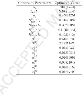
the reason). The resulting constraint parameters revealed at the completion of the optimisation are listed in Table 2.

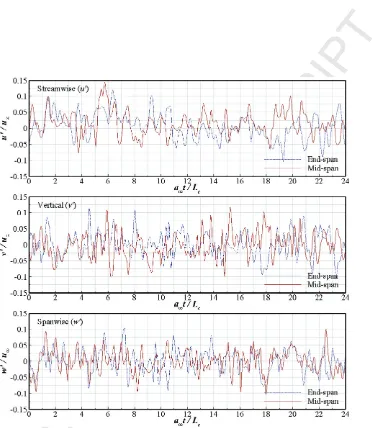
The resulting velocity signals and their spanwise-averaged spectra ob-tained are plotted in Fig. 2 and Fig. 3 for each velocity component. It is shown that the synthetic turbulence spectra are overall in good agree-ment with the corresponding von K´arm´an ones across the frequency range

small-Table 2: Optimised constraint parameters for Eqs. (5) to (11) with spanwise periodic boundary condition based on Eq. (12) and Lz/L_c = 0.26, in order to obtain von K´arm´an velocity spectra at inflow boundary for M_∞= 0.24,u_rms/u_∞= 0.04 andL_t/L_c= 0.04.

Constraint Parameters Optimised Values

Ne 300 (fixed)

Le/Lc 5.76 (fixed)

αg 0.45087254

R(0)

min/Lc 0.14648081

R(0)

max/Lc 0.30203081

R(1)

min/Lc 0.1 (limited)

R(1)

max/Lc 0.19325727

β(0) _0.54655705

β(1) _2.12271470

a(0)

x 0.01509330

a(0)

y 0.01800811

a(0)

z 0.01064091

a(1)

x 0.00821648

a(1)

y 0.01668158

a(1)

est eddies. The extra computational effort, however, might not be critically necessary if there is a sufficient space in the computational domain where the turbulence can travel freely and becomes increasingly realistic after a certain distance from the inflow boundary, which is shown in Sec. 5.3. In the mean-time, it has been checked that the time signals from the two end-span points are identical as expected due to the spanwise periodic condition imposed by Eq. (12).

It should be noted that all the spectra are calculated based on periodic time signals – with the period of T_P∗ = (Le/Lc)/M∞ = 24 – created by the

temporal periodic condition mentioned in Sec. 3.2. The frequency of the periodic turbulence (f_P∗ = 1/24 = 0.04167) is not far from the lowest eddy frequency (f_a∗ = 0.1 set in the current optimisation) albeit still lower by a factor of two. The value off_P∗ can be reduced by extending the length of the virtual eddy box and allocating more eddies in it, which requires a higher computational cost. In the current simulation (aerofoil-turbulence interac-tion), the physics of interest (noise reduction due to a geometric change) takes place at a much higher frequency (f∗ > 1). Therefore, the authors considered that the current value of f_P∗ was adequate in this particular case. However, a more careful consideration will be necessary if a generic flow turbulence is studied where much broader spectra are of interest.

4. Governing Equations and Sponge Layers

This section describes the governing equations that are used for the present simulation of aerofoil-turbulence interaction noise and the sponge-layer technique for absorbing spurious wave reflections as well as injecting the synthetic turbulence into the domain through the inflow boundary. The present governing equations are full 3D compressible Euler equations in a conservative form transformed into a generalised coordinate system:

∂(Q/J)

∂t +

∂(E/J)

∂ξ +

∂(F/J)

∂η +

∂(G/J)

∂ζ =− a_∞

Lc

S

J (25)

where the vectors of conservative variables and fluxes are

Q= ⎛ ⎜ ⎜ ⎜ ⎜ ⎝ ρ ρu ρv ρw ρet ⎞ ⎟ ⎟ ⎟ ⎟ ⎠,E=

⎛ ⎜ ⎜ ⎜ ⎜ ⎝ ρU ρuU+ξ_xp ρvU+ξ_yp ρwU+ξ_zp

(ρet+p)U

⎞ ⎟ ⎟ ⎟ ⎟ ⎠,F=

⎛ ⎜ ⎜ ⎜ ⎜ ⎝ ρV ρuV+η_xp ρvV +η_yp ρwV+η_zp

(ρet+p)V

⎞ ⎟ ⎟ ⎟ ⎟ ⎠,G=

⎛ ⎜ ⎜ ⎜ ⎜ ⎝ ρW ρuW+ζ_xp ρvW+ζ_yp ρwW+ζ_zp

(ρet+p)W

Figure 2: Synthetic turbulent velocity signals obtained at (x, y) = (xmin,0) to be imposed

Figure 3: Spanwise-averaged velocity spectra of the synthetic turbulence obtained at the inflow boundary (x, y) = (xmin,0) based on the parameters listed in Table 2, in comparison

with the internal energy, the contravariant velocities, the coordinate trans-formation metrics and Jacobian given by

et=

p

(γ−1)ρ +

1 2(u

2_+v2_+w2_{), (U, V, W)}T _=A−1_{(u, v, w)}T_,

A−1 = ⎛

⎝ξηx_x ηξy_y ηξz_z ζ_x ζ_y ζ_z

⎞

⎠, J =|A|−1 where A=

∂(x, y, z)

∂(ξ, η, ζ)

.

(27)

The additional terms on the right-hand side of Eq. (25) for the sponge layers suggested in [13, 14] are

S= ⎧ ⎪ ⎪ ⎪ ⎪ ⎪ ⎪ ⎨ ⎪ ⎪ ⎪ ⎪ ⎪ ⎪ ⎩

σs(x, y)

⎛ ⎜ ⎜ ⎜ ⎜ ⎝

ρ−ρ_∞ λs(x)ρ(u−utarget)

λs(x)ρ(v−vtarget)

λs(x)ρ(w−wtarget)

p−p_∞

⎞ ⎟ ⎟ ⎟ ⎟

⎠ for x∈Ωsponge

0 for x∈Ωphysical

(28)

with

σs(x, y) =

σo

2 (1 + cos[πA(x)B(y)]), (29) A(x) = 1−max [(xa−x)/(xa−xmin),0]−max [(x−xb)/(xmax−xb),0],

B(x) = 1−max [(ya −y)/(ya−ymin),0]−max [(y−yb)/(ymax−yb),0],

and

λs(x) = (1 +δ)[1−tanh(x/Lc)] + 1 with δ = min[2M∞/(1 +M∞),1] (30)

where Ωphysical = {x|x ∈ [xa, xb], y ∈ [ya, yb], z ∈ [−1₂Lz,1₂Lz]} defines a

physical domain in which meaningful simulation data are obtained, and the rest of the domain is used as a sponge layer (Ωsponge = Ω∞−Ωphysical)

sur-rounding the physical domain. For the present aerofoil-turbulence interac-tion simulainterac-tion, xa = −5Lc, xb = 6Lc and ya = −yb = 5Lc are selected

and the entire domain is Ω_∞ = {x|x/Lc ∈ [−7,11], y/Lc ∈ [−7,7], z/Lc ∈

[−0.13,0.13]}. The current computational domain set-up is shown in Sec. 5 (see Fig. 4). The overall sponge coefficient is set to σo = 3 in Eq. (29).

Details about the sponge-layer technique can be found in [13, 14].

The target velocity field for Eq. (28) in the sponge layer is specified by

where the heavyside step function that is switched on in the zone of eddy production is defined by

H(x) =

1 for x∈Ωeddy

0 for x∈Ωsponge−Ωeddy

(32)

and the zone of the eddy production is given by

Ωeddy ={x|x∈[xmin, xa] &y∈[−2Rmax,2Rmax]}. (33)

Therefore a small portion of the sponge layer (Ωeddy ⊂ Ωsponge) is used to

inject the inflow turbulence into the domain. The height of Ωeddy is set to

4Rmax which is larger than that of Ae (3Rmax as indicated in Sec. 3.1) in

order to ascertain smooth transition between Ωeddy and Ωsponge. Considering

the vertical distribution (y-coordinates) of the eddies given by Eq. (9), the top and bottom boundaries of Ωeddy are sufficiently distant from the eddies,

where the induced velocity converges to zero, hence smoothly restoring the uniform mean flow u_∞ without discontinuity in Eqs. (28) and (31).

Following up on Sec. 3.1, the parameter xref in Eq. (8) is set to xref = 1

2(xmin +xa +Le) so that the centre of the virtual eddy box is located at

the centre of Ωeddy at the start of the simulation. The time signal of the

eddy-induced velocity is obtained at each grid point in Ωeddy as the virtual

eddy box moves downstream with the mean flow. In practice, two different options of calculating the induced velocity may be considered: 1) instanta-neous values are calculated along with the simulation at each and every time step (and sub-iterative stages between the time steps as necessary); and, 2) a full-length time signal with a reasonable time interval is pre-calculated and stored in a separate binary datafile before the simulation starts which can be accessed fast whenever required. Since Eq. (2) involves exponential oper-ators that are slow in execution, the second option is recommended over the first one although it requires an additional (but not exhaustive) local inter-polation routine. The second option is also beneficial as the same datafile (once created) can be re-used for repeating simulations as far as the meshes remain unchanged inside Ωeddy. In the current computing set-up described

5. Numerical Test of the New Synthetic Turbulence

In this section, the proposed method of 3D synthetic turbulence gen-eration is numerically implemented to test its genuine feasibility for direct aeroacoustic simulations. The primary viewpoint in this section is the level of spurious noise that may develop from the synthetic eddies injected into the computational domain. The eddy vector potential given by Eq. (1) is an exact solution to the linearised Euler equations free of entropy and acoustic perturbations [12]. Applying it to the full nonlinear Euler equations may give rise to the entropy/acoustic waves (spurious noise) in the present simulations. Also, there is a certain level of dispersive errors existing in the numerical so-lution that may radiate as spurious noise as well. The objectives in this section are 1) to ensure that the level of spurious noise is sufficiently low and 2) to find a suitable grid resolution to achieve this. In the meantime, it is checked if the statistics of the synthetic turbulence obtained inside the computational domain matches well with the desired von K´arm´an spectra at the position where an aerofoil is to be placed in the next section.

5.1. High-order Computational Aeroacoustic Simulation

In this work, the full 3D Euler equations with the sponge layers described in Sec. 4 are solved by using high-order accurate numerical methods specif-ically developed for aeroacoustic simulations on structured grids. The flux derivatives in space are calculated based on fourth-order pentadiagonal com-pact finite-difference schemes with seven-point stencils [19]. Explicit time ad-vancing of the numerical solution is carried out by using the classical fourth-order Runge-Kutta scheme with the CFL number of 0.95. The numerical stability is maintained by implementing sixth-order pentadiagonal compact filters for which the cut-off wavenumber (normalised by the grid spacing) is set to 0.87π [20]. In addition to the sponge layers used, characteristics-based non-reflecting boundary conditions [21] are applied at the far boundaries in order to prevent any outgoing waves from returning to the computational domain. Periodic conditions are used across the spanwise boundary planes as indicated earlier.

at the subdomain boundaries. A recent parallelisation approach based on quasi-disjoint matrix systems [22] offering super-linear scalability is used in the present paper. The entire domain Ω_∞ indicated in Sec. 4 is decomposed and distributed onto 312 separate computing nodes/subdomains (26×12×1 in the streamwise, vertical and spanwise directions, respectively). This par-allel computing set-up is maintained throughout the paper.

A snapshot of the resulting pressure (p/p_∞) and velocity (v/a_∞) fields obtained at the end of a test calculation is shown in Fig. 4. The calculation ran up to t∗ =a_∞t/Lc = 80 which is sufficiently long to reach a fully

devel-oped flow (after a transient phase from the initial condition) and to obtain a statistically stationary result when the time signals are sampled for the duration of T_P∗ = 24 indicated at the end of Sec. 3.4. The present synthetic turbulence described in Figs. 2 and 3 is created and injected into the ambient field through the zone of eddy production Ωeddy. The calculation is performed

on a stretched grid with rectangular meshes. The smallest meshes with the size of Δx = Δy = 0.008333Lc (with Δz depending on the number of cells

used in the spanwise direction) are located at (x, y) = (±0.5Lc,0) where an

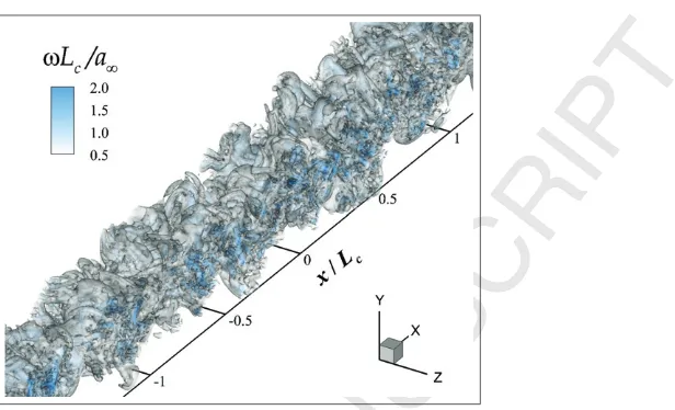
aerofoil will be placed in Sec. 6. The meshes are gradually stretched within the central (near-field) domain and kept almost uniform in the mid- and far-field domain (except the downstream sponge zone). A close-up view on the synthetic turbulence is presented in Fig. 5 based on iso-contour surfaces of vorticity magnitude, where entirely three-dimensional turbulence struc-tures are displayed. It shows randomly coiling worm-like strucstruc-tures which characterise homogeneous isotropic turbulence as reported by Chakraborty

et al. [23].

5.2. Spurious Noise Level

It is shown in Fig. 4 that the resulting synthetic turbulence exhibits very little influence in the far field even at the low contour levels. In order to examine the level of spurious noise that may exist at the far field, the time history of pressure fluctuations is recorded at an observer pointx= (0,5Lc,0)

(point A denoted in Fig. 4) and the normalised power spectral density (PSD) of the sound pressure level (SPL) is calculated as

S_pp(f_n) = 2

p2

∞

_T/2

−T/2

p(t)p(t+τ)e−2πifnτ_{dτ =} 2 T p2

∞

P(f_n) ˜P(f_n) (34)

Figure 4: Contour plots of perturbed pressure (top) and velocity (bottom) fields due to the turbulent stream convecting downstream (left to right) atM_∞= 0.24 in an ambient field. Snapshots obtained ata_∞t/Lc= 80 and taken from anxy−plane at the mid-span (z= 0).

Synthetic turbulence generated within Ωeddybased on 4% intensity (urms/u∞= 0.04) and

4% length scale (Lt/Lc = 0.04) as designed in Sec. 3.4. A total of 24,710,400 grid cells

Figure 5: Iso-contour surfaces of normalised vorticity magnitude ωL_c/a_∞ (ω=|∇ ×u|) obtained from the result shown in Fig. 4. A close-up view around the centre of the domain where an aerofoil is to be placed (see Sec. 6). Four contour levels from 0.5 to 2.

pressure signal is obtained by

P(f_n) = _T/2

−T/2

p(t)e−2πifnt_{dt. (35)}

The factor 2/T in Eq. (34) is required to achieve ₀∞S_pp(f)df =p2_/p2

∞.

The resulting sound pressure spectra are shown in Fig. 6 and the sound pressure level is listed in Table 3. Four different cases with various grid resolu-tion are tested in order to find out the minimum number of grid cells required to resolve the smallest eddies injected into the domain keeping the spurious noise at a tolerable level. The total number of grid cells used for each case is listed Table 4. It is clear from Table 3 and Fig. 6 that the spurious noise decreases as the grid resolution increases, particularly in the mid-to-high fre-quency range. The grid-dependency test does suggest that about 10 cells across Rmin is required to keep the level of the spurious noise sufficiently low

in the mid-to-high frequency range. Henceforth, this criterion (10 cells/Rmin,

i.e. 100 cells/Lc in Ωeddy) is applied to the simulation of aerofoil-turbulence

Figure 6: The PSD of spurious noise generated by synthetic turbulence convecting in an ambient domain. Pressure signals obtained at the observer point A shown in Fig. 4. Four different levels of grid resolution used (Rmin indicating the radius of the smallest eddy

specified in Table 2).

Table 3: The level of spurious noise generated by synthetic turbulence convecting in an ambient domain. Tests with four different levels of grid resolution against the small-est eddy size. Based on pressure signals recorded at the observer point A denoted in Fig. 4.

Minimum number of cells used Resulting spurious noise level

per smallest eddy’s radius (Rmin) (p2/p2_∞)

6 5.157×10−13(71.1dB)

8 3.876×10−13(69.9dB)

10 3.701×10−13_(69.7dB)

12 3.900×10−13(69.9dB)

Table 4: Total number of cells used in the simulation of convecting synthetic turbulence shown in Fig. 4 for four different levels of grid resolution.

Minimum number of cells used Total number of cells used

per smallest eddy’s radius (Rmin) for the entire domain

6 5,778,432 (912×396×16)

8 13,039,488 (1176×528×21)

10 24,710,400 (1440×660×26)

5.3. Mid-domain Velocity Spectra

The synthetic turbulence produced at the inflow boundary region is bound to change due to the interaction between eddies at the integral scale (e.g. vortex dynamics) and eventually develops more realistic turbulence char-acteristics as it convects downstream. In this work, it is aimed to repro-duce the same turbulence statistics at the position (the observer point B at x = (−0.5Lc,0,0) denoted in Fig. 4) where a previous experimental

mea-surement was carried out (mentioned in Sec. 3.3). For this purpose, velocity signals are recorded and their spectra are calculated at the observer point B corresponding to the leading edge of the aerofoil to be located. The resulting spectra are shown in Fig. 7 and they are overall in good agreement with the desired von K´arm´an ones. Also, it is clear by comparing Figs. 3 and 7 that the spectral bandwidth has expanded tof∗ ∈[0.1,5] at the mid domain from [0.1,2.5] that was obtained at the inflow boundary. The improvement in the u spectrum is of particular significance. The expanded bandwidth is attributed to the natural development of the turbulence that takes place as it travels a sufficient distance from the inflow boundary. The effectiveness of the proposed synthetic eddy method is successfully demonstrated.

On another note, the success of synthetic turbulence might also be sured based on how fast the turbulence becomes realistic. This type of mea-sure will be much more relevant in the context of internal flows where the distance that the turbulence travels before turning realistic may be a primary factor to determine the length of the computational domain and therefore significantly related to the cost of the simulation.

6. Application to Aerofoil-Turbulence Interaction Noise

Figure 7: Spanwise-averaged velocity spectra of the evolving turbulence obtained at the observer point B: (x, y) = (−0.5Lc,0) (denoted in Fig. 4), in comparison with the

components associated with viscous effects, e.g. scattering of boundary-layer vortical disturbances inro sound waves at the trailing edge [27].

For the present work, non-lifting thin aerofoils (with zero thickness) with two different leading-edge profiles are considered: a straight (SLE) and a wavy leading edge (WLE). The latter is based on a sinusoidal function of z

(spanwise coordinate) that specifies the local position of the leading edge:

xLE(z) = −1₂Lc+hLEsin [2π(z− 1₂Lz)/λLE] for z∈[−₂1Lz,1₂Lz] (36)

wherehLEand λLEare the amplitude and the wavelength of the leading-edge

profile, respectively. The WLE case is presented in this paper to test and showcase the genuine three-dimensionality of the current approach in both the geometry and the synthetic turbulence. In this paper, hLE = 0.067Lc

and λLE = 0.5Lz = 0.13Lc are selected as were the case in the counterpart

experiment (carried out in the ISVR anechoic wind tunnel mentioned in Sec. 3.3). It has recently been studied by Lau, Haeri and Kim [15] that WLE profiles are effective in reducing ATI noise compared to the SLE case but the existing study relied only on a simple form of vortical gusts (single-frequency velocity excitations). A more comprehensive study based on a realistic 3D turbulence may be achieved by adopting the present SEM approach. It is envisaged that the present result will form an enhanced scope of advanced research associated with ATI noise.

The aerofoil geometries and their surface meshes used in the current sim-ulations are shown in Fig. 8. In both SLE and WLE cases, 660, 120 and 660 cells are used in the upstream; across the chord; and, in the downstream of the aerofoil, respectively. Also, 660 cells are located in the vertical direction (330 above and below the aerofoil each). The total number of cells used is 24,710,400 (with the periodic span covered by 26 cells). This is in fact the same grid set-up used and tested in the previous section for the validation of the synthetic turbulence except that the smallest grid cell size is slightly reduced to Δx = Δy = 0.00625Lc (with Δz = 0.01Lc) at the leading and

trailing edges. Based on the same solution procedure described in Sec. 5.1, the generation and propagation of ATI noise is successfully simulated and the results are plotted in Fig. 9.

Figure 8: Planform views on two different aerofoil geometries and their surface meshes used in the present study. SLE (top) and WLE (bottom). WLE based on Eq. (36) with hLE= 0.067Lc andλLE= 0.13Lc (Lz= 0.26Lc).

levels of Fig. 9 are kept the same as those in Fig. 4 (top), which means that the sound field shown in the current plot do not contain any visible sign of interference due to the spurious noise of the synthetic turbulence. In the meantime, it is apparent in Fig. 9 that the WLE case displays weaker sound waves (particularly for those with small wavelengths, i.e. high frequencies) compared to the SLE case plotted on the same scale. This result does agree with the early investigation by Lau, Haeri and Kim [15].

Sound power spectra obtained at the observer point A (denoted in Fig. 4) for both the SLE and WLE cases are plotted in Fig. 10 where a theoretical prediction by Amiet et al. [24, 28, 29] and an experimental measurement per-formed at the University of Southampton are also included for comparison. It should be noted that the experimental result includes a shear-layer correc-tion and has been scaled up by (rexp/Lc)2/(rsim/Lc) to match the distance

to the observer position and to compensate the 3D decaying rate (p_3D ∝r&

p_2D ∝√r).

em-Figure 9: The result of ATI noise simulation obtained at a_∞t/Lc = 80 and taken from

an xy−plane at the mid-span (z = 0). For two different aerofoil geometries: SLE (top) and WLE (bottom). Based on the synthetic turbulence shown in Fig. 7. Same contour levels for both cases up to ±2×10−4_{. The location of the aerofoil (of zero thickness) is}

ploying more eddies (and increasing the size of the virtual eddy box) as men-tioned at the end of Sec. 3.4, the authors see the current set-up reasonably accurate and efficient for the study of ATI noise and its reduction mecha-nisms associated with WLE. The effect of WLE is evident in the bottom graph of Fig. 10 where both the simulation and the measurement manifest significant noise reduction (by up to 10dB) particularly in the high-frequency range. It should be noted that the measurement data (particularly in the WLE case) contained a noticeable level of self-noise contributions that seem to have led to a flatter broadband spectrum with a little higher level in the high-frequency range compared to the simulation data. Finally, Fig. 11 is plotted to re-confirm that the spurious noise due to the present synthetic turbulence is sufficiently negligible (20 to 60dB lower than the ATI noise in the entire frequency range resolved).

7. Conclusions

Figure 11: The level of spurious noise generated by the present synthetic turbulence in comparison to those from the physical mechanism of ATI noise.

discrepancies were attributed to the fact that the current velocity spectra were not entirely smooth as those in the counterpart theory and experiment. There is a scope of work in the future to refine the velocity spectra without an excessive increase in the eddy population overburdening the computa-tional cost. In conclusion, the present work offers a solid ground on which numerical simulations can now provide highly reliable data to discover and explain the control mechanisms of ATI noise associated with wavy leading edges.

Acknowledgement

[1] R. H. Kraichnan, Diffusion by a random velocity field, Physics of Fluids 13 (22) (1970) 22–31.

[2] A. Smirnov, S. Shi, I. Celik, Random flow generation technique for large eddy simulations and particle-dynamics modeling, Journal of Fluids En-gineering 123 (2) (2001) 359–371.

[3] P. Batten, U. Goldberg, S. Chakravarthy, Interfacing statistical tur-bulence closures with large-eddy simulation, AIAA Journal 42 (2004) 485–492.

[4] A. Keating, U. Piomelli, Synthetic generation of inflow velocities for large-eddy simulation, 34th AIAA Fluid Dynamic Conference and Ex-hibit, Portland, Oregon, aIAA Paper 2004-2547, 2004.

[5] S. H. Huang, Q. S. Li, J. R. Wu, A general inflow turbulence generation for large eddy simulation, Journal of Wind Engineering and Industrial Aerodynamics 98 (10-11) (2010) 600–617.

[6] R. Yu, X. S. Bai, A fully divergence-free method for generation of in-homogeneous and anisotropic turbulence with large spatial variation, Journal of Computatioinal Physics 256 (2014) 234–256.

[7] R. Ewert, Broadband slat noise prediction based on CAA and stochastic sound sources from a fast random particle-mesh (RPM) method, Com-puters & Fluids 37 (2008) 369–387.

[8] M. Dieste, G. Gabard, Random particle methods applied to braodband fan interfaction noise, Journal of Computational Physics 231 (2012) 369– 387.

[9] N. Jarrin, S. Benhamadouche, D. Laurence, R. Prosser, A synthetic-eddy method for generating inflow conditions for large-synthetic-eddy simulations, International Journal of Heat and Fluid Flow 27 (4) (2006) 585–593.

[10] M. Pamies, P. E. Weiss, E. Garnier, S. Deck, Generation of synthetic turbulent inflow data for large eddy simulation of spatially evolving wall-bounded flows, Physics of Fluids 21 (045103) (2009) 1–15.

[12] A. Sescu, R. Hixon, Toward low-noise synthetic turbulent inflow condi-tions for aeroacoustic calculacondi-tions, International Journal for Numerical Methods in Fluids 73 (12) (2013) 1001–1010.

[13] J. W. Kim, A. S. H. Lau, N. D. Sandham, Proposed boundary conditions for gust-airfoil interaction noise, AIAA Journal 48 (11) (2010) 2705– 2710.

[14] J. W. Kim, A. S. H. Lau, N. D. Sandham, CAA boundary conditions for airfoil noise due to high-frequency gusts, Proceedia Engineering 6 (2010) 244–253.

[15] A. S. H. Lau, S. Haeri, J. W. Kim, The effect of wavy leading edges on aerofoil-gust interaction noise, Journal of Sound and Vibration 332 (2013) 6234–6253.

[16] T. S. Lund, X. Wu, K. D. Squires, Generation of turbulent inflow data for spatially-developing boundary layer simulations, Journal of Compu-tational Physics 140 (1998) 223–258.

[17] A. S. Monin, A. M. Yaglom, Statistical fluid mechanics: mechanics of turbulence, vol. 2, MIT Press, 1975.

[18] V. Clair, C. Polacsek, T. L. Garrec, G. Reboul, M. Gruber, P. Joseph, Experimental and numerical investigation of turbulence-airfoil noise re-duction using wavy edges, AIAA Journal 51 (11) (2013) 2695–2713.

[19] J. W. Kim, Optimised boundary compact finite difference schemes for computational aeroacoustics, Journal of Computational Physics 225 (2007) 995–1019.

[20] J. W. Kim, High-order compact filters with variable cut-off wavenumbers and stable boundary treatment, Computers & Fluids 39 (2010) 1168– 1182.

[21] J. W. Kim, D. J. Lee, Generalized characteristic boundary conditions for computational aeroacoustics, AIAA Journal 38 (11) (2000) 2040–2049.

[23] P. Chakraborty, S. Balachandar, R. J. Adrian, On the relationships between local vortex identification schemes, Journal of Fluid Mechanics 535 (2005) 189–214.

[24] R. K. Amiet, Acoustic radiation from an airfoil in a turbulent stream, Journal of Sound and Vibration 41 (1975) 407–420.

[25] M. E. Goldstein, Unsteady vortical and entropic distortions of potential flows around arbitrary obstacles, Journal of Fluid Mechanics 89 (1978) 433–468.

[26] J. W. Kim, D. J. Lee, Generalized characteristic boundary conditions for computational aeroacoustics, part 2, AIAA Journal 42 (1) (2004) 47–55.

[27] R. D. Sandberg, N. D. Sandham, Direct numerical simulation of tur-bulent flow past a trailing edge and the associated noise generation, Journal of Fluid Mechanics 596 (2008) 353–385.

[28] M. Roger, S. Moreau, Extensions and limitations of analytical airfoil broadband noise models, International Journal of Aeroacoustics 9 (3) (2010) 273–305.