The Application of Adaptive Linear and N on-Linear Filters to Fringe Order Identification in White-Light Interferometry Systems

(1)

City, University of London Institutional Repository

Citation

:

Romare, Dario (1998). The Application of Adaptive Linear and N on-Linear Filters to Fringe Order Identification in White-Light Interferometry Systems. (Unpublished Doctoral thesis, City, University of London)

This is the accepted version of the paper.

This version of the publication may differ from the final published

version.

Permanent repository link:

http://openaccess.city.ac.uk/19993/

Link to published version

:

Copyright and reuse:

City Research Online aims to make research

outputs of City, University of London available to a wider audience.

Copyright and Moral Rights remain with the author(s) and/or copyright

holders. URLs from City Research Online may be freely distributed and

linked to.

(2)

The Application of Adaptive Linear and

N on-Linear Filters to Fringe Order Identification

in White-Light Interferometry Systems

Dario ROMARE

A Thesis Submitted for the Degree of Doctor of Philosophy

CITY UNIVERSITY

Department of Electrical, Electronic and Information Engineering

(3)

.

. . .

129

139

139 139 140 145 148 149 154 161

170

170 172

180

185

(6)

List of Tables

3.1 Condition numbers of data matrix used by batch algorithms . . 54 3.2 Condition numbers of data matrix used by adaptive algorithms. 54

5.1 Computer time for sub-fringe identification .

...

"

..

113

7.1 Success rate in white Gaussian noise

...

145

7.2 Success rate in broad-band Gaussian noise 145

7.3 Success rate in narrow-band Gaussian noise 145

(7)

List of Figures

1.1 Output intensity with a He-Ne laser source. 5

1.2 Typical spectrum of an AIGaAs LED 6

1.3 Output intensity with a LED source. 6

1.4 Schematic diagram of a WLI system . . . 8 1.5 Simulated output intensity of a WLI system with noise at 20 dB 11 1.6 Success rate from direct fringe visibility.

2.1 ARMA process driven by white noise .. 2.2 Spectrum of the fringe pattern in Fig. 1.5 2.3 ACS and PACS of the fringe pattern in Fig. 1.5

3.1 FIR adaptive transversal filter . . . . 3.2 Flowchart for on-line prediction with the LMS algorithm 3.3 Flowchart for on-line prediction with the RLS algorithm 3.4 Flowchart for on-line prediction with the Kalman filter . . 3.5 Success rate with batch and adaptive algorithms . . . .

4.1 Success rate with the LMS algorithm against SNR . 4.2 Maximum success rate against filter order

4.3 Success rate against J1. and SNR . . . . 4.4 Success rate against central fringe position

4.5 LMS MSE across the CCD array with a SNR of 32 dB 4.6 LMS MSE with a SNR of 20 dB .

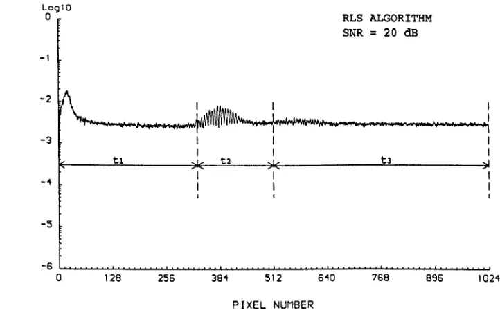
4.7 LMS MSE with a SNR of 10 dB . 4.8 LMS weights with a SNR of 32 dB 4.9 LMS weights with a SNR of 20 dB 4.10 LMS weights with a SNR of 10 dB 4.11 RLS MSE with a SNR of 20 dB .

12

19

25

26

40

41

44

46 48

61

62 62 64 64 65 66 67 67

(8)

4.12 RLS weights with a SNR of 20 dB . . . 68 4.13 Experimentally obtained white-light fringe pattern. 70 4.14 Fringe pattern filtered by the LMS (J.L = 0.1) . 71 4.15 Fringe pattern filtered by the LMS (J.L = 0.01) 72 4.16 Fringe pattern filtered by the RLS (,\ = 1.0) 72 4.17 Fringe pattern filtered by the RLS (,\

=

0.8) 73 4.18 Success rate against coherence length . . . . 79

5.1 Success rate with the thresholded technique 90 5.2 Success rate against central fringe position . 91

5.3 Position of AR(2) model poles against SNR 93

5.4 Diagram showing difference between FB-LMS and MFB-LMS 98 5.5 Success rate with the thresholded MFB-LMS . . . 100 5.6 MSE with the thresholded MFB-LMS (J.L

=

10-3) 102

5.7 MSE with the thresholded MFB-LMS (J.L = 10-6) 102 5.8 Success rate with the centroid method against central fringe position 109 5.9 Success rate with the centroid and covariance methods

5.10 Success rate with the LMS predictors over 992 pixels 5.11 Success rate with the LMS predictors over 960 pixels 5.12 Success rate with the RLS predictor.

5.13 Success rate with the matched filter.

7.1 Density of the central 26 fringes of Fig. 4.13 7.2 Two common ADC non-linearities . . . . 7.3 Fringe pattern distorted by a quadratic non-linearity 7.4 Fringe pattern distorted by a cubic non-linearity. 7.5 Fringe pattern modified by chromatic aberrations

7.6 AR model signal generator and FIR adaptive non-linear filtering . 7.7 Performance of linear and Volterra filters . . . .

7.8 Performance of linear and Volterra filters . . . .

110 110 111 112 112

(9)

Acknowledgements

I wish to thank Dr. M. Sabry-Rizk and Prof. K. T. V. Grattan for their excellent supervision and encouragement throughout the whole PhD research, and Dr. A.

W. Palmer and Dr. Y. N. Ning for the many valuable suggestions.

I am also indebted to Dr. K. Weir, now at Imperial College, University of London, for the patient help and technical assistance provided during the acquisition of experimental data.

(10)

Declaration

(11)

Abstract

Conventional optical interferometry systems driven by highly coherent light sources have a very short unambiguous operating range, a direct consequence of the flatness of the interference fringes visibility profile at the output of the system.

The range can be extended by using a white-light interferometer (WU), which is driven by a low-coherence source and produces a Gaussian visibility profile with a unique maximum in correspondence of the central fringe.

Due to system and/or measurement noise, however, the position of the maximum (from which an accurate measurement of the measurand - displacement, temperature, pressure, flow, etc. - can be derived) is not easily detectable, and can lead to large measurement errors. This is especially true in a multiplexing scheme, where the source power is distributed evenly among various sensors, with a corresponding drop in the overall signal-to-noise ratio. The inclusion of a signal processing scheme at the receiver end is thus a necessity.

As the fringe pattern at the output of a WLI system is basically a noisy sine wave amplitude modulated by a Gaussian envelope, it can be classified as a non-stationary, narrow-band, linear but non-Gaussian signa\. So far, no attempt has been made to apply digital filtering techniques, as understood in the signal processing community, to the output signal of a WLI system. This thesis constitutes a first step in that direction.

Since the only measurable information given by the system is contained in the output signal, the system is modelled as a "black box" driven by the system and measurement noise processes and containing an unknown set of parameters. Standard least squares techniques can then be applied to estimate the parameters of the model, as is usually done in the field of system identification when only noisy output measurements are available.

It is shown that identification of the model parameters is equivalent to finding a set of coefficients for an inverse filter which takes the WU signal at its input and delivers the unknown noise process at the output.

The non-stationarity of the signal is accounted for by allowing for time variations of the model parameters; this justifies the use of adaptive filters with time-varying coefficients. A new central fringe identification scheme is proposed, based on a modification of the standard least mean square (LMS) adaptive filtering algorithm in combination with amplitude thresholding of the fringe pattern. The new scheme is shown to offer considerable improvement in the identification rate when tested against current schemes over comparable operating ranges, while retaining the computational simplicity and operational speed of the standard LMS. Its performance is also shown to be largely independent of the step-size parameter controlling the rate of convergence and tracking in the standard LMS, which is known to be the main obstacle for a successful application of the algorithm in a practical setting.

The non-Gaussianity of the signal is explored and an attempt is made to apply higher-order statistics (HOS) algorithms to central fringe identification. The effectiveness of Gaussianity tests on pilot Gaussian data is seen to depend not only on the number and length of records available but, perhaps more importantly, on the bandwidth of the process. Violation of the stationarity assumption is shown to lead to mis-classification of a seemingly non-Gaussian signal into a Gaussian one, as the visibility profile may alter the distribution of the underlying sinusoid making it appear Gaussian, even when beam diffraction and wavefront aberrations combine to produce a non-Gaussian profile. HOS-based adaptive algorithms may still be of some benefit, however, if processing is confined to that region of the fringe pattern where sufficient non-Gaussianity is allowed to develop.

Non-linear adaptive filters based on the Volterra theories are finally applied to compensate for possible non-linearities introduced by mismatches in optical components, chromatic aberrations, and analogue-to-digital converters. It is shown that although a Volterra filter is able to reproduce the low-amplitude distortions of the fringe pattern better than a linear filter does, the identification rate does not improve. Reasons are given for such behaviour.

(12)

Chapter

1 White-Light Interferometric

Systems

1.1 Introduction

This chapter explains the two main properties of light which are exploited in optical measurement systems, i.e., interference and coherence. The advantages of white-light over monochromatic sources which are responsible for the recent interest in a11-optical-fibre white-light interferometric systems are also described, before examining the central fringe identification problem and the techniques that have been proposed to ease it.

In Chapter two it is shown how a physical system, in this case an optical inter-ferometer, can be approximated by a statistical model consisting of a "black-box" driven by an unknown random process and containing an arbitrary number of pa-rameters. Identification of the central fringe is then formulated as an inverse filtering problem, and known off-line or batch schemes are presented to solve for the filter coefficients.

Adaptive filters, which give rise to on-line schemes, are introduced in Chapter three. A preliminary evaluation of off and on-line filtering algorithms for central fringe identification is presented, using simulated data. An appreciation of

(13)

filtering algorithms, the standard least mean squares (LMS) and the recursive least squares (RLS).

A novel scheme using a modified version of the LMS is presented in Chapter five, which offers a much higher identification rate than that possible with the standard version, at no extra computational cost. The novel scheme is shown to approach the performance limit imposed by the matched filter, which is the ideal solution for the detection of a known signal in additive white noise, and makes the choice of the step-size parameter which controls the convergence and tracking rates in the LMS practically redundant. A comparison between the most commonly used methods for white-light central fringe identification and some of the schemes presented here ends the chapter, with greater emphasis being put on performance and computational complexity.

Chapter six contains a round-up of adaptive filtering algorithms that have not been considered in this thesis but may nevertheless be capable of improving the identification rate offered by the novel LMS scheme, on condition that they are modified along the lines of the novel LMS.

Linear filters based on higher-order statistics are examined in the first part of Chapter seven. Non-linear filters based on the Volterra theories follow, to ac-count for non-linearities introduced by the optical system and by data-acquisition or recording instruments. It is shown that there is at present no reason to prefer a non-linear to a linear filter in current white-light interferometry measuring systems, and the advantage of using higher-order statistics for linear filtering is also doubtful. Chapter eight is a summary of what has been achieved in the field of white-light interferometry by this thesis, and suggests possible extensions that may be worth of further study.

1.2 Optical Interferometry

Optical interference is the phenomenon which can be observed when coherent light from a source is divided into two beams which are then superposed. In the region of superposition, the resultant intensity at different points varies between maxima which exceed the sum of the component intensities, and minima which may be zero.

(14)

have division of wave-front; if, instead, the beam is split at one or more surfaces, at which part of the light is transmitted and part reflected, we have division of amplitude. The first method is only useful with small aperture sources, hence the second method is in general preferable since it gives greater interference effects [1]. Irrespective of the method used, optical interferometry exploits the fact that, for an ideal monochromatic source with wavelength in air Ao, the phase difference between the two beams in the region of superposition is

0= ko6L (1.1)

where ko = 271"/ Ao is the wave number and 6L is the difference between the optical paths through which the two beams have travelled before being recombined 1.

If I is the intensity of the light source, the resultant intensity after recombination can be expressed as [1]

I

Ires = '2(1

+

cos 0) (1.2)

Hence, when 6L is an integral multiple of the source wavelength Ao, 0 is an integral multiple of 271" and Ires reaches its maximum value; conversely, when &L is an odd multiple of half the wavelength, Ires goes through minima equal to zero.

The variation of the output intensity Ires with 0 is often referred to as a fringe pattern because when observed visually it appears as a succession of evenly spaced white and dark fringes.

1.3 Interferometric Systems as Sensors

Optical interferometers come in various forms and shapes, but they all share the same principle.

Those based on amplitude division usually consist of an extended source which is divided into two beams of equal intensities at a beam splitter. The two beams are recombined after reflection at two plane mirrors, and sent to a detector which responds to Ires. If both mirrors are fixed, 8L is constant and so is Ires, but if one of the mirrors is allowed to move, &L varies and Ires with it.

The Michelson interferometer is most often used for the accurate measurement of displacements. The movable mirror is attached to the measurand, and if a

displace-lThe wave number is defined as 1/>'0 in [2], and is the number of waves/em path in vacuum,

(15)

ment of the fringe pattern by m orders has occurred, the movement has introduced an optical path difference (OPD) equal to mAo in air, or

mAo/n

in a medium such as an optical fibre with refractive index n. The displacement of the measurand, d, is given directly as

d= ~mAo

2 n (1.3)

Displacements of up to one-fiftieth of a fringe can be detected, making it possible to perform measurements with an accuracy of one-hundredth wavelength, correspond-ing to 5

nm

for green light [2].

The Jamin, Mach-Zehnder, and Rayleigh interferometers may be used to mea-sure variations of density in gas flows, exploiting the dependence between gas density and refractive index. If t is the thickness of the gas flow traversed by the beam in one arm of the interferometer and the refractive index of air is taken to be unity,

{n - l)t/Ao

extra waves are introduced by the passage of the gas. Hence, if a displacement of the fringe pattern by m orders has occurred, n is obtained from

(n - l)t

=

mAo (1.4)

from which the gas density can be derived.

The main advantage of optical sensors over electrical sensors is their immunity to electromagnetic interference. Their use is increasing all the time and includes such diverse fields as air temperature monitoring, torque measurements, and inho-mogeneity observations in glasses. A detailed account is beyond the scope of this thesis and is widely available in the literature (see, e.g. [3]).

1.4 Temporal Coherence and Coherence Length

(16)

Another way of explaining this phenomenon is to think of the source as consisting of wave trains of finite length. If, after division at the glass plate the OPD between the two halves of each wave train is greater than this length, there is no interference because the two halves being combined are no longer derived from the same wave train, and have lost any correlation to each other [2].

The need for partially monochromatic light is called the temporal coherence requirement for interference [4], and the maximum 8L over which interference effects can be observed is called coherence length. It turns out that the sharper the line width of the source, 8,X, the more monochromatic the light, and the greater the coherence length Le, according to the equation

(1.5)

where

AO

is the mean wavelength [1].

What is more, the fringe profile is the Fourier transform of the spectrum of the light source [5], and this gives a quick tool for predicting interference effects.

1.5

1.0

>-

I-~

Ul 0.5

z

LU I

-Z

~

0.0

0

LU (J)

~

- l

< -0.5

I:

~

a

z

-1.0

-1.5

OPTICAL PATH DIFFERENCE

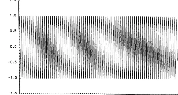
Fig. 1.1 Output intensity with a He-Ne laser source. Lc = 1000 m, corresponding to 1.58 x 109

fringes.

[image:16.513.104.484.392.594.2]

(17)

visibility reduces to lie of its maximum [8]. Hence, the visibility as a function of

8L decays very slowly, giving an output intensity as in Fig. 1.1, which in practice can be approximated by Eq. 1.2.

)0I

-c.n 0.75

z

UJ

I-Z

L

< _0.50

UJ

CD 0

UJ

c.n

--I

< _0.25

L

O!

a

z

WAVELENGTH < nm)

Fig. 1.2 Typical spectrum of an AIGaAs LED, emitting at a central wavelength of 840 nm with

a spectral half-width of 49.4 nm.

c.n

z

UJ

I-Z

o

UJ

c.n

--I

1.5

1 .0

0.5

0.0 f . . - - - " " " " f I / \ / \

;§ -0.5

0::

o

Z

-1.0

OPTICAL PATH DIFFERENCE

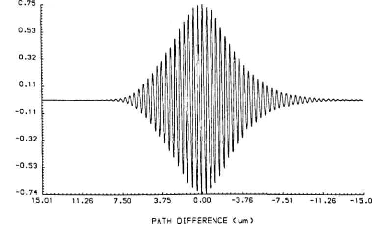
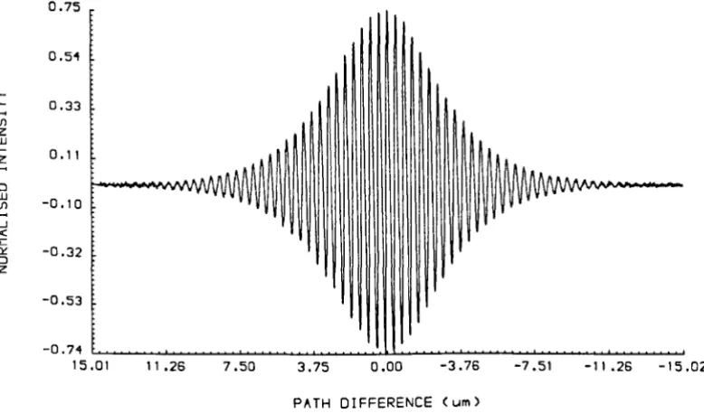
Fig. 1.3 Output intensity of an interferometer with a LED source, obtained by adding 201

[image:17.517.86.475.135.370.2] [image:17.517.103.487.446.657.2]

(18)

In contrast, light-emitting diodes (LEDs) and multimode laser diodes operated below threshold are polychromatic sources with a broad-band Gaussian spectral distribution and a spectral half-width ranging from 20 to 80 nm [9], as in Fig. 1.2. As the Fourier transform is a linear operation, the fringe visibility is also a Gaussian function, as in Fig. 1.3, and the coherence length may only reach a few p,m.

1.5 White-Light Interferometry

The apparent inconvenience caused by polychromatic light sources can be turned to advantage by exploiting the following limitations associated with the use of high-coherence laser devices [10]:

• Unambiguous operating range corresponding to only one wavelength, which in the case of position and distance measurements allows a maximum movement of the measurand by half a wavelength ( Eq. 1.3 ) .

• The inability to identify the interference order when the interferometer is switched off and on.

These limitations are due to the long coherence length of a laser source, which generates a very flat visibility profile and makes it extremely difficult to monitor the movement of the fringes, unless complex and expensive fringe-counting methods are used [11].

When using a source with a short coherence length, the input spectrum is ap-proximately Gaussian, hence the output fringe pattern is the cosine function in Eq. 1.2 modulated by a Gaussian visibility profile. There is then a central white fringe corresponding to the monochromatic fringe of order zero, with a few coloured maxima and minima on either side. The central fringe will remain identified if the power supply is suspended temporarily, either accidentally or on purpose.

A white-light interferometer (WLI) is an interferometric system which uses a polychromatic source and usually consists of two interferometers in series [12, 13]. Referring to Fig. 1.4, the interferometer on the left (called the sensor) can be preset to introduce a path difference

c5L

1 between its two arms much greater than

the coherence length

Lc

of the source

S,

by adjusting the movable mirror

M

2• With

(19)

cannot interfere. Upon reaching the interferometer on the right (the reference or scanner) wave train Ll is split into _L13and L14 at the beam-splitter _B2,while L2 is split into _L23and _L24.Although the two wave trains reflected from the fixed mirror

M3 cannot interfere, and neither can the two wave trains from the movable mirror M_{4, L13}can interfere with L14 and L23 can interfere with L24 if the path difference 8L2 between the two arms of the reference is within Le. The real advantage of using such an arrangement, however, is that _L13can interfere with L24 (or _L23interfere with L 14 ) when 8L2 is equal to 8L1 to within Le. This allows to operate over a range much larger than that imposed by L_{e ,}and which is now dictated only by the scanning range of the reference interferometer.

~s

1

L13 + +L23

Af2 M4

L2 L24

-

...

-

...

Ll L14

t

Fig. 1.4 Schematic diagram of a WLI system consisting of two Michelson interferometers. During the calibration phase, the reference is adjusted to match 8L₂ to 8L_{1 •} During the measurement or sensing phase, the interference fringes will disappear from the detector D whenever the change in 8L1 induced by the measurand in the

sensing interferometer is greater than Le. By scanning the reference, the change in 8L1 can be matched by an equal change in 8L2 , thus restoring the interference

pattern.

(20)

The scanning can be either temporal, using a mechanical or piezo-electrical device, or spatial, using an electronic scanner [14]. With the latter, the reference interferometer produces the fringes by expanding and overlapping the beams from the two arms at an angle on a charge-coupled device (CCD) array. Compared with mechanical scanners, electronic scanners are much faster, more accurate and stable, and have smaller size. Compared with piezo-electric scanners they have a much larger operating range and do not need a high voltage driver [15]. Since no mechanical moving parts are present, their compactness and rigidity makes them especially useful for applications in harsh environments [8].

1.6 Fibre-Optic Interferometric Sensors

An additional advantage of white-light interferometry is that only the sensing unit needs to be in the sensing area, as long as the optical signal can be transmitted back to the reference interferometer. This makes it possible to take measurements in hazarduous and hostile environments, and is one of the reasons for the recent interest in fibre-optic sensors, which offer more safety, reduced weight, and are more resistant to high-temperatures [9].

Such sensors exploit the fact that the OPD in a fibre is affected by its temper-ature, and also changes with pressure and stretching, or when an electric or mag-netic field is applied. Fibre optic sensors using white-light interferometry have been developed, among others for the measurement of absolute displacement [13, 16], refractive index [17], pressure [9], and temperature [18]. In particular, with an all-fibre arrangement, where the beam splitters are replaced by optical-fibre cou-plers, high sensitivity can be obtained, as it is possible to have very long paths in a small space. A considerable reduction in noise can also be achieved because of the immunity of the system to perturbations in the transmission medium [10].

(21)

com-mon optical bus bar and back onto the same busbar to one reference interferometer, where the individual interference patterns can be recovered by coherence multiplex-ing [19, 20]. If the optical delays from each sensor are sufficiently spaced so that no mixing of the light beams occurs in the busbar, in fact, each individual signal can be recovered in turn by scanning the reference over its full range.

1.7 Digital Signal Processing

The normalised fringe pattern at the output of a WLI system can be expressed, after sampling, as follows [8]

sin] = exp [-

(k:~,8,)

}OS(kn -

8,) (1.6)

where n denotes a sample point, Os and kn are the phase differences in the sensing and reference interferometers, respectively, with k being equal to 211" /b, where b is the number of samples per fringe or fringe width, and Lc is the number of fringes within the coherence length.

When kn

=

Os, a perfect matching between the OPDs of the two interferometers is achieved, giving maximum interference contrast.

For a given system setup, Lc and b are fixed parameters; on the other hand, Os may change from one scan to the next according to the measurand, like a random variable uniformly distributed across the scanning range. Hence, the output at an arbitrary point

n

is a particular realisation of a random process

{s[n]}.

Neverthe-less, having observed the sample function

s[n]

one has no difficulty in determining the unknown Os from Eq. 1.6; all that is needed is to look at the sample point corresponding to the maximum value, and equate Os with kn. In this respect, Eq. 1.6 provides a deterministic description of the system.

In the presence of noise, however, the explicit mathematical relationship between system output and phase difference works but with a certain level of error, and it is the uncertainty in deriving the latter that will justify referring to the WLI system as a stochastic system in this thesis.

(22)

Misalignment and offset between the axis of the measurement transducer and the target displacement, optical mixing between the polarisation states of the source caused by imperfect or tilted components, diffraction and wavefront aberrations, changes in refractive index induced by temperature and pressure [21], and shot and thermal noise at the detector all contribute to make identification of the central fringe a difficult task.

These problems are exacerbated in fibre-optic systems because of the low power-coupling between the source and the fibre. Furthermore, vibrations during scan-ning bring the overall signal-to-noise ratio (SNR) down to 40-60 dB in temporally scanned systems

[8].

For electronically scanned systems, on the other hand, the lim-ited spatial coherence of the source reduces the visibility profile as the two beams are brought together at an angle on the CCD array, pushing the SNR further down to 20-40 dB [20].

0.8 0.6 )0- 0.1

I

-(J)

z 0.2 UJ I-Z

-

0.0 0 UJ (J)

-

....J -0.2

<

I:

cr:

0 -0.4 Z

-0.6

-0.8

FRINGE WIDTH=12.70 NUMBER OF FRINGES=17

0 128 256 381

t

512

CENTRE FRINGE AT PIXEL 512 SNR=20 dB

N=1024

6'\0 768 896 1021

PIXEL NUMBER

Fig. 1.5 Simulated output intensity of a WLI system with additive noise at 20 dB. The arrows point at the central fringe.

In the following, the SNR (in dB) is defined as 20Iog(A/0'), where A is the amplitude of the noise-free central fringe and 0' is the root mean square of the

noise, assumed stationary [22]. A SNR of 20 dB, for example, means that noise and central fringe amplitude are in the ratio 1:10.

(23)

Gaussian noise at 20 dB. The coherence length corresponds to 17 fringes and a CCD array consisting of 1024 pixels was assumed for the detector.

Fig. 1.6 shows the percentage of successful sub-fringe identifications from direct observation of the visibility profile, out of 300 computer simulations with the central fringe in the middle of the scanning range. The sampled intensity at pixel n is compared to that at pixel n

+

1 in the computer, and the global maximum in the fringe pattern is reported at the end of the scan. The central fringe has been identified to sub-fringe level when the pixel corresponding to maximum intensity in the noise-free central fringe is recovered correctly in the presence of noise.

50

.. 5

"

CD "0

U

-.;

a 35

-

I-< ₃₀

0::

W

U1 ₂₅

-

0

z ₂₀

I

0

l

-I ₁₅

...J

<

Z

(,!) ₁₀

-U1

5

SUCCESS RATE

Fig. 1.6 Success rate from direct observation of the visibility profile for various SNRs.

Clearly, the identification rate degrades rapidly as the SNR falls below 40 dB. Down to around 26 dB the fringe and sub-fringe rates were the same, but below 26 dB the fringe rate was 1.5-2 times higher than the sub-fringe rate. If using a coherence multiplexing scheme or a light source with a longer coherence length, the identification rate would be even lower than that shown in Fig. 1.6.

Several signal processing operations have been proposed recently in an attempt to increase the success rate [8, 22, 23, 24, 25, 26, 27, 28, 29].

(24)

moves just enough from the middle point on the CCD detector that the symmetry is lost. Asymmetries in the spectral profile of the source and any system misalignment will also increase the failure rate.

Multiple-wavelength combination sources, in which two [24, 25, 26] or three [27] low-coherent sources with different central wavelengths are superposed incoherently to produce a pattern with an enhanced central fringe, have shown considerable promise, but the cost and system alignment difficulty are high. This is because more optical components are needed, and techniques for finding the optimum wavelength combination of the sources have to be used [28, 29].

A simple solution for noise reduction would be to average together successive patterns, which can be easily done with the help of a portable computer. If the number of averaged traces is N, the root mean square of the noise is reduced by the factor ..(N [30]. However, such approach increases the system delay time by N, and relies on the quite unrealistic assumption that the central fringe remains still throughout.

1.8 Aims and Objectives of the Thesis

The main aims and objectives of this thesis can be listed as follows:

• Model the output of a white-light interferometric system by a suitable time-series model with a finite set of parameters.

• Exploit the connection between model identic at ion and inverse filtering to evaluate the behaviour and performance of existing batch and recursive filters in processing the output fringe pattern.

• Improve on the central fringe identification rate of the centroid method by devising a novel scheme based on an adaptive digital filtering algorithm.

(25)

1.9 Summary

In this chapter white-light interferometry (WLI) was introduced as a means of over-coming the operating range limitation imposed by classical optical interferometers which use highly monochromatic sources. The problem of central fringe identifi-cation in the presence of noise was then explained, before concluding with a brief description of the techniques currently available to ease it.

(26)

Bibliography

[1] M. Born and E. Wolf, Principles of Optics: Electromagnetic Theory of Propa-gation, Interference and Diffraction of Light, 4th ed. Oxford: Pergamon, 1970.

[2] F. A. Jenkins and H. E. White, Fundamentals of Optics, 4th ed. New York: McGraw-Hill, 1976.

[3]

J.

W. Blaker and W. M. Rosenblum, Optics: An Introduction for Students of Engineering. New York: MacMillan, 1993.

[4] D. Casasent and H. J. Caulfield, "Optical data processing," in Topics in Applied Physics, vol. 23. Heidelberg: Springer-Verlag, 1978.

[5] M. Francon, Optical Interferometry. New York: Academic, 1966.

[6] J. T. Verdeyen, Laser Electronics. Englewood Cliffs, NJ: Prentice-Hall, 1981.

[7]

J.

Wilson and J. F. B. Hawkes, Optoelectronics: An Introduction, 2nd ed. Cambridge: Prentice-Hall Int.

(UK),

1989.

[8] S. Chen, A. W. Palmer, K. T. V. Grattan, and B. T. Meggitt, "Digital signal-processing techniques for electronically scanned optical-fiber white-light inter-ferometry," Appl. Opt., vol. 31, no. 28, pp. 6003-6010, Oct. 1992.

[9] G. Beheim, K. Fritsch, and R. N. Poorman, "Fiber-linked interferometric pres-sure sensor," Rev. Sci. Instrum., vol. 58, no. 9, pp. 1655-1659, Sept. 1987.

[10]

Y.

N.

Ning,

K.

T. V. Grattan, and

A.

W. Palmer, "The use of low coherence

(27)

[11] P. Hariharan, "Interferometry with Lasers," in Progress in Optics XXIV, E. Wolf, ed. New York: Elsevier Science, 1987.

[12] K. T. V. Grattan and B. T. Meggitt, Optical Fiber Sensor Technology. London: Chapman and Hall, 1995.

[13] T. Bosselman and R. Ulrich, "High accuracy position sensing with fiber-coupled white-light interferometry," Proc. 01 OFS 2, Stiittgart, pp. 361-364, 1984.

[14] A. Koch and R. Ulrich, "Displacement sensor with electronically scanned white-light interferometry," Int. Congress on Optical Science and Engineering, The Hague, Netherlands, Mar. 12-15, 1990.

[15] S. Chen, B. T. Meggitt, and A. J. Rogers, "A large dynamic range electronically-scanned white-light interferometer with optical-fibre Young's structure," in Fiber Optic Sensors: Engineering and Applications, A. J. Bru-insma and B. Culshaw, eds. (Proc. Soc. Photo-Opt. Instrum. Eng.), vol. 1511, pp. 67-77, 1991.

[16] A. Koch and R. Ulrich, "Fiber-optic displacement sensor with 0.02 JLm resolu-tion by white-light interferometry," Sensors and Actuators A, vol. 25-27, pp. 201-207, 1991.

[17] R. Bohm and R. Ulrich, High-accuracy fiber-optic reflectometer for fluids,"

Proc. 7th Optical Fiber Sensors ConI., Sidney, Australia, pp. 353-356, 1990.

[18] C. Marillier and M. Lequime, "Fiber-optic white-light birefringent temperature sensor," Proc. Soc. Photo-Opt. Instrum. Eng., vol. 798, pp. 121-130, 1987.

[19] J. L. Brooks, R. H. Wentworth, R. C. Youngquist, M. Tur, B. Y. Kim, and H. J. Shaw, "Coherence multiplexing of fiber-optic interferometric sensors," J.

Lightwave Technol., vol. 3, no. 5, pp. 1062-1072, Oct. 1985.

[20]

S.

Chen, B.T. Meggitt, and A.J. Rogers, "Novel electronic scanner for coher-ence multiplexing in a quasi-distributed pressure sensor," Electron. Lett., vol. 26, no. 17, pp. 1367-1369, Aug. 1990.

[21] N. Bobroff, "Recent advances in displacement measuring interferometry,"

(28)

[22] S. Chen, A. W. Palmer, K. T. V. Grattan, and B. T. Meggitt, "Fringe order identification in optical fibre white-light interferometry using centroid algo-rithm method," Electron. Lett., vol. 28, no. 6, pp. 553-555, Mar. 1992.

[23] R. Dandliker, E. Zimmermann, and G. Frosio, "Noise-resistant signal process-ing for electronically scanned white-light interferometry," Proc. 8th Optical

Fiber Sensors Con!., Monterey, CA, pp. 53-56, 1992.

[24] S. Chen, K. T. V. Grattan, B. T. Meggitt, and A. W. Palmer, "Instantaneous fringe-order identification using dual broad-band source with widely spaced wavelengths," Electron. Lett., vol. 29, no. 4, pp. 334-335, Feb. 1993.

[25] Y. J. Rao, Y. N. Ning, and D. A. Jackson, "Synthesized source for white-light sensing systems," Opt. Lett., vol. 18, no. 6, pp. 462-464, Mar. 1993.

[26] Y. J. Rao and D. A. Jackson, "Improved synthesised source for white light interferometry," Electron. Lett., vol. 30, no. 17, pp. 1440-1441, Aug. 1994.

[27] D. N. Wang, Y. N. Ning, K. T. V. Grattan, A. W. Palmer, and K. Weir, "Three-wavelength combination source for white-light interferometry," IEEE

Photon. Technol. Lett., vol. 5, no. 11, pp. 1350-1352, Nov. 1993.

[28] D.

N.

Wang,

Y.

N. Ning, K. T.

V.

Grattan, A. W. Palmer, and

K.

Weir, "The optimized wavelength combinations of two broadband sources for white light interferometry," J. Lightwave Technol., vol. 12, no. 5, pp. 909-916, May 1994.

[29] D. N. Wang, White Light Interferometric Sensor Systems. PhD thesis, Dept. Electrical, Electronic and Information Engineering, City Univ., London, Feb. 1995.

(29)

Chapter

2 Time Series Modelling of WLI

Systems

2 .1

Introduction

In this chapter the WLI system will be represented by a parametric linear model driven by an unobservable white noise sequence. It will be shown that the recovery of the central fringe can be treated as either a system identification problem or, equivalently, as an inverse filtering problem. Current techniques for estimating the model order and parameters will also be described.

2.2 Autoregressive-Moving Average Models

Parametric modelling of a time series is based on the assumption that the measured data under investigation evolves from a stochastic process that can be represented by a selected model with a suitable set of parameters.

The initial motivation for parametric models was the possibility of obtaining power spectrum estimates with higher frequency resolution than those produced by the more classical methods [1, 2] while reducing sidelobe leakage caused by spectral smoothing or windowing [3, 4].

(30)

The underlying idea is that a random stationary time series y[n] can be ex-pressed in terms of its past p values and the present and past q values of a sequence of uncorrelated shock or disturbance terms v[n] drawn randomly from a fixed prob-ability distribution with zero mean 1 [7]. Successive values of the series are related

through the linear difference equation

p q

y[n]

= -

~ aky[n - k]

+

v[n]

+

~ b,v[n - l] (2.1)

k=1 1=1

Taking the discrete

z

transform the ARMA equation in the

z

domain is obtained

[] B(z) [] 1

+

b1

z-1

_{+ ... +}

bqz-l []

yn

=

--vn

=

vn

A(z) 1

+

alr1

+ ... +

_apz-1 (2.2) The time series y[n] is thus the output of a linear discrete dynamical system driven by a white noise input and possessing a rational pole-zero transfer function H(z)

=

B(z)/A(z). Fig. 2.1 is a block diagram of an ARMA process.

v[n

l

--1

Be.}

=A-(-Z)-=--·

y[n]

y[n]A(z)

=

v[n]B(z)

v[n] = white noise sequence yrn] = output sequence AR model: B(z)

=

1

MA

model: A(z)

=

1

A(z) = 1

+

alz-1

+ ... +

apz-1 B{z) = 1

+

b1z-1

+ ... +

bqz-1

Fig. 2.1 ARMA process driven by white noise.

Setting the ak parameters to zero gives an all-zero or moving average (MA) model, whereas setting the b, parameters to zero gives an all-pole or autoregressive (AR) model. The MA model corresponds to a finite impulse response (FIR) filter [8], whereas the AR and ARMA models correspond to infinite impulse response (IIR) filters [9].

The spectral density of an ARMA process at a discrete frequency

f

can be expressed as a function of its parameters as follows

P (f) = T

211 +

El=l

b, exp( -j27rlfT)

12

ARM A a v l""P ( . T)

+LJk=lakexp -J27rkf

(2.3)

(31)

where T is the sampling period and O"~ is the variance of the driving noise.

Eq. 2.3 provides a useful tool at the model selection stage. Since AR models are able to reproduce sharp spectral peaks at those frequencies where the denominator term approaches zero, they may be particularly useful for the modelling of processes with narrow-band spectra, whereas MA models may be better at representing broad-band processes. The more general ARMA models can account for both narrow- and broad-band behaviour, a feature which may make them preferable when dealing with processes with mixed spectra.

2.3 Parametric Modelling of WLI Systems

Second order differential equations of the form

s(t)

+

as(t)

+

f3s(t) = 0 (2.4) are often used to describe an oscillating system. If s(t) represents the amplitude of an oscillation at time

t,

Eq. 2.4 with a

=

0 describes simple harmonic motion, whereas with a

>

0 it describes damped harmonic motion [10].

In discrete time n, a sampled process consisting of one harmonic can be expressed by the second order difference equation

[11]

s[n]

=

-a1s[n -

1]- a2s[n - 2]

(2.5)

A sampled process consisting of p/2 harmonic components can similarly be ex-pressed as [12]

p

s[n1

= -

E

ais[n -

i]

(2.6)

;=1

Given initial conditions

s[I], ... , s(P],

Eq. 2.6 represents a deterministic process, since future behaviour is known with certainty from present and past values. How-ever, in the presence of an external or internal noise source v[n], the additive process

p

y[n]

=

s[n]

+

v[n]

= -

E

ais[n -

i]

+

v[n]

(2.7)

;=1

is random (or stochastic), since there is some degree of uncertainty before it actually occurs. Rewriting Eq. 2.7 as

p p

y[n]

= -

E

aiy[n -

i] +

v[n]

+

E

aiv[n -

i]

(2.8)

(32)

this represents an ARMA process with identical AR and MA parameters.

As shown in Section 1.4, the pattern at the output of a WLI system is derived from the interference effect of a continuous spectrum of frequencies lying within the bandwidth of the light source. Thus, the sampled intensity

s[n]

expressed by Eq. 1.6 in Section 1.7 groups together an infinite number of harmonic components, and the fringe width b times the sampling period T can be viewed as the discrete equivalent of the mean wavelength

>'0

of the source. The frequency spectrum of

s[n]

is therefore a Gaussian function with width inversely proportional to the coherence length of the source and centred at the mean frequency l/{Tb).

In practice, it is not necessary to consider an infinite number of harmonics, as Fig. 1.3 demonstrated. If the sampled fringe signal can be represented quite accurately by the sum of a finite number of frequency components plus an additive noise term, the WLI system can be well approximated by an ARMA(p,p) process with identical A(z) and B(z) terms, with the measurement noise providing the driving sequence.

Given that the noise is physically found at the output end, this may seem some-what odd. What one is trying to fit here, though, is not a physical model but a stochastic one. By regarding the WLI system as a "black-box" driven by an unob-servable random process, one is dispensed with the impossible task of unravelling the hidden and complex mathematical relationships governing the system, and can concentrate on finding a suitable set of parameters which account for the internal system behaviour and its output in statistical terms.

2.4 Inverse Filtering and the Wiener Solution

Having chosen a suitable model for the generation of the fringe pattern, the next step is to find the set of parameters which provide the best fit between the system and the model. From Eq. 2.8, a reasonable estimator for

s[n]

would be

Jl Jl

s[n]

= -

:E

Ctiy[n -

i]

+

:E

Ctiv[n -

i]

(2.9)

i=l i=l

(33)

system and

d[n]

is a desired response, the filter which minimises the function

(2.10)

where

ern]

is the error signal between

d[n]

and the filter output, and

E

denotes expectation, is the Wiener filter, whose impulse response ho is given by the Wiener-Hopf equations [14]

Rxxho =~x (2.11)

where Rxx is the autocorrelation matrix of the filter input and Rdx is the cross-correlation vector between input and desired response 2.

Letting

y[n]

be the desired response and

s[n]

the filter output it follows that

J[n]

=

E{v2[n]}

+

E{(s[n] - s[n])2}

+

2E{v[n](s[n] - s[n])}

(2.12)

Since

v[n]

is uncorrelated with

s[n]

and with past values of the desired response and error signals, the last term on the right-hand side of Eq. 2.12 is zero 3. Minimising

J[n]

is thus equivalent to minimising the second term on the right-hand side. As this term is quadratic,

J[n]

has a unique minimum with value

E{ v2[n]}.

If this minimum is achieved, the filter is said to be optimum in the MSE sense, because its output and error signals become equal to the noise-free fringe and measurement noise sequences, respectively, as

s[n] - s[n]

=

ern] - v[n].

ARMA modelling of the WLI system can therefore be seen as either a system identification from only output data problem [15], where it is assumed that the system and the IIR filter that models it are excited in parallel by the same noise sequence, and the task is to estimate the system parameters or transfer function in order to reduce the mismatch between system and model output, or as an inverse filtering problem, where the system and an inverse IIR filter are connected in series and the task is to find the inverse filter that is able to reproduce the driving noise sequence at its output end 4.

In the following, the WLI system willbe treated as an ARMA(p, q) model with B(z) in general different from A(z). This is to take account not only of computa-tional errors which may arise during the estimation phase, but especially of model

2In this thesis, correlation is used for both normalised and unnormalised covariance.

3E{xy} = E{x}E{y} = 0 if x and y are zero-mean uncorrelated random variables.

(34)

order mispecification and parameter mismatches that may be caused by inaccurate modelling assumptions (eg., can multiplicative internal system noise, if present, be translated and add to the measurement noise at the system output, and is the noise itself white or coloured).

2.5 Estimation of the Model Parameters

The various methods used to estimate the parameters of an ARMA process all start from an auto- and cross-correlation formulation of Eq. 2.1. Multiplying both sides by y[n - m] and taking expectations one obtains

p q

r[m]

= -

L

akr[m -

k]

+

L

b,rvy[m

-I] (2.13)

k=l '=0

where

r[m]

and

rvy[m]

are the autocorrelation of the output and the cross-correlation between input and output at lag m, respectively.

Eq. 2.13 for various lags gives a set of non-linear Wiener-Hopf equations, known as the ARMA Yule-Walker (ARMA Y-W) equations [7, 17]. From here one of two sets of techniques is chosen: optimum or sub-optimum.

The first use an iterative approach based on maximum likelihood estimation to solve the equations directly [18, 19,20,21], but they are computationally demanding and may converge to the wrong solution [22].

The second reduce the problem to a linear one by estimating the AR and MA parameters separately [23, 24, 25, 26], and as they allow to keep the computational load to levels compatible with real-time processing, they will be considered next.

To evaluate the AR parameters use is made of the fact that for a causall) system the second summation term in Eq. 2.13 drops out for m

>

q. Hence, a set of p linear equations in p unknowns, commonly referred to as the modified Y -W equations, can be formed for q

+

1 ~ m ~ q

+

p and solved by Gaussian elimination.

With N data, this would require O(Np) operations to estimate the autocorre-lation terms, plus O(p3) operations to invert the autocorrelation matrix. As this is Toeplitz, however 6, it is possible to invert it with only O(p2) operations using the Levinson-Durbin [27, 28] or the Schur [29] algorithms, either in their original or

(35)

more computationally efficient split-forms [30, 31], with the added advantage that the storage space is reduced from O(P2) to O(p) memory cells.

To decrease parameter hypersensitivity, an over-determined system with t

>

p equations can be formed [32], resulting in a product-of-Toeplitz autocorrelation matrix which can be solved with O(t2₎_{operations [33].}

To complete the ARMA modelling it is necessary to estimate the MA compo-nent. This can be done by first computing the residual time series, defined as

p

y[n]

=

y[n]

+

E

tlky[n -

k]

(2.14)

k=1

for n = p

+

1, ... , N, using the AR parameters just estimated. Since

q

y[n]

=

A(z)y[n] ~ B(z)v[n]

=

v[n]

+

E

b1v[n -l] (2.15)

1=1

approximate estimates of the MA parameters can be obtained by solving the system in Eq. 2.13 for 0

:5

m

:5

q, with p

=

0 and y replaced by

y.

Rather than using computationally difficult spectral factorisation techniques [34] a preferred approach is to approximate the MA(q) residual process with a high order AR(r) process [35], with r

»

q, exploiting the Wold decomposition theorem [6], which states that a finite-order MA process can be represented as a unique AR model of possibly infinite order.

The solution to the high order AR approximation requires

O(Nr

+

r

2₎

opera-tions to estimate the autocorrelation matrix and invert it with the Levinson-Durbin algorithm. A further O(rq

+

q2) operations is needed to derive the MA from the AR parameters using the same algorithm [36].

The Wold decomposition theorem can be taken one step further to approximate the whole ARMA process by an AR process of higher order. The quality of the MA estimate from the residual time series, in fact, depends heavily on the accuracy of the AR estimate from the modified Y-W equations, which is of poor quality if the process contains spectral regions with small values [37], or if the choice of the AR order is incorrect [36]. Using an over-determined system of equations, the variance of the AR estimate is reduced but its quality is now dependent on the location of the process poles and zeros, with maximum degradation when the poles are away from the unit circle and the zeros are close to it [38].

(36)

narrow-band nature of the process will also ensure that spectral regions with very small content abound. Hence, use of the modified Y-W equations may not result in good AR estimates.

Fig. 2.2 compares the power spectral density of the noisy fringe pattern of Fig. 1.5 with that of a computer-generated zero-mean white Gaussian process. The data were normalised to have unit variance and the estimates were computed using the classical Blackman-Tukey approach [1].

>-

f

-(/)

z

w

22.07

17.66

o 13.2"

-.J

<

ae:

f-u

~ 8.83

(/)

ae:

w

~

o

Q.

"."1

0.00 ~ __ ~~~~ ________ ~ ______________________________ ~

0.0 0.1 0.2 0.3 _D."

FRACTION OF SAMPLING FREQUENCY

Fig. 2.2 Estimated spectrum of the central 500 samples of the fringe pattern in Fig. 1.5,

smoothed with the Parzen window [40] and averaged over 30 independent realisations. The

broken line represents the spectrum of a pseudo-random white Gaussian process.

0.5

The narrow-band property of the interferometric signal is clearly evident, and does not seem to require the mixed-spectrum representation of the more flexible ARMA model.

Fig. 2.3 shows estimates of the autocorrelation sequence (ACS) and the partial autocorrelation sequence (PACS) of the fringe pattern. The PACS estimate was computed with the Durbin method [28].

The ACS of an AR(P) process and the PACS of an MA(q) process are mix-tures of damped exponentials and/or damped sine waves, whereas the PACS of an

(37)

damped exponentials and/or damped sine waves after the first q - p and p - q lags, respectively [34].

Ul

0.5

w

t-<

I::

~

t-Ul W

Ul 0.0

U

<

a.. 0

z <

Ul _-0.5

u

<

L"G

Fig. 2.3 Estimated ACS (continuous line) and PACS (broken line) of the central 500 samples of

the fringe pattern in Fig. 1.5, averaged over 30 independent realisations. The dashed lines

denote the 95 % confidence limits of the estimates [41, 42, 43].

From Fig. 2.3 it appears that the WLI output of Fig. 1.5 can be represented either by an ARMA process of equal but unknown AR and MA orders, or by an AR process of order between 10 and 16. Deciding on the model order from a simple visual examination of the ACS/PACS estimates is not very sensible though, as the confidence bounds rely on the large sample, stationarity, and whiteness assumptions. Many criteria have been proposed for order selection, the final prediction error [44,45], the information theoretic criterion [46, 47, 48], the Bayes information crite-rion [49, 50], the autoregressive transfer function [51], and the minimum description length [52, 53] to name but a few.

(38)

One major motivation for preferring AR models is that they provide natural inverses for FIR filters, with the poles corresponding to the zeros of the filter. FIR filters do not introduce phase distortion and satisfy the input bounded-output property, whereas IIR filters become unstable when one or more of the poles stray outside the unit circle.

Although the Levinson-Durbin algorithm forces the zeros of the ARMA model (and hence the poles of the inverse filter) to lie inside the unit circle, the poles may cross to the other side in a digital implementation because of coefficient quantisation and round-off errors, which increase in severity as the bandwidth of the filter is reduced [67].

The choice between an AR, MA, or ARMA representation for a particular pro-cess is still a very complex one [68, 22].

2.6 Least Squares Filtering and Linear Prediction

The estimation of the parameters of an AR process follows similar lines to that of the AR parameters of an ARMA process. One can solve the AR Yule-Walker (AR Y-W) equations

p

r[m]

= -

2:

akr[m -

k] 1 $ m $ p (2.16)

k=l

derived from Eq. 2.13 with q

=

0 and 1 $ m $ p. The Levinson algorithm can be used to invert the resultant Toeplitz autocorrelation matrix with

O(p2)

operations, after estimating the autocorrelation terms with

O(Np)

operations.

An alternative derivation of Eq. 2.16 is provided by linear prediction analysis, which is a special case of least squares (LS) filtering [69] and gives a natural inverse for AR models by focusing directly on the available data sequence rather than on the statistics of the underlying process.

The LS filter minimises the sum of squares of the errors over the given data, replacing the Wiener ensemble averaging over all possible realisations of the process with time averaging across the observed realisation, leading to a solution which depends on the number of data.

The impulse response of the LS filter is obtained from the least squares Wiener-Hopf equations

(39)

where X is a N x p matrix whose columns are shifted versions of the data vector. The linear prediction problem is to find an estimate of the current sample of a random process from only previous samples, i.e.

p

y[n]

= -

L wky[n - k] (2.18)

k=l

for n

=

p

+

1, ... , N. Defining the forward error 7 as

p

ef[n]

₌

y[n]- y[n]

₌

y[n]

+

L wky[n - k] (2.19)

k=l

and minimising the resultant sum of squares

(2.20)

by setting its partial derivative with respect to the Wk coefficients to zero, the least

squares Wiener-Hopf equations for the linear predictor are obtained. Since the elements of XTX are of the form

n

Ly[n - k]y[n -

m]

O~m-k~p (2.21)

these equations are structurally identical to the AR Y-W equations, with the un-normalised estimates in Eq. 2.21 replacing the autocorrelation terms in Eq. 2.16. In particular, if the summation range in Eq. 2.20 is chosen as 1 ~ n ~ N

+

P and biased estimates are used in Eq. 2.16, the two sets become identical 8.

Choosing instead the range

p+

1 ~ n ~

N

in Eq. 2.20, AR estimates with lower variance may be obtained, since only the available data

y[I], ... ,

y[N]

are used to construct the data matrix X. This is known as the covariance method of least squares linear prediction [69, 71]. As XTX is a product of two Toeplitz matrices, the fast algorithm for the solution of the over-determined system in Section 2.5 can be used to keep the total operation count down to

O(Np

+

p2).

2.7 Conclusion

In this chapter it was shown that the fringe pattern of a white-light interferometric system in the presence of noise may be modelled as the output of an

autoregressive-7 Forward in the sense that the prediction for the current sample is a function of previous

samples only.

8 Biased estimates are preferred to unbiased ones because as the lag increases the larger bias is

(40)

moving average (ARMA) process driven by unobservable white noise. Several esti-mation schemes were briefly described, before showing that an autoregressive (AR) approximation to the full ARMA process may offer several advantages.

If an AR model is chosen, its order is possibly infinite (the Wold decomposition theorem). The closer the zeros of the moving average (MA) polynomial are to the unit circle, the larger the order of the AR model has to be for it to be a good approximation to the ARMA process. The estimated parameters will not converge to the true process parameters, as they have to compensate for the missing section. The level of compensation required will also depend on the level of the obser-vation noise. For high SNRs the best choice is usually a low-order AR model, but as the SNR decreases the order must necessarily increase to achieve adequate flex-ibility. This is one reason why signal processing applications make use of a large number of filter weights [72]. Indeed, virtually every time series encountered in practice can be approximated by a finite AR model of sufficiently high order [5].

Thus, it may be more sensible to consider the recovery of the noise-free pattern as an inverse filtering rather than as a system identification problem, in view of the fact that the error function minimises the deviation of the model error signal from the system driving noise, instead of the deviation between model and system parameters.

(41)

Bibliography

[1] R. B. Blackman and J. W. Tukey, The Measurement of Power Spectra from

the Point of View of Communications Engineering. New York: Dover, 1959.

[2] R. H. Jones, "A reappraisal of the periodogram in spectral analysis,"

Techno-metrics, vol. 7, no. 4, pp. 531-542, Nov. 1965.

[3] J. P. Burg, Maximum Entropy Spectral Analysis. PhD thesis, Stanford Univ., Stanford, CA, May 1975.

[4] E. Parzen, "Multiple time series modelling," in Multivariate Analysis-II, P. R. Krishnaiah, ed. New York: Academic, 1969.

[51

L. H. Koopmans, The Spectral Analysis of Time Series. New York: Academic, 1974.

[6] H. Wold, A Study in the Analysis of Stationary Time Series. Uppsala, Sweden: Almqvist and Wiksell, 1938.

[71

G. U. Yule, "On a method of investigating periodicities in disturbed series, with special reference to Wolfer's sunspot numbers," Philos. Trans. Royal Soc.

London Ser. A, vol. 226, pp. 267-298, July 1927.

[8] H. E. Kallmann, "Transversal filters," Proc. IRE, vol. 28, no. 7, pp. 302-310, July 1940.

[9] B. Gold and C. D. Rader, Digital Processing of Signals. New York: McGraw-Hill, 1969.

The Application of Adaptive Linear and N on-Linear Filters to Fringe Order Identification in White-Light Interferometry Systems

City, University of London Institutional Repository

Citation

:

This is the accepted version of the paper.

This version of the publication may differ from the final published

version.

Permanent repository link:

Link to published version

:

Copyright and reuse:

City Research Online aims to make research

outputs of City, University of London available to a wider audience.

Copyright and Moral Rights remain with the author(s) and/or copyright

holders. URLs from City Research Online may be freely distributed and

linked to.

The Application of Adaptive Linear and

N on-Linear Filters to Fringe Order Identification

in White-Light Interferometry Systems

Dario ROMARE

A Thesis Submitted for the Degree of Doctor of Philosophy

CITY UNIVERSITY

Department of Electrical, Electronic and Information Engineering

Contents

.

.

. . .

139

170

180

185

List of Tables

...

..

...

List of Figures

61

61

=

=

Chapter

1

White-Light Interferometric

Systems

1.1 Introduction

1.2 Optical Interferometry

+

1.3 Interferometric Systems as Sensors

mAo/n

nm

{n - l)t/Ao

=

1.4 Temporal Coherence and Coherence Length

AO

1.5 White-Light Interferometry

c5L

Lc

S,

M

~s

1

-

...

-

...

t

1.6 Fibre-Optic Interferometric Sensors

1.7 Digital Signal Processing

(k:~,8,)

}OS(kn -

=

n

{s[n]}.

s[n]

[8].

I

-

-

t

+

_{+ ... +}

=A-(-Z)-=--·