Modelling gamma-ray photon emission and pair production in high-intensity laser-matter interactions

This is a repository copy of

Modelling gamma-ray photon emission and pair production in

high-intensity laser-matter interactions

.

White Rose Research Online URL for this paper:

http://eprints.whiterose.ac.uk/128303/

Version: Accepted Version

Article:

Ridgers, Christopher Paul orcid.org/0000-0002-4078-0887, Kirk, John, Duclous, Roland et

al. (5 more authors) (2014) Modelling gamma-ray photon emission and pair production in

high-intensity laser-matter interactions. Journal of Computational Physics. pp. 273-285.

ISSN 0021-9991

https://doi.org/10.1016/j.jcp.2013.12.007

[email protected] Reuse

This article is distributed under the terms of the Creative Commons Attribution (CC BY) licence. This licence allows you to distribute, remix, tweak, and build upon the work, even commercially, as long as you credit the authors for the original work. More information and the full terms of the licence here:

https://creativecommons.org/licenses/

Takedown

If you consider content in White Rose Research Online to be in breach of UK law, please notify us by

Modelling Gamma-Ray Photon Emission & Pair

Production in High-Intensity Laser-Matter Interactions

C.P. Ridgers1,2†_{, J.G. Kirk}3

, R. Duclous4

, T. Blackburn1

, C.S. Brady5 , K. Bennett5

, T.D.Arber5

, A.R. Bell1,2

1_{Clarendon Laboratory, University of Oxford, Parks Road, Oxford, OX1 3PU, UK} 2

Central Laser Facility, STFC Rutherford-Appleton Laboratory, Chilton, Didcot, Oxfordshire, OX11 0QX, UK

3

Max-Planck-Institut f¨ur Kernphysik, Postfach 10 39 80, 69029 Heidelberg, Germany 4

Commissariat `a l’Energie Atomique, DAM DIF, F-91297 Arpajon, France 5_{Centre for Fusion, Space and Astrophysics, University of Warwick, Coventry, CV4 7AL,}

UK

Abstract

In high-intensity (>1021_Wcm−2_{) laser-matter interactions gamma-ray photon} emission by the electrons can strongly effect the electron’s dynamics and copious numbers of electron-positron pairs can be produced by the emitted photons. We show how these processes can be included in simulations by coupling a Monte-Carlo algorithm describing the emission to a particle-in-cell code. The Monte-Carlo algorithm includes quantum corrections to the photon emission, which we show must be included if the pair production rate is to be correctly determined. The accuracy, convergence and energy conservation properties of the Monte-Carlo algorithm are analysed in simple test problems.

1. Introduction

High power lasers, operating at intensitiesI >1021_Wcm−2_{, create extremely} strong electromagnetic fields (EL & 1014Vm−1). These fields can accelerate

electrons sufficiently violently that they radiate a large fraction of their energy as gamma-rays within a single laser cycle. As a result the radiation reaction force becomes important in determining the electron trajectories [1]. In addition, quantum aspects of the radiation emission are important [2, 3, 4, 5] and the emitted photons readily produce electron-positron pairs [6]. Gamma-ray photon and pair production can be investigated with today’s petawatt-power lasers in specially arranged experiments. Furthermore, these emission processes will dominate the dynamics of plasmas generated by next generation 10PW lasers [7, 8, 9]. In 10PW laser-plasma interactions the QED emission processes and

†_{Present address: Department of Physics, The University of York, Heslington, York, YO10}

the plasma physics processes are strongly coupled. The resulting plasma is best defined as a ‘QED-plasma’, partially analogous to those thought to exist in extreme astrophysical environments such as the magnetospheres of pulsars & active black holes [10]. It is therefore highly desirable that gamma-ray photon emission and pair production be included in laser-plasma simulation codes. In this paper we will describe how these processes may be simulated using a Monte-Carlo algorithm [4] and how this algorithm can be coupled to a particle-in-cell (PIC) code [11], allowing self-consistent simulations of QED-plasmas.

Several PIC codes have been modified to include a classical description of gamma-ray emission and the resulting radiation reaction [12]. The neglect of quantum effects limits the range of validity of such codes. The parameter which determines the importance of quantum effects in emission by an electron is

η = ERF/Es where ERF is the electric field in the electron’s rest frame and

Es= 1.3×1018Vm−1is the Schwinger field required to break down the vacuum

into electron-positron pairs [13]. When η ∼ 1: (i) classical theory predicts unphysical features, such as the emission of photons with more energy than the parent electron. Quantum modifications to the radiated spectrum are, therefore, essential [14, 15]. (ii) A quantum description of photon emission is probabilistic and as a result the electron motion becomes stochastic [16]. (iii) The emitted photons are sufficiently energetic to readily produce electron-positron pairs [14]. These pairs go on to generate photons and thus further pairs, initiating a cascade of pair production [6].

The importance of quantum effects in current and next-generation laser-matter interactions can be estimated by assuming thatERF ∼γEL, whereEL

is the laser’s electric field and γ is the Lorentz factor of the electrons in the laser fields. For current 1PW lasers (intensityI∼1021_Wcm−2_)E

L/Es∼10−4.

To reachη > 0.1, γ > 1000 is required. The laser pulse typically accelerates electrons toγ∼a, wherea=eELλL/2πmec2 is the strength parameter of the

laser wave (λL is the laser wavelength). For I = 1021Wcm−2, a = 30 and so

in order to observe quantum effects the electrons must be accelerated to high energies externally. GeV electron beams, which can now be generated by laser-wakefield acceleration [17], are sufficient. The collision of such a beam with a 1PW laser pulse could reach theη >0.1 regime [18, 19]. In fact this regime has recently been reached in similar experiments where an energetic electron beam, produced by a particle accelerator, interacts with strong crystalline fields [20]1

. In the case where the electron beam is externally accelerated and then col-lided with a laser pulse, the plasma processes which cause the acceleration and the gamma-ray & pair emission during the collision are decoupled and may be considered separately. The same is true of recent laser-solid experiments

1

Other experiments have been performed where: a particle accelerator produced a beam of electrons with 46.6GeV which subsequently collided with a laser pulse of I = 1018

−

1019

Wcm−2

[21]; (2) laser wakefield acceleration produced 100MeV electrons which were collided with a pulse ofI = 5×1018

Wcm−2

where photon and pair production occur in the electric fields of the nuclei of high-Z materials far from the laser focus [23]. By contrast, in laser-solid inter-actions at intensities expected to be reached by next-generation 10PW lasers (> 1023

Wcm−2

[24]) EL/Es &10−3 and a& 100 and so the laser pulse itself

can accelerate electrons to high enough energies to reachη > 0.1. In this case the emission & plasma processes both occur in the plasma generated at the laser focus. The rates of the QED emission processes for a given electron in the plasma depend on the local electromagnetic fields and the electron’s en-ergy, which are determined by the plasma physics processes. Conversely, the QED emission processes can alter the plasma currents and so affect the plasma physics. As a result the macroscopic plasma processes and the QED emission processes cannot be considered separately in the resulting QED-plasma.

In this paper we will describe a Monte-Carlo algorithm for calculating the emission of gamma-ray photons and pairs in strong laser fields. In addition to being more widely applicable than a classical description of the emission, this quantum description of emission in terms of discrete particles is more suited to coupling to a Particle-in-Cell code. We will detail how this coupling can be achieved so as to self-consistently model the feedback between the plasma and emission processes; we will refer to the coupled code as ‘QED-PIC’ for brevity. QED-PIC codes based on this or a similar technique have recently been employed for simulations of both laser-plasma interactions [7, 8, 9] and pulsar magnetospheres [25].

2. The Emission Model

The emission model described here is detailed in Refs. [2] & [4]. For com-pleteness, we will summarise the important details in this section. The electro-magnetic field is split into high & low frequency components. The low frequency macroscopic fields (the ‘laser fields’) vary on scales similar to the laser wave-length and are coherent states that are unchanged in QED interactions. These fields behave classically [26] and are computed by solving Maxwell’s equations including the plasma charges and currents smoothed on this length scale. In-teractions between electrons, positrons and the high-frequency component of the electromagnetic field (gamma-rays) can be included using the method de-scribed by Baier and Katkov [27], in which particles (electrons, positrons and photons) move classically in between point-like QED interactions. The interac-tion probabilities are calculated using the strong-field or Furry representainterac-tion [28], in which the charged particle basis states are ‘dressed’ by the laser fields. Feynman diagrams for the dominant first-order (in the fine-structure constant

αf) interactions included in the model are shown in figure 1 and represent: the

emission of a gamma-ray photon by an electron accelerated by the laser fields (the equivalent process of photon emission by a positron is also included in the model) & the creation of an electron-positron pair by a gamma-ray photon interacting with the laser fields.

pµ

p'µ kµ

kµ

p'µ pµ

Figure 1: Diagrammatic representation of the emission processes included in the model: pho-ton emission by an electron (left) & pair production by a phopho-ton (right). The double lines represent ‘dressed’ states.

1. The macroscopic laser fields are treated as static during the QED in-teractions, i.e., ‘instantaneous’ and ‘local’ values of the transitions rates are calculated. This approximation holds if the coherence length2 _{associated with} the interaction is small compared toλL. In the case of a monochromatic plane wave, the coherence length isλL/a[15], so the approximation is valid fora≫1. 2. The laser fields are much weaker than the Schwinger field. In this case we may make the approximation that the emission rates depend only on the Lorentz-invariant parameters: η = (e~_/m3_ec4_)|Fµνpν_{| = ERF/Es and}

χ= (e~2 2m3

ec

4 )|Fµν_k

ν|,pµ (kµ) is the electron’s (photon’s) 4-momentum; and

are independent of the Lorentz invariantsF=|E2 −c2

B2 |/E2

s &G=|E·cB|/E

2

s

associated with the laser fields. This requiresη2

, χ2

≫Max[F,G] &F,G ≪1. For next generation 10PW laser pulsesη, χ∼O(1) &EL/Es∼10−3and so this

approximation does not unduly limit the validity of the model. Under this ‘weak-field’ approximation the emission rates in the particular macroscopic field con-figuration approximately equal those in any other concon-figuration withF,G ≪1, provided the configurations share the same values ofηandχ. Furthermore, this approximation ensures that the particle dynamics in between QED interactions may be treated classically [27]. Convenient configurations are a uniform, static magnetic field [14] and a plane wave [29]. The reaction rates for the processes shown in figure 1 in these field configurations are well-known. Here we use the nomenclature of the the static magnetic field case in which: photon emission corresponds to synchrotron radiation, also called magnetic bremsstrahlung and pair creation corresponds to magnetic pair production3

.

2.1. Synchrotron Radiation

The (spin & polarisation averaged) rate of emission of gamma-ray photons by an electron (or positron) in a constant magnetic field, wherecB≪Es, is

2

In the classical picture the coherence length is the path length over which an electron (of energyγmec2.) is deflected by 1/γ

3

d2_N

γ

dχdt =

√ 3αfc

λc

cB Es

F(η, χ)

χ (1)

The electron’s energy is parameterised byη and the photon’s energy by χ.

λc is the Compton wavelength &F(η, χ) is the quantum-corrected synchrotron

spectrum as given by Erber [14] and Sokolov & Ternov [15]. F(η, χ) is re-produced in Appendix A. The modification ofF(η, χ) away from the classical synchrotron spectrum leads to a quantum correction to the instantaneous power radiatedP = (4πmec3/3λc)αfη2g(η) =Pcg(η). Pc is the classical power and

g(η) ≈ [1 + 4.8(1 +η) ln(1 + 1.7η) + 2.44η2 )]−2/3

. Note that when η = 1,

g(η) = 0.2 andP is reduced by a factor of five.

Equation (1) can be written in terms ofη by multiplying through byγand identifyingη=γcB/Es. Integrating overχyields

dNγ

dt =

√ 3αfc

λc

η

γh(η) =λγ(η) (2)

The exact forms forg(η) &h(η) are given in Appendix A. The alternative, more compact, symbolλγ will be more convenient to use in the later equations

(6) & (7). The probability that a photon is emitted with a given χ (by an electron with a givenη) ispχ(η, χ) = [1/h(η)][F(η, χ)/χ]. The emitting electron

or positron experiences a recoil in the emission which, ignoring momentum transferred to the background field, balances the momentum of the emitted photon.

2.2. Magnetic Pair Production

The probability of photon absorption through magnetic pair creation (aver-aged over spin and polarisation) in a constant magnetic field can be written in terms of a differential optical depth [14]

dτ±

dt =

2παfc

λc

mec2

hνγ

χT±(χ) =λ±(χ) (3)

hνγ is the energy of the gamma-ray photon generating the electron-positron

pair andχis the corresponding value of this parameter. T±(χ) controls the pair

emissivity and is given in Appendix B.

The energy of the photon is split between the generated electron & positron (again ignoring momentum transferred to the macroscopic field). The probabil-ity that one member of the emitted pair has a fractionf of the photon’s energy (parameterised byχ) ispf(f, χ) [30]. This function is also given in Appendix B.

2.3. Quasi-Classical Kinetic Equations

to a stochastic recoil of the emitting electron or positron, which gives rise to a quantum equivalent of the classical radiation reaction force [31]. The stochastic nature of this reaction force allows some electrons & positrons (the ‘stragglers’) to access classically inaccessible regions of phase-space.

The straggling effect may be quantified as follows. If f±(x,p, t)d3xd3p is

the probability that an electron or positron is at phase space coordinates (x,p) and fγ(x,k, t)d3xd3k is the equivalent for a photon, then these distribution

functions obey the following quasi-classical kinetic equations [5, 16, 18].

∂f±(x,p, t)

∂t +v· ∇f±(x,p, t) +FL· ∇pf±(x,p, t) =

∂f±

∂t

em

(4)

∂fγ(x,k, t)

∂t +cvˆ· ∇fγ(x,k, t) =

_∂f

γ

∂t

em

(5)

The left-hand side of equation (4) describes the classical propagation of electrons & positrons in the macroscopic fields between emissions. The left-hand side of equation (5) describes photons following null geodesics, i.e. propagating atcin direction ˆv. In each equation the right-hand side describes the emission processes. As stated above, fora≫1 the emission occurs on very small scales compared to the variations in the macroscopic field and so is effectively point-like, depending only on the local fields. Photon absorption and electron-positron annihilation have been ignored.

We assume that for a system initially containingN electrons, theN particle distribution functionfN

− can be assumed to be equal toN f−. This holds as the

peak in the emitted photon energy spectrum is at much higher energy than the energy of the laser photons. As a result, the motion of the emitting electrons is not correlated on the length scales equal to the wavelength of the gamma-ray photons (except at the very lowest energies, where we assume a negligible amount of radiation is emitted) and the emission is incoherent.

2.4. Energy Spectra in Simple Macroscopic Field Configurations

In section 3 we will discuss how equations (4) & (5) may be solved nu-merically in a general electromagnetic field configuration using a Monte-Carlo algorithm. However, insight may be gained by considering the following specific field configurations, which will provide test problems for the Monte-Carlo algo-rithm: a constant and homogeneous magnetic field and a circularly polarised electromagnetic wave.

For propagation perpendicular to a uniform & static magnetic field, the controlling parameters η & χ depend only on the emitting particle’s energy and the strength of the magnetic field B. We define the energy distribution as Φ±,γ(γ, t) =mecRd3xd2Ωf±,γ(x,p, t)p2; where d2Ω is the element of solid

angle in momentum space, Φ−(γ, t)dγ is the probability that an electron has

Lorentz factor γ & Φγ,(ǫ, t)dǫ is the probability that the photon has energy

ǫ=hνγ/mec2. The equations for the evolution of these distribution functions

∂Φ±(γ, t)

∂t =−λγ(η)Φ±(γ, t)+

Z ∞

γ

dγ′λγ(η′)pχ(η′, χ)Φ±(γ′, t)

+

Z ∞

χ₁

dχλ±(χ)pf(f, χ)Φγ(ǫ, t) (6)

∂Φγ(ǫ, t)

∂t =−λ±(χ)Φγ(ǫ, t) +

Z ∞

γ₁

dγλγ(γ)(η)pχ(η, χ)[Φ−(γ, t) + Φ+(γ, t)]

(7)

pχ is the probability that an electron or positron with parameterη emits a

photon withχ= (γ′_−γ)(cB/2E

s);pf is the probability that on pair creation,

the photon gives a fraction f = η/2χ of its energy to the positron [30]. The lower limits of the integrals γ1 = (2χ)/(cB/Es) & χ1 = (γ/2)(cB/Es) arise

from energy conservation; an electron (photon) cannot emit a photon (electron-positron pair) with more energy than it possesses. It should be noted that equations (6) & (7) are only valid for ultra-relativistic electrons & positrons emitting synchrotron-like radiation; therefore Φ±& Φγ become unreliable below

some energy, where the radiation will not be synchrotron-like but can also be assumed to be unimportant.

For the case of an electron with initialγ0 counter-propagating relative to a plane circularly-polarised electromagnetic wave of strength parametera, where

γ0 ≫a, then the energy gained by the electron from the wave may be ignored and the distribution functions are also described by equations (6) & (7). In this caseη= 2γE/Es&χ= (hνγ/mec2)(E/Es), whereEis the wave’s electric

field.

Multiplying equation (6) byγand integrating overγ(neglecting the contri-bution from pair production) yields

dhγi

dt =−

P(η)

mec2

(8)

For comparison the equation of motion for a particle radiating in a deter-ministic fashion is

dγd(t)

dt =−

P[ηd(t)]

mec2

(9)

γd(t) &ηd(t) are the Lorentz factor andη-parameter of the electron moving

on a deterministic worldline. To arrive at this equation we have followed the Landau & Lifshitz prescription for dealing with the radiation reaction force [32] and taken the ultra-relativistic limit. We have also made the substitution Pc → P [2], thus capturing the quantum reduction in the synchrotron power

demonstrating correspondence between the probabilistic equation (8) and the deterministic equation (9).

2.5. Feedback on the Macroscopic Fields

So far we have discussed emission in constant classical fields. However, one of the defining features of a QED-plasma is that the emission processes can influence these fields. Radiation reaction exerts a drag force, altering the velocity of the electrons and positrons and so altering the current in the plasma. Although no net current is produced in the pair production process, it acts as a source of current carriers. Subsequent acceleration by the background fields separates the electron and positron which then alter the current in the plasma. These modifications to the current effect the evolution of the macroscopic fields.

3. The Monte-Carlo Algorithm

In this section the Monte-Carlo emission algorithm introduced in Ref. [4] will be summarised. This algorithm solves equations (4) & (5) for the distribution functions f± and fγ, capturing the probabilistic nature of the emission. The

cumulative probability of emission after a particle traverses a plasma of optical depthτemisP(t) = 1−e−τem. Each macroparticle is assigned an optical depth at which it emits by the following procedure. FirstP is assigned a pseudo-random value between 0 and 1. The equation forP above is then inverted to yield τem.

For each particle the optical depth evolves according toτ(t) =Rt 0λ[η(t

′_)]dt′_{; λ}

is the appropriate rate of emission. This equation is solved numerically by first-order Eulerian integration, i.e. τ(t+ ∆t) =τ(t) +λ(t)∆t. As the macroscopic fields are quasi-static, the emission is assumed point-like and the ratesλdepend on the local values of the electromagnetic fields and the particle’s energy; these are provided by the PIC code. The values of the functionsh(η) & T±(χ) are

found by linearly interpolating the values stored in look-up tables. When the conditionτ =τem is met the particle emits.

The energy of an emitted photon is obtained from the cumulative proba-bility Pχ(η, χ) = R0χdχ

′_p

χ′(η, χ′), which is tabulated. Pχ is assigned to the

emitted photon pseudo-randomly in the range [0,1]. The value of χ to which this corresponds at the emitting particle’s value of η is linearly interpolated from tabulated values ofPχ. The table is cut off at a minimum photon energy,

chosen such that the energy of the ignored photons sums to no more than 10−9 times the energy summed over the spectrum at the corresponding value of η. Photons below the cut-off can therefore be safely ignored.

The emitted photon is added to the simulation and assigned an optical depth at which it will create a pair. The emitting electron or positron recoils, the final momentum pf being calculated by subtracting the photon’s momentum from

the initial momentum pi: pf = pi−(hνγ/c)ˆpi. When the photon’s optical

depth reaches the assigned value it creates a pair and is annihilated. Its energy must be shared between the electron and positron in the pair. The cumulative probability that the positron has energy f hνγ, Pf(f, χ) = R

f

0 df

′_p

tabulated as a function off and χ;f is selected by the same procedure as the photon energy in gamma-ray emission. The pair is then added to the simulation. The look-up tables used by the Monte-Carlo algorithm for h(η), T±(χ),

Pχ(η, χ) & Pf(f, χ) are provided as supplementary online data.

3.1. Accuracy, Numerical Convergence & Energy Conservation

Here we discuss the time-step constraints, convergence & conservation prop-erties of the Monte-Carlo algorithm. In the Monte-Carlo simulation each particle can only emit once in a time-step ∆t. There is a finite probability, however, that a particle should emit multiple times over the duration ∆t. To minimise this we require ∆t/∆tQED ≪1, where: ∆tQED = 1/Max[λγ] and Max[λγ] =

(2√3αfc/λc)[Max(E, cB)/Es]h0 is the maximum possible rate of photon emis-sion; Max(E, cB) is the maximum electromagnetic field and h0 = 5.24. In a situation where prolific pair production occurs one might conclude that the time-step constraint ∆tλ± ≪ 1 is also important. However, this constraint is

always an order of magnitude less stringent than that for photon production4_. Sufficient macroparticles must be used that Φ−, Φγ & Φ+ are adequately sampled. The number of particlesN required depends on the specific physical quantity which is being examined. Quantities such as the total energy emitted as gamma-ray photons and pairs vary between simulations with a standard deviation σN = σ/

√

N, where σ is the standard deviation of Φγ & Φ+. To accurately estimate the total energy E we must use sufficient macroparticles that σN/E ≪1. If one is interested in details of the spectra Φ± & Φγ, then

more macroparticles must be used.

Many more particles than originally present may be generated over the course of the simulation. This may be addressed by: deleting photons im-mediately after generation; merging macroparticles when the number becomes too large. The former is the approach we adopt when pair production is neg-ligible; the latter is not implemented and is important in the simulation of electron-positron cascades as discussed in Ref. [7].

While the numerical scheme conserves momentum it does not exactly con-serve energy. The fractional error in energy conservation during photon emission is ∆γ/γi≈(1/2γi)(1/γf−1/γi); forγi, γf ≫1. Hereγi&γf are the initial &

final Lorentz factor of the electron or positron [4]. The equivalent result for pair creation is ∆ǫ/ǫγ ≈(1/2ǫγ)(1/γ−+1/γ+) when aγ-ray photon of energyǫγmec2

generates an electron of Lorentz factorγ− ≫1 and a positron of Lorentz factor

γ+≫1. These errors in energy conservation are negligibly small forγi≫1 and

ǫγ ≫1, which are satisfied in practically all emission events. The errors arise

because in reality a small amount of momentum is transferred to the classical fields.

4

Max(λ±) = (2παfc/λc)[Max(E, cB)/Es]Max(T±). Here Max(T±) = 0.2 and so Max(λγ)/Max(λ±) = (√3/π)[h0/Max(T±)]∼10 and photon emission always sets the

3.2. Coupling the Emission Algorithm to a PIC Code: QED-PIC

The Monte-Carlo emission algorithm can be used to simulate the laser-electron beam collision experiments described in the introduction. It is however necessary to include the feedback on the classical macroscopic fields, described in section 2.5, when simulating QED-plasmas generated by higher intensity laser pulses. This can be done by coupling the Monte-Carlo emission algorithm to a PIC code. The basis of the PIC technique [11], i.e. the representation of the plasma as macroparticles (each representing many real particles), is well suited to coupling to the Monte-Carlo code. Feedback between particle motion and the electromagnetic fields is calculated self-consistently by: interpolating the charge and current densities resulting from the positions and velocities of the macroparticles onto a spatial grid (this depends on the particle’s ‘shape func-tion’); solving Maxwell’s equations for theE&Bfields; and then interpolating these fields onto the particle’s positions and pushing the particles using the Lorentz force law. PIC therefore already includes the terms on the left-hand side of equation (4) for the electrons & positrons during the particle-push as well as the classical evolution of the macroscopic fields. The emission is included by including the Monte-Carlo algorithm in the PIC as a new step at the end of each time-step. During emission macrophotons and macropairs are produced which represent the same number of real photons, electrons or positrons as the emitting macroparticle and have the same shape function.

The modification to the particles velocity caused by radiation reaction is car-ried over to the next time-step, in which the macroscopic electromagnetic fields then separate the pairs. The effect of both radiation reaction & pair produc-tion on the macroscopic plasma currents is therefore included when Maxwell’s equations are solved in the next time-step, ensuring that the interplay of plasma physics effects and the QED emission is simulated self-consistently.

The additional time-step constraint ∆tQED introduced by the Monte-Carlo

algorithm can be compared to those already present in the PIC code. The Courant-Friedrichs-Lewy condition that information cannot propagate across more than one grid-cell (size ∆x) in a single time-step must be satisfied. As the maximum propagation speed is c, this gives c∆tCF L = ∆x = λL/n if n

cells are used to resolve the laser wavelength. We require ∆t < ∆tCF L. The

Debye length λD of the plasma must be resolved5. In which case ∆t < λD/c.

Assuming Max[E, cB] =EL, whereEL is the electric field of the laser, yields

∆tQED

∆tCF L ∼

10n a

∆tQED

∆tD ∼

100

a

_n

e

nc

1/2_m

ec2

kbTe

1/2

(10)

Here kbTe is the thermal energy of the electrons in the plasma. In

typi-cal laser-solid simulations ∆tD < ∆tCF L, ne/nc ∼O(103) and mec2/kbTe ∼

O(103_{). Therefore we require a > O(10}5_{) for ∆t}

QED to be the limiting

con-straint. In laser-gas interactions it is usually the case that ∆tCF L<∆tD. In

5

this case, if realtively coarse spatial resolution is used (n = 10), one requires thata > O(102_{) for ∆t}

QEDto set the time-step.

4. Testing the Monte-Carlo Algorithm

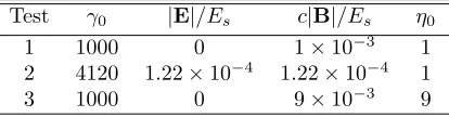
In this section the Monte-Carlo algorithm will be tested in two field config-urations discussed in section 2.3: a constant magnetic field and a circularly po-larised electromagnetic wave. We consider an electron bunch where the electrons initially all have energyγ0mec2, moving perpendicular to the electromagnetic

fields (and counter-propagating relative to the wave in the second configura-tion). The field strengths and values ofγ0for each test case are given in table 1. In each case we compare Φ−, Φγ & Φ+ obtained from Monte-Carlo simulations to direct numerical solution6

of equations (6) & (7). A comparison is also made to a ‘deterministic’ emission model, where Φ−(γ, t) =δ[γ−γd(t)] andγd(t) is

the solution to the equation of motion (9) and to a classical model whereγd is

calcualted assumingg(η) = 1.

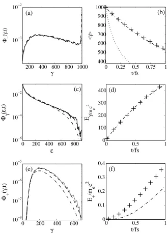
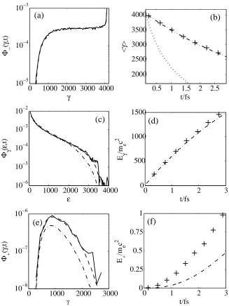
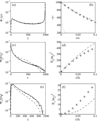
Figures 2 & 3 show results for test problems 1 & 2, where the initialη,η0= 1. The results can be summarised as follows. Φ−, Φγ& Φ+reconstructed from the Monte-Carlo code agree well with those obtained by direct numerical solution of equations (6) & (7). This demonstrates that sufficient particles are used in the Monte-Carlo simulations to adequately sample the energy distributions. Φ−

is extremely broad withσ∼ hγiand soδ[γ−γd(t)] is an extremely poor fit to

the distribution. As a result the deterministic emission model fails to correctly predict the high energy tail in Φγ. The deterministic model does however

cor-rectly determine the total energy radiated as photons and the average electron trajectory. The classical model predicts that the electrons radiate far too much energy. Pair production is sensitive to the high energy tail tail in Φγ and so

the deterministic model fails to predict the total energy emitted as positrons as well as the positron spectrum. The Monte-Carlo algorithm produces the same positron spectrum as the direct solution for Φ+and so also the correct value for the total energy emitted as positrons.

Figure 4 shows the results for test problem 3. In this caseη0= 9. Similarly to test problems 1 & 2 the distributions Φ−, Φγ & Φ+obtained from the Monte-Carlo emission algorithm agree with those from direct solution of equations (6)

6

By first-order upwinding, ensuring the time-step is<10−1

∆tQED.

Test γ0 |E|/Es c|B|/Es η0 1 1000 0 1×10−3

1 2 4120 1.22×10−4

1.22×10−4 1

3 1000 0 9×10−3 ₉

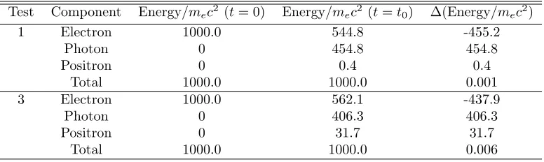
Test Component Energy/mec2(t= 0) Energy/mec2(t=t0) ∆(Energy/mec2)

1 Electron 1000.0 544.8 -455.2

Photon 0 454.8 454.8

Positron 0 0.4 0.4

Total 1000.0 1000.0 0.001

3 Electron 1000.0 562.1 -437.9

Photon 0 406.3 406.3

Positron 0 31.7 31.7

Total 1000.0 1000.0 0.006

Table 2: Energy in each component in Monte-Carlo simulations of test problems 1 (with

Ne= 107) & 3 (withNe= 106). The ‘Total’ in ∆(Energy) refers to the total error in energy conservation summed over all particles in the simulation.

& (7). However, in this case the average electron energy and energy radiated as photons differ from the deterministic model. This is because at such highη

pairs are no longer a minority species and so contribute to the average electron energy and to the radiation of gamma-rays.

4.1. Accuracy, Numerical Convergence & Energy Conservation

To investigate the convergence of the numerical solution, test problem 1 was repeated and the number of macroelectrons (Ne) and the time-step (∆t)

varied. Figures 5(a) & (b) show the decrease in the coefficient of variation

σN/E in the total energy radiated as gamma-ray photons and positrons with

increasingNe. σN/Escales as 1/√Ne. Many more macroelectrons are required

to resolve positron than photon production due to the lower emission rate. Another requirement for obtaining an accurate solution is that ∆t < ∆tQED.

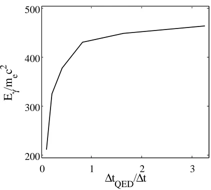
Figure 6 shows how the energy radiated as photons per particle in the Monte-Carlo simulation converges as ∆t is varied between ∆t= 10∆tQED and ∆t =

0.3∆tQED. The error in ǫγ decreases quickly with decreasing time-step; when

∆t = 0.6∆tQED the solution has converged to a reasonable level of accuracy

(3%).

In section 3.1 we demonstrated that the numerical scheme does not conserve energy. Table 2 shows the energy, divided by the initial number of electrons in the bunch, in electrons, photons and positrons at the beginning and end of simulations in the constant B-field test cases (1 & 3), where the electrons & positrons gain no energy from the classical fields. The last column shows the error in energy conservation summed over all particles in the simulation divided byNe. This shows that energy is conserved to a high degree of accuracy

(<0.01%) in each simulation.

5. Discussion

0

200 400 600 800

10

10

10

ε

Φ

(

ε

,t)

0

200

400

600

10

10

10

10

γ

Φ

(

γ

,t)

0

0.5

1

0

100

200

300

400

t/fs

E

0

0.5

1

0

0.1

0.2

0.3

0.4

t/fs

E

/m

c

0

0.25

0.5

0.75

1

400

500

600

700

800

900

1000

t/fs

<

γ

>

200 400 600

800 1000

10

10

γ

Φ

(

γ

,t)

(b)

(a)

(d)

(e)

(f)

(c)

Figure 2: Results for test problem 1: an electron bunch withγ0= 1000 moving perpendicular

to a magnetic field of strengthB= 10−3

Es/c. (a) Φ−(γ, t0 = 1fs) reconstructed from 105

Monte-Carlo trajectories (solid line) compared to the result of direct numerical solution of equation (6) (dashed line). (b)γaveraged over 105

Monte-Carlo trajectories (crosses), the solution for deterministic losses (dot-dashed line) and the classical solution (dotted line). (c) Φγ(γ, t0= 1fs) from the Monte-Carlo simulation (solid line) compared to the result of direct

numerical solution of equation(7) (dashed line) and the spectrum produced by the determin-istic model (dot-dashed line). (d) Total energy radiated as photons from the Monte-Carlo simulation (crosses) and for deterministic emission (dot-dashed line). (e) & (f) Equivalent plots for positrons, where 107

0

1000 2000 3000 4000

10

10

10

γ

Φ

(

γ

,t)

0

1

2

3

0

500

1000

1500

t/fs

E

/m

c

0.5

1

1.5

2

2.5

2000

2500

3000

3500

4000

t/fs

<

γ

>

0

1000 2000 3000 4000

10

10

10

10

10

ε

Φ

(

ε

,t)

0

1000

2000

3000

10

10

10

Φ

(

γ

,t)

0

1

2

3

0

0.5

1

0.25

0.75

t/fs

E

/m

c

(e)

(f)

(d)

(b)

(a)

(c)

Figure 3: Results for test problem 2: an electron bunch withγ0= 4120 counter-propagating

relative to a circularly polarised electromagnetic wave witha= 50. (a) Φ−(γ, t0 = 3fs)

re-constructed from 105

Monte-Carlo trajectories (solid line) compared to the result of direct numerical solution of equation (6) (dashed line). (b)γaveraged over 105

Monte-Carlo trajec-tories (crosses), the solution for deterministic losses (dot-dashed line) and the classical solution (dotted line). (c) Φγ(γ, t0 = 3fs) from the Monte-Carlo simulation (solid line) compared to

the result of direct numerical solution of equation (7) (dashed line) and the spectrum pro-duced by the deterministic model (dot-dashed line). (d) Total energy radiated as photons from the Monte-Carlo simulation (crosses) and the spectrum produced by the deterministic model (dot-dashed line). (e) & (f) Equivalent plots for positrons, where 106

0 500 1000 10−4 10−3 10−2 10−1 ε

Φ

(

ε

,t

)

0 0.05 0.1

0 100 200 300 400 500

t/fs

E

/m

c

0 0.05 0.1

0 5 10 15 20 25 30

t/fs

E

/m

c

0 200 400 600 800 1000

10−6 10−5 10−4 10−3 γ

Φ

(

γ

,t

)

0 500 1000

10−4 10−3 10−2 10−1 γ Φ − ( γ .t)

0 0.05 0.1

200 400 600 800 1000 t/fs < γ >

(c)

(a)

(b)

(e)

(f)

(d)

Figure 4: Results for test problem 3: an electron bunch withγ0= 1000 propagating

perpen-dicular to a magnetic field of strengthB= 9×10−3

Es/c. (a) Φ−(γ, t0= 0.1fs) reconstructed

from 105

Monte-Carlo trajectories (solid line) compared to the result of direct numerical solu-tion of equasolu-tion (6) (dashed-line). (b)γaveraged over 105

Monte-Carlo trajectories (crosses), the solution from the deterministic emission model (dot-dashed line) and the classical solution (dotted line). (c) Φγ(γ, t0= 0.1fs) from the Monte-Carlo simulation (solid line) compared to

10

10

10

10

10

10

10

10

10

N

σ

/

µ

10

10

10

10

10

10

10

N

σ

/

µ

(a)

(b)

Figure 5: (a) Reduction inσN/µfor the total energy radiated as photons in test problem 1 with number of electrons initially present in the simulationNe(crosses) & the 1/√Nescaling (dashed line). (b) The equivalent plot for positrons.

0 1 2 3

200 300 400 500

∆

t

QED

/

∆

t

E

/m

e

c

2

functions were derived for electrons, positrons & photons. It was shown that there is a close correspondence between the moments of these equations and the equation of motion using a deterministic model for the radiation reaction force. Such a deterministic emission model has been adopted by several authors [2, 3, 12]. When the probabilistic QED model and the deterministic model were compared in section 4 it was found that the deterministic model did not correctly predict the emitted photon or positron spectra. Although it was found that in the particular cases considered here the the deterministic model did correctly predict the total energy radiated by the electrons when pair production was negligible7_{. In cases more relevant to experiments, such as a laser pulse striking} a solid target [9, 4] or an electron beam interacting with a laser pulse with a Gaussian temporal envelope, calculations suggest larger differences between the probabilistic & deterministic models. This suggests that the probabilistic Monte-Carlo emission algorithm described here is preferable to a deterministic emission model.

The Monte-Carlo scheme introduces additional numerical constraints on the time-step and the minimum number of macroparticles that can be used in QED-PIC simulations. The time-step must be smaller than ∆tQED. In section 3.1 it

was shown that this only limits the time-step in a QED-PIC simulation of low density plasmas when a > 102

. The total energy emitted as photons & pairs converges with number of macroelectrons in the simulation (Ne) as σN/E =

(1/√Ne)σ/E. The number of macroelectrons required for σN/E to converge

to an acceptable level depends onσ/E which depends on the rate of emission. If the rate of emission is reducedσ/E is increased. This explains why it was found that many more macroparticles were required to get a reasonable degree of convergence in positron emission than in photon emission forη0= 1, as the rate of positron production is considerable lower than that for photon production at this η. However, this is precisely the case when pair production does not affect the plasma dynamics. For η0 = 9, as examined in figure 4, the rate of pair production is higher, pair production does affect the plasma dynamics and in this case the same number of macroparticles is required to resolve positron emission as photon emission.

The emission model breaks down when the fields can no longer be considered as quasi-static or when the laser’s electric field becomes close to the Schwinger field. The former condition is typically only satisfied in situations where emission is unimportant and the latter requires laser pulses of extremely high intensity (1028

Wcm−2

) unlikely to be reached in the near term. We therefore conclude that the emission model outlined here is applicable to a very wide range of laser intensities.

Finally, we note that processes not included in the model might be impor-tant under special conditions. For example, when the rate of pair production is very small, it is dominated by the second-order (inαf) trident process. A

com-7

prehensive discussion of higher order processes can be found in Ref. [33]. Also, in addition to the Coulomb collisions between electrons and ions in the plasma usually included in PIC simulations, additional collisional processes could play role. For example one could include collisions between: gamma-ray photons and electrons/positrons (Compton scattering); electrons and positrons (anni-hilation); electrons/positrons and ions/atoms (bremsstrahlung or Trident pair production in the electric fields of the nuclei); gamma-ray photons and atoms (Bethe-Heitler pair production). A full investigation of the relative importance of these effects is beyond the scope of this paper.

6. Conclusions

When laser pulses of intensity>1021_Wcm−2 _{interact with ultra-relativistic} electrons a significant amount of the electron’s energy is converted to gamma-ray photons & pairs. We have shown that a probabilistic Monte-Carlo algorithm best simulates the emission and that such an algorithm can be coupled to a PIC code to simulate QED-plasmas. By contrast a deterministic treatment of the emission processes only correctly describes the evolution of the particle spectra when pair production can be neglected and so is only valid over a relatively narrow range of laser intensities. We therefore conclude that QED-PIC codes, using the Monte-Carlo emission algorithm described here, will provide a valuable tool for simulating high intensity laser-plasma interactions at today’s highest intensities and beyond.

Acknowledgements

This work was funded by the UK Engineering and Physical Sciences Research Council (EP/G055165/1 & EP/G054940/1). We would like to thank Brian Reville & Alexander Thomas for many useful discussions.

Appendix A. Classical & Quantum Synchtrotron Emissivity

The quantum synchrotron function is given by Sokolov and Ternov [15] eq. (6.5). In our notation it is, forχ < η/2

F(η, χ) = 4χ 2

η2 yK2/3(y) +

1−2_ηχ

y

Z ∞

y

dt K5/3(t) (A.1)

wherey= 4χ/[3η(η−2χ)] &Kn are modified Bessel functions of the second

kind. Forχ≥η/2,F(η, χ) = 0.

In the classical limit~ _{→0 the quantum synchrotron spectrum reduces to}

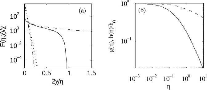
the classical synchrotron spectrumF(η, χ) →ycR_y∞c duK5/3(u); yc = 4χ/3η 2_. For comparison the classical and quantum synchrotron spectra are plotted for

0 0.5 1 1.5 10−4

10−2 100 102

2χ/η

F(

η

,

χ

)/

χ

10−3 10−2 10−1 100 101 10−1

100

η

g(

η

), h(

η

)/h

0

(a) (b)

Figure A.7: (a)F(η, χ)/χand the equivalent classical spectrum plotted forη= 0.01 (dash-dot and dotted lines respectively) &η= 1 (solid and dashed lines respectively). (b)g(η) (solid line) &h(η) (dashed line).

As stated in section 2.1, the modification to the spectrum leads to a reduction in the radiated power by a factorg(η), where a fit to this function was given. The photon emissivity is also reduced by a factor ofh(η)/h0. g(η) & h(η) are expressed in terms ofF(η, χ) as

g(η) = 3 √

3 2πη2

Z η/2

0

dχF(η, χ) h(η) =

Z η/2

0

dχF(η, χ)

χ (A.2)

These functions are plotted in figure A.7(b). Hereh(η) has been normalised to the classical value h0 = 5.24. Quantum corrections to the photon emission become important wheng(η) andh(η)/h0 deviate from unity.

Appendix B. Pair Emissivity

The approximate form of the function controlling the rate of pair production used here is [14]

T±≈0.16

K2

1/3[2/(3χ)]

χ (B.1)

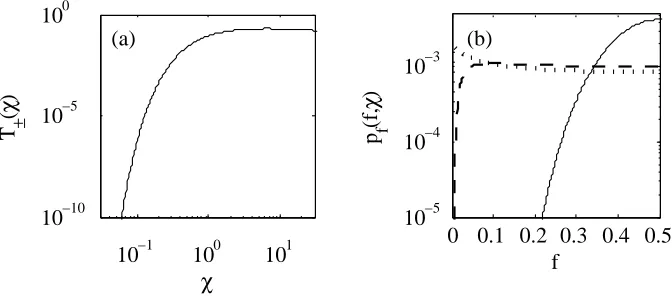
This function is plotted in figure B.8(a). Note the extremely rapid increase withχ; for lowχ T±(χ)∝exp[−2/(3χ)]. For highχ T±(χ) falls off asχ−1/3.

The function controlling the distribution of the photon energy between the electron and positron in the pair,pf(f, χ), is given by [30]

pf(f, χ) =

2 +f(1−f)

f(1−f) K2/3

₁

3χf(1−f)

₁

0 0.1 0.2 0.3 0.4 0.5

10

10

10

f

p

(f,

χ

)

10

10

10

10

10

10

χ

T

(

χ

)

(a)

(b)

Figure B.8: . (a)T±(χ). (b)pf(f, χ) plotted forχ= 0.1 (solid line)χ= 10 (dashed line) &

χ= 100 (dotted line).

Where k(χ) is a normalisation constant such thatR1

0 df pf(f, χ) = 1. Note thatpf(f, χ) =pf(1−f, χ) and so is symmetrical inf aboutf = 0.5.

In the limitsχ≪1 &χ≫1 pf approaches

pf(f, χ)≈

2 +f(1−f) (χf(1−f))1/2exp

− 1

3χf(1−f)

₁

k(χ) χ≪1 (B.3)

pf(f, χ)≈ 2 +f(1−f)

(χf(1−f))1/3 1

k(χ) χ≫ 1

f(1−f) (B.4)

Therefore, pf(f, χ) is sharply peaked at f = 0.5 for χ ≪ 1 and peaked at

f ≈0 &f ≈1 forχ≫1. This is demonstrated by figure B.8(b), wherepf(f, χ)

is plotted forχ= 0.1,1 & 100.

References

[1] P. A. M. Dirac, Proc. R. Soc. A,167, 148 (1938)

[2] J.G. Kirk, A.R. Bell & I. Arka, Plas. Phys. Control Fusion, 51, 085008 (2009)

[3] I.V. Sokolovet al, Phys. Rev. E,81, 036412 (2010)

[4] R. Duclous, J.G. Kirk & A.R. Bell, Plas. Phys. Control Fusion,53, 015009 (2011)

[5] N.V. Elkinaet al, Phys. Rev. ST. AB.,14, 054401 (2011)

[6] A.R. Bell & J.G. Kirk, Phys. Rev. Lett.,101, 200403 (2008); A.M. Fedotov

[7] E.N. Nerushet al, Phys. Rev. Lett.,106, 035001 (2011)

[8] I.V. Sokolov, N.M. Naumova & J.A. Nees, Phys. Plasmas, 18, 093109 (2011)

[9] C.P. Ridgerset al, Phys. Rev. Lett.,108, 165006 (2012); C.S. Brady et al, Phys. Rev. Lett.,109, 245006 (2012)

[10] P. Goldreich, & W.H. Julian, Astrophys. J.,157, 869 (1969); R.D. Bland-ford, & R.L. Znajek, Mon. Not. R. Astron. Soc.,179, 433 (1977)

[11] J.M. Dawson, Phys. Fluids,5, 445 (1962); C.K. Birdsall & A.B. Langdon, Plasma physics via computer simulation (McGraw-Hill, New York, 1985)

[12] A. Zhidkovet al, Phys. Rev. Lett.,88, 185002 (2002); S. Kiselev, A. Pukhov & I. Kostyukov, Phys. Rev. Lett93, 135004 (2003); N. Naumovaet al, Eur. Phys. J. D,55, 393 (2009); M. Tamburiniet al, New J. Phys.,12, 123005 (2010); M. Chen et al, Plasma Phys. Control. Fusion, 53, 014004 (2011); T. Nakamuraet al, Phys. Rev. Lett.,108, 195001 (2012)

[13] F. Sauter, Z. Phys.69, 742 (1931); W. Heisenberg & H. Euler, Z. Phys.

98, 714 (1936); J. Schwinger, Phys. Rev.,82, 664 (1951)

[14] T. Erber, Rev. Mod. Phys.,38, 626 (1966)

[15] A.A. Sokolov & I.M. Ternov, ’Synchorotron Radiation’, Akademie-Verlag, Berlin, 1968

[16] C.S.Shen & D. White, Phys. Rev. Lett.,28, 455 (1972)

[17] W.P. Leemanset al, Nature Phys., 2, 696 (2006); S. Karschet al, New J. Phys.,9, 415 (2007); N.A.M. Hafzet al, Nature Photonics,2, 571 (2008)

[18] I.V. Sokolov,et al, Phys. Rev. Lett.,105, 195005 (2010)

[19] A.G.R. Thomas, C.P. Ridgers, S.S. Bulanov, B.J. Griffin & S.P.D. Mangles, Phys. Rev. X,2, 041004 (2012)

[20] K.K. Andersenet al, Phys. Rev. D,86, 072001 (2012)

[21] C. Bulaet al, Phys. Rev. Lett., 76, 3116 (1996); D.L. Burke et al, Phys. Rev. Lett.,79, 1626 (1997)

[22] K. Ta Phouc, Nature Photonics,6, 308 (2012)

[23] H. Chenet al, Phys. Rev. Lett.,105, 15003 (2010)

[24] G.A. Mourouet al, Plasma Phys. Control. Fusion,49, B667 (2007)

[25] A.N. Timhokin, Mon. Not. R. Astron. Soc.,408, 2092 (2010)

[27] V.N. Baier & V.M. Katkov, Sov. Phys. JETP,26, 854 (1968)

[28] W.H. Furry, Phys. Rev.,81, 115 (1951)

[29] V.I. Ritus, J. Russ. Laser Res.,6, 497 (1985)

[30] J.K. Daugherty & A.K. Harding, Astrophys. J.,273, 761 (1983)

[31] A. DiPiazza, K.Z. Hatsagortsyan & C.H. Keitel, Phys. Rev. Lett., 105, 220403 (2010)

[32] L. D. Landau and E. M. Lifshitz, The Course of Theoretical Physics (Butterworth-Heinemann, Oxford, 1987), Vol. 2., p222-225