Expectations and the saving behaviour of children: analysis of the U.S. panel study of income dynamics

(1)

This is a repository copy of Expectations and the saving behaviour of children: analysis of the U.S. panel study of income dynamics.

White Rose Research Online URL for this paper: http://eprints.whiterose.ac.uk/74396/

Monograph:

Brown, S. and Taylor, K. (2012) Expectations and the saving behaviour of children: analysis of the U.S. panel study of income dynamics. Working Paper. Department of Economics, University of Sheffield ISSN 1749-8368

2012015

[email protected] https://eprints.whiterose.ac.uk/ Reuse

Unless indicated otherwise, fulltext items are protected by copyright with all rights reserved. The copyright exception in section 29 of the Copyright, Designs and Patents Act 1988 allows the making of a single copy solely for the purpose of non-commercial research or private study within the limits of fair dealing. The publisher or other rights-holder may allow further reproduction and re-use of this version - refer to the White Rose Research Online record for this item. Where records identify the publisher as the copyright holder, users can verify any specific terms of use on the publisher’s website.

Takedown

If you consider content in White Rose Research Online to be in breach of UK law, please notify us by

(2)

Sheffield Economic Research Paper Series

SERP Number: 2012015

ISSN 1749-8368

Sarah Brown

Karl Taylor

Expectations and the Saving Behaviour of Children: Analysis of the U.S.

Panel Study of Income Dynamics

June 2012

Department of Economics University of Sheffield 9 Mappin Street Sheffield S1 4DT

United Kingdom

(3)

Expectations and the Saving Behaviour of Children:

Analysis of the U.S. Panel Study of Income Dynamics

Sarah Brown and Karl Taylor

Department of Economics University of Sheffield

9 Mappin Street Sheffield S1 4DT

United Kingdom

Abstract: In this paper, we analyse the saving behaviour of a sample of children

drawn from the 2002 and 2007 Child Development Supplements of the U.S. Panel

Study of Income Dynamics. In particular, we focus on the influence of children’s

expectations and attitudes towards the future on the total level of children’s savings as well as on savings specifically for future education and savings for other purposes. Overall, our findings suggest that the saving behaviour of children, as measured by the level of savings, appears to be influenced by their expectations, especially expectations regarding future educational attainment and life expectancy. Specifically, the level of savings held by children is monotonically increasing in the expected level of educational attainment and children who are pessimistic about their future life expectancy are found to hold lower levels of savings, which is consistent with discounting future consumption heavily.

Key Words: Expectations; Household Finances; Intergenerational Analysis; Saving.

JEL Classification: D12; D14

Acknowledgements: We are grateful to the Institute for Social Research, University

of Michigan for supplying the Panel Study of Income Dynamics 2001 to 2007. We are especially grateful to Jennifer Roberts and Anita Ratcliffe for excellent comments and advice. The normal disclaimer applies.

(4)

2

1. Introduction and Background

In the aftermath of the recent financial crisis, there has been increasing interest in the

financial literacy of young adults and in the role of financial education in preparing

children and young adults for entry into a complex economic and financial

environment. Evidence has suggested that the financial literacy of children and young

adults is somewhat lacking. For example, Lusardi et al. (2008) find that only 27% of

young individuals in their sample drawn from the U.S. National Longitudinal Survey

of Youth were knowledgeable about basic financial concepts. Hence, it is perhaps not

surprising that a number of individuals encounter financial problems during

adulthood: Garon (2012), p. 1, comments that, in the U.S., ‘it has become painfully

clear that millions lack the savings to protect themselves against foreclosures,

unemployment, medical emergencies, and impoverished retirements.’ Hence, the

general consensus amongst academics and policy-makers is that we are not saving

enough, especially in the context of saving for retirement, yet research into how

attitudes towards saving are influenced at an early stage of the life cycle is relatively

scarce.

From a policy perspective, in the U.S., there has been evidence reported in

support of financial education programmes as a means to enhance financial outcomes.

For example, Bernheim et al. (2001) explore the effect of high school financial

curriculum mandates, which were adopted by some U.S. states, on asset accumulation

and saving during adulthood. Such mandates were found to increase exposure to

financial education. Moreover, asset accumulation and saving were found to be higher

amongst individuals who received such education. In addition, the findings indicated

a positive relationship between the amount saved during adulthood and having saved

(5)

3

require financial education at high school: for example, Cole and Shastry (2009)

report that 28 U.S. states have mandatory financial literacy programmes at high

school. However, their findings, which are based on a different data set and

instrumental variable strategy to that of Bernheim et al. (2001), indicate that some

U.S. state mandated financial literacy programmes did not influence saving

behaviour, suggesting that the role of such programmes may be less clear-cut. Despite

such evidence, there has been increasing support for formal financial education at

elementary school, see, for example, Sherraden et al., 2011, who explore a four year

elementary school based programme, ‘I Can Save’, where those children who

participated in the programme attained higher scores in a fourth grade financial

literacy test than those in the control group.1

It is apparent that children and young adults may acquire financial literacy

skills from their parents as well as from school and formal education. For example,

Mandell (2007) reports that parents are the key source of financial information for

students at high school. Such findings tie in with the recent education literature

exploring the relationship between the educational attainment of parents and their

children (see Black and Devereux, 2011, for a recent survey), where extensive

empirical evidence has supported the existence of a strong positive intergenerational

association in educational attainment, which clearly has implications for future

income and wealth generation.2 A related strand of the literature on intergenerational

aspects of economic and financial attitudes has focused on estimating the

1_{There has also been recent interest amongst policy-makers in the U.K. in promoting financial literacy}

amongst children and adults to enhance financial outcomes. For example, ‘Economic Well-being and Financial Capability’ forms part of the U.K. National Curriculum for schools, albeit a non-statutory component, with the aim of teaching school pupils to manage their money and finances effectively. Guidance on how to incorporate personal finance education into the curriculum is provided nationally by the Department for Education.

2

(6)

4

intergenerational elasticity of wealth between parents and their adult children. For

example, Charles and Hurst (2003) estimate this elasticity at 0.37 for the U.S. using

data from the Panel Study of Income Dynamics (PSID), whilst Arrondel (2009)

reports an estimate of 0.22 for France. Thus, the findings in the existing literature

support a sizeable intergenerational correlation of wealth.

Despite such increasing interest in financial literacy, financial outcomes and

financial education programmes, research on the saving behaviour and the financial

decision-making of children and young adults remains relatively scarce, especially in

the economics literature. Furthermore, as Elliott et al. (2011), p. 1101, comment

‘research and policy on savings often overlooks children as agents, capable of saving.’

Although, as Crossley et al. (2012) argue, children are unlikely to hold significant

financial assets or to be faced with any ‘substantive financial decisions’, it is apparent

that they may be faced with decisions on a smaller scale such as whether to save for a

toy or the latest mobile phone and such decision-making may shape their attitudes

towards finances in the future. In addition, the rising consumption of children and

young adults has started to attract the attention of researchers leading to more focus

on this increasingly important aspect of household financial decision-making

(Sherraden et al., 2011).

There is growing interest in this area from a range of disciplines including

economics, education and psychology and sociology. For example, using U.S. data,

Knowles and Postlewaite (2004) find that parents’ saving behaviour influences the

saving behaviour of their adult offspring. Similarly, Cronqvist and Siegel (2010),

using data on Swedish twins aged between 18 and 65, explore the origins of saving

behaviour. Their findings suggest that an individual’s propensity to save is influenced

(7)

5

parent to offspring transmission in saving behaviour is found to be important for

young individuals. There has also been some interest in the saving behaviour of young

children in the economic psychology literature. For example, Otto et al. (2006)

explore children’s use of saving strategies in the context of saving for a toy when

faced with income uncertainty. The results indicated that children aged between 9 and

12 are able to formally manage their money, with children aged 12 frequently making

‘bank’ deposits as a means to avoid the temptation to spend tokens on, for example,

sweets.

We contribute to the existing literature on household finances by exploring the

saving behaviour of children. In particular, we focus on the influence of children’s

expectations and attitudes towards the future on their saving behaviour. Although

individuals’ expectations play a central role in economic theory, microeconometric

evidence of their causes and effects is, somewhat surprisingly, relatively sparse. The

work that does exist is predominately focused on adults’ financial expectations,

exploring the motivation behind, for example, debt accumulation, spending, saving

and investment (see, for example, Brown et al., 2005, 2008, Das and van Soest, 1999

and Souleles, 2004). Hence, we expand this literature by analysing the influence of

the expectations of children on their saving behaviour, thereby bringing together two

relatively unexplored areas of the economics literature. Overall, our findings suggest

that the saving behaviour of children, as measured by the level of savings, appears to

be influenced by their expectations, especially in the case of expectations regarding

future educational attainment and life expectancy. Specifically, the level of savings

held by children is monotonically increasing in the expected level of educational

(8)

6

found to hold lower levels of savings, which is consistent with heavy discounting of

future consumption.

2. Data and Methodology

We analyse data drawn from the U.S. Panel Study of Income Dynamics (PSID), which

is a panel of households ongoing since 1968 conducted at the Institute for Social

Research, University of Michigan. We focus on data from the 2002 and 2007 Child

Development Supplements (CDS), which provide additional information relating to

parents in the PSID and their children, with the objective being to provide information

on early human capital formation. We match the information in the CDS with that

available in the main head of family PSID questionnaires for 2001 and 2007, which

provide information on household characteristics.3 Our sample comprises 2,646

observations.

With respect to information on the saving behaviour of children, children aged

12 to 17 were asked: Do you have a savings or bank account in your name? Those

that responded that they had such an account were asked to specify how much was in

the account. The responses thus provide information relating to the stock of savings

held by the children at that point in time. The children were also asked the following:

are you saving some of this money for future schooling, like college?; how much have

you saved for future schooling?; and are you saving this money for something besides

school? Hence, we distinguish between three different types of saving in our

empirical analysis: the amount of total saving (ts_it) of child i at time t; the amount

saved for educational purposes (es_it) of child i at time t; and the total amount saved

for non educational purposes (os_it) of child i at time t.

(9)

7

We are also able to construct a proxy for the flow of saving since information

on the total income (y_it) and expenditure of the child (e_it) is available, the proxy for

the flow of saving being defined as the difference between these two measures,

it it it

sf = y −e . The weekly income received by children is the sum of that received

from parental allowances or pocket money and income earned from part-time work.

With respect to the expenditure of child i at time t, e_it, we focus on total expenditure

per week on: music, games, clothes, books, going out, cars, public transport, hobbies

and gifts.

As stated above, we focus on the relationship between children’s expectations

and attitudes towards the future and their saving behaviour. The CDS provides

information on expectations and attitudes relating to a range of areas, which we

exploit in order to compare the influences of expectations regarding different aspects

of the child’s life. Specifically, we analyse educational expectations as discerned from

the child’s responses to the following question: Many people do not get as much

education as they would like. How far do you think you will actually go in school? Do

you think you will: leave high school before graduation; graduate from high school;

graduate from a two-year community college; graduate from a vocational school;

attend a four-year college; graduate from a four-year college; or get more than four

years of college. We also analyse the influence of the frequency at which the child

worries that they will not get a good job when they are an adult and the frequency at

which the child feels discouraged about the future, distinguishing between: 1 to 3

times a week; and almost daily/every day. We also explore the influence of the child

believing that there is ‘no chance’ that they will have enough money to support

(10)

8

extent to which the child may discount the future, we analyse the influence of the

child believing that they will not live past the age of 21.

To analyse the relationship between expectations and children’s saving

behaviour, we treat ts_it, es_it, and os_it as censored dependent variables in our

econometric analysis since they cannot have negative values. For total savings, ts_it,

approximately 62.6% of children hold no savings. With respect to savings for future

education (es_it) and for other reasons (os_it), the percentages who hold no savings are

77.4% and 76.9%, respectively. Figure 1 shows the distribution of the natural

logarithm of total savings, for those children who hold savings, and also for savings

for educational purposes and for other reasons. Following Bertaut and Starr-McCluer

(2002), we employ a censored regression approach to ascertain the determinants of

( )

ln tsit , ln

( )

esit and ln

( )

osit , which allows for the truncation of the dependent

variables.4 As the distributions of the dependent variables are highly skewed,

following Gropp et al. (1997), we specify logarithmic dependent variables. We denote

by

( )

*

ln tsit ,

( )

*

ln esit and

( )

*

ln osit the corresponding untruncated latent variables,

which theoretically can have negative values.

We model each dependent variable via a random effects tobit specification, as

shown below for ln

( )

tsit :

( )

*

ln ts_it =β′X_it+γExp_it+ =ν_it θθθθ′Z_it+ν_it (1)

( )

ln ts_it = ln ts*_it if ln ts*_it >0 (2)

( )

ln ts_it =0 otherwise (3)

(11)

9

where the total savings of child i at time t are given by ts_it such that i=1,…,n and

t=1,…,T, X_it denotes a vector of child and household characteristics, Exp_it denotes

the measure of expectations and ν_it is the stochastic disturbance term. The structure

of the error terms is given as follows: ν_it = +α η_i _it, where α_i is an individual specific

unobservable effect, and η_it is a random error term, η ∼_it IID

( )

0,σ_it2 .

Figure 2 shows the distribution of sf , where approximately 54% of _it

observations of sf_it =y_it−e_it are negative, i.e. where weekly expenditure exceeds

weekly income indicating a gap between income and consumption behaviour, which

may be met by transfers from parents or other relatives given that children cannot

enter into formal credit arrangements. In order to explore the determinants of ln

( )

sf_it ,

we conduct quantile analysis given the continuous nature of the dependent variable

(see Koenker and Bassett Jr., 1978), where ln

( )

sf_it =ln

(

y_it−e_it

)

if

(

y_it−e_it

)

>0;

( )

(

)

ln sf_it = −1 ln y_it−e_it if

(

y_it −e_it

)

<0, otherwise ln

( )

sf_it is set to zero since

there are no values of

(

y_it−e_it

)

between zero and unity. As stated by Brown and

Taylor (2008), the advantage of quantile regression analysis over regression at the

mean (i.e. OLS) is that it provides an analysis of different parts of the conditional

distribution hence providing a fuller description of the entire distribution. This is

because when considering the effect of an explanatory variable on the dependent

variable, under quantile regression analysis, the effect is allowed to vary at different

quantiles of the conditional distribution. Thus, instead of assuming that covariates

shift only the location or the scale of the conditional distribution, quantile regression

explores the potential effects of covariates on the shape of the distribution. Hence,

(12)

10

mean, may have a statistically significant role at certain parts of the saving

distribution or may differ in terms of the magnitude of the effect, Koenker and

Hallock (2001). The quantile regression approach is given by:

( )

ln sfit =ππππθ′Xit+φθExpit+εθit, (4)

where ε_θ_it is the error term associated with the θth quantile of ln

( )

sfit and

(

it it, it

)

0

Quant_θ ε_θ X Exp = . The θth conditional quantile of ln

( )

sfit for a given set of

characteristics, Xit and expectations, Expit, is denoted by:

( )

{

ln sit it, it

}

it it

Quant_θ f X Exp =ππππ_θ′X +φ_θExp , (5)

where ππππ_θ and φ_θ denote vectors of parameters. We explore each percentile of the

distribution in order to investigate whether the influence of expectations is uniform

across the distribution.

In terms of the explanatory variables included in the tobit and quantile

analyses, we control for characteristics of the child including: gender; ethnicity; and

age. We also control for the number of books that the child has as well as the

children’s standardized scores in the widely used Woodcock-Johnson Revised

Achievement Tests, namely, the applied problems test, the letter word identification

test and the passage comprehension test.5 In the tobit analysis, we control for the

child’s weekly allowance which is related to chores ‘like yard work or cleaning the

house’, the child’s weekly allowance which is unrelated to chores6 and the weekly pay

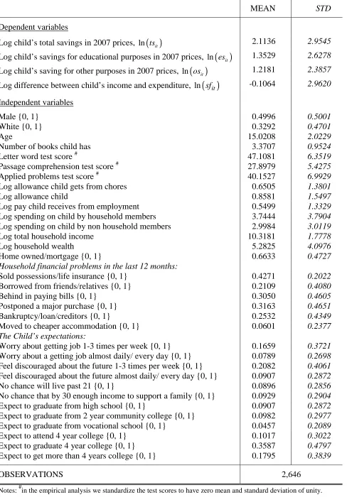
5_{These tests have been validated extensively (see Woodcock and Johnson, 1990, for further details of}

the tests). Each academic test score is standardized, i.e. normalised to have zero mean and standard deviation of unity.

6

(13)

11

received by the child for part-time work.7 In order to control for other financial

transfers received by the child, we control for total annual spending on the child by

household members as well as such expenditure by non household members. In terms

of household characteristics, we control for: annual total household income;

household wealth; and whether the house is owned outright or via a mortgage. We

also control for whether the household has done any of the following or has had any

of the following happen as a result of economic problems over the last 12 months:

sold possessions or cashed in life insurance; postponed major purchases or medical

care; borrowed money from friends or relatives; fallen behind in paying bills; filed for

or taken bankruptcy, had a creditor call or visit to demand payment, had wages

attached or garnisheed by a creditor, had a lien filed against the property as a bill

could not be paid or had the home, car or other property repossessed; or moved to

cheaper accommodation. Finally, we include state controls to allow for regional

differences in the provision of financial education in schools. Summary statistics

related to all of the variables used in our econometric analysis are presented in Table

A1 in the appendix.

3. Results

Random Effects Tobit Analysis of Saving

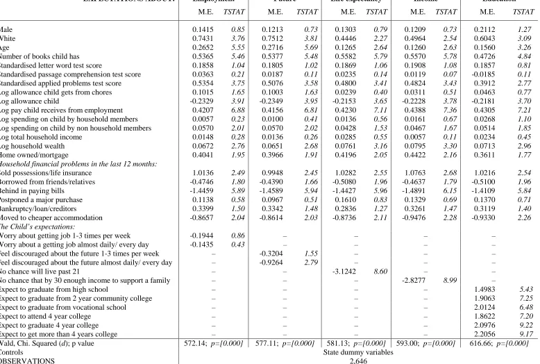
The results relating to the random effects tobit analysis of the determinants of the

level of total savings of the child are presented in Table 1, where each column

controls for a different type of expectation, namely expectations regarding

employment, the future, life expectancy, income and education. Marginal effects are

children may provide to parents such as carrying out household chores and preference shaping relates to the provision of economic education.

7_{A small number of studies have explored the relationship between parental allowances and children’s}

(14)

12

presented throughout and are derived from the derivative of the conditional expected

value of the truncated logged response, given the covariates, with respect to the

covariates, Z . The conditional expected value function of the truncated logged _it

response, such as ln

( )

ts_it from equation (1), is given by the following

( )

{

ln _it _it

}

(

' _it

)

' _it

{

(

' _it

)

}

E ts Z = Φ θθθθ Z //// σ θθθθ Z +σ φ θθθθ Z //// σ (and will be heavily

weighted towards zero), where φ and Φ denote the density and cumulative

distribution of the standard normal. The standard error of the regression is given by σ.

Differentiation of the expected value function with respect to Z , the _kit kth covariate,

gives: ∂E

{

ln

( )

ts_it Z_it

}

/∂Z_kit = Φ

(

θθθθ'Z_it /σ θ

)

_k = prob

{

ln

( )

ts_it >0 Z_it

}

θ_k. The

probability of having a positive outcome can be approximated by the scaling factor,

i.e. the proportion of uncensored observations of the dependent variable. The marginal

effects reported in Tables 1 and 2 are found by multiplying the estimated coefficients

through by the relevant scaling factor.

It is apparent that concerns regarding getting a job in adulthood do not appear

to influence the amount of savings held by the child. In contrast, if the child feels

discouraged about the future almost daily or every day is inversely associated with the

level of savings. Such feelings may lead to the child discounting the future heavily

with less concern for saving. In a similar vein, there is a very large and highly

statistically significant inverse effect on the level of saving if the child believes that

there is no chance that he/she will live beyond 21. Such findings are consistent with

focusing on current consumption rather than saving for the future. However, if the

child believes that there is no chance that they will earn enough income by the age of

30 to support a family is also characterised by a relatively large and statistically

(15)

13

reflects current financial difficulties or constraints faced by the child and, hence, a

low balance in their bank account. With respect to educational expectations, it is clear

that expectations about all levels of education are positively related to the level of

savings relative to expecting to leave high school before graduation. Furthermore,

with the exception of the category relating to expecting to attend a four year college, it

is apparent that the estimated effects are monotonically increasing in expectation of

attaining a higher level of education.8,9

Given that the focus of our analysis is on the role of expectations, we

comment only briefly on the results relating to the other explanatory variables, which

have consistent effects across the five specifications. Gender does not appear to

influence the amount of saving whereas age and being white are both positively

associated with the amount of saving. It is interesting to see that the applied problems

test score, which reflects aptitude in mathematics, is positively associated with the

level of savings whilst the letter-word and passage comprehension tests both have

statistically insignificant influences.

The importance of distinguishing between the sources of income of the

children is apparent with income associated with part-time work having a positive

8

It may be the case that the child’s expectations about their future educational attainment are picking up the aspirations of their parents. In the 2002 and 2007 CDS, information is provided by the primary care giver on what they hope their child will achieve, specifically they are asked: In the best of all

worlds, how much schooling would you like the child to complete? The response categories to this

question closely mirror those provided by the child (see Section 2). We have also estimated specifications including binary indicators for the parent’s aspirations about their child’s educational attainment as well as incorporating the child’s own expectations regarding their future schooling. Interestingly, for each type of saving, only the educational expectations of the child matter with the aspirations of the parent always being jointly statistically insignificant at the 5 per cent level.

9_{We have also investigated whether children’s expectations still matter when we control for parental}

(16)

14

influence on the amount of savings, the amount of the allowance that is unrelated to

chores having a negative influence and the amount of the allowance associated with

chores being characterised by a statistically insignificant influence. The influence of

the allowance that is unrelated to chores may be similar to a windfall effect

characterised by a large marginal propensity to consume from this additional

unearned income. For example, Imbens et al. (2001), who analyse a sample of U.S.

lottery players, find that recent winners are estimated to have lower savings rates than

individuals who won the lottery some time ago and that non-winners save more in

retirement accounts than winners.

With respect to household characteristics, household wealth is positively

related to the level of savings. Some of the controls for the existence of household

financial problems exert negative influences on the child’s level of savings, with the

exception of having sold possessions or life insurance which exerts a relatively large

positive influence. It may be the case that this positive influence reflects the fact that

the household was able to afford such purchases in the past or, alternatively, the

money raised may have been transferred to the child.

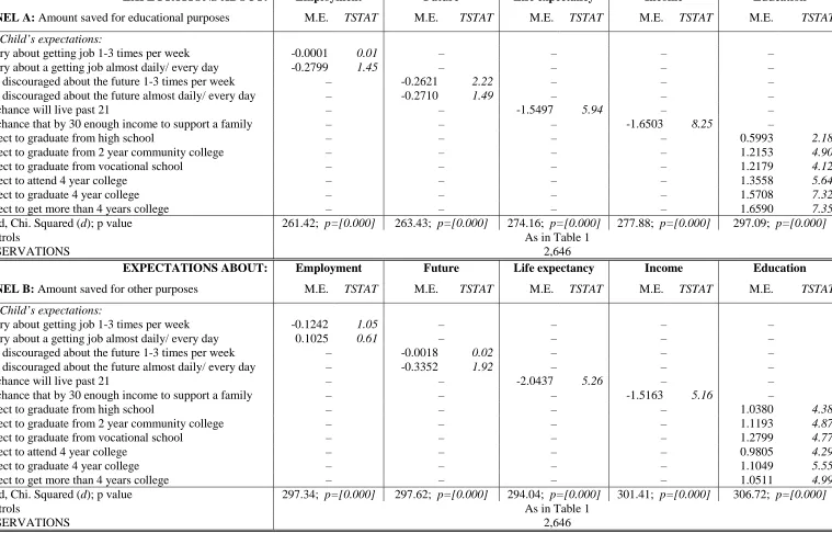
For brevity, in Table 2, where we decompose the total saving of the child into

savings for education (Panel A) and savings for other purposes (Panel B), we only

present the results related to the expectations variables. It is apparent that the pattern

of the results in Table 2 Panel A is generally in line with that presented in Table 1,

albeit with the magnitudes of the effects being somewhat larger. This is especially

apparent in the case of the inverse effect associated with the child believing that they

have no chance of living beyond the age of 21. The effects associated with

educational expectations are also heightened relative to those in Table 1, with the

(17)

15

level of educational attainment.10 In Table 2 Panel B, the results follow the same

pattern albeit with larger effects estimated in the cases of income expectations in

adulthood and educational expectations relative to those presented in Table 2 Panel

A.11

Overall, our findings suggest that the saving behaviour of children, as

measured by the level of savings, appears to be influenced by their expectations,

especially in the case of expectations regarding future educational attainment and life

expectancy. Finally, if all of the expectations variables are entered simultaneously

then only the child’s expectations about educational attainment and life expectancy

are statistically significant, where the marginal effect of the latter dominates in terms

of magnitude.

Quantile Analysis of the Difference between Income and Expenditure

Tables 3A to 3C summarise the results from the quantile analysis presenting the

effects of the five types of expectations on each percentile of the distribution of our

proxy for the flow of saving, sf_it = y_it−e_it. Negative values for the average difference

between income and expenditure exist across the 10th to the 50th deciles, with this part

of the distribution being characterised by expenditure in excess of income.

In Table 3A, it is apparent that having concerns regarding future employment

almost every day or daily is inversely associated with the two lowest deciles of the

distribution of the gap between income and expenditure, where the extent to which

expenditure exceeds income is at its largest. Such concerns, hence, appear to lower

the extent to which the child tends to consume beyond their income, whereas concerns

10_{In the 2002 and 2007 CDS, the primary care giver is asked: Other than what you told me about} already, do you have money set aside for the child to attend college or other future schooling? If

included as an additional control, the natural logarithm of this variable has a positive and statistically significant association with the child’s total savings and savings towards education, having the largest influence on the latter, but is unrelated to the child’s savings for other purposes.

11

(18)

16

regarding the future more generally do not appear to influence the difference between

the children’s income and expenditure.

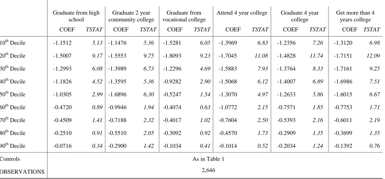
Turning to Table 3B, it is apparent that educational expectations generally

have large and highly statistically significant inverse effects across the 10th to 50th

deciles of the distribution of the gap between income and expenditure, namely, those

parts of the distribution characterised by consumption in excess of income. Beyond

the 50th decile, the effects of educational expectations generally fail to attain statistical

significance. Our findings, thus, suggest that having educational expectations

pertaining to any level of education, which exceeds leaving high school prior to

graduation, is strongly inversely associated with levels of consumption in excess of

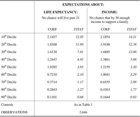
income.12 In contrast, the results summarised in Table 3C indicate that if the child

believes there is no chance that they will live past 21 has a large and highly

statistically significant influence on the 10th to 50th deciles of the distribution of our

proxy for the flow of savings suggesting that such expectations are positively related

to consumption in excess of income which accords with discounting the future

heavily. Similarly, if the child believes there is no chance that he/she will have

enough income by the age of 30 to support their family is positively associated with

the 10th to 50th deciles of the distribution of the gap between income and

consumption, which is associated with the part of distribution where consumption

exceeds income. It is also apparent that positive and statistically significant influences

are also found at the 60th and 70th deciles, although the positive influence is

monotonically decreasing in terms of magnitude moving towards the 90th decile.

Hence, the findings from the quantile analysis endorse the findings from the

tobit analysis in that children’s expectations about and attitudes towards the future,

12_{We have also explored the influence of parental aspirations regarding their child’s educational}

(19)

17

especially those relating to education and life expectancy, are found to be important

influences on their saving behaviour. Our empirical analysis thus provides an insight

into the factors that influence children and young adults in living either within (where

income exceeds consumption) or beyond (where consumption exceeds income) their

means at an early stage of their life.

4. Conclusion

The U.S. economy has been characterised historically by low savings rates. For

example, Garon (2012), page 4, who explores the history of savings promotion in

Europe, the U.S., Japan and other Asian countries, comments, with reference to

savings rates in OECD countries over the period 1985 to 2008, that: ‘by nearly every

measure, the United States jumps out as exceptional in its low saving and

turbocharged consumption.’ Clearly, in the U.S., the focus has historically been

placed on consumption rather than saving as a means to enhance economic growth

with heavy reliance on the expansion of credit. It is apparent, however, that

households with low or no savings but which hold debt are particularly vulnerable to

financial shocks such as redundancy or increases in the cost of living as well as to

changes in their personal lives such as having children or getting divorced. It is

important, therefore, that further research on the saving behaviour of individuals and

households is conducted in order to aid our understanding of this aspect of financial

decision-making. Given the importance of education and human capital acquisition

during childhood, it is apparent that analysing the saving behaviour of children may

be a fruitful line of enquiry. As well as contributing to the existing literature on

household finances by exploring the saving behaviour of children, our analysis also

serves to inform us about the influence of children’s expectations, which, to our

(20)

18

Overall, our findings suggest that the saving behaviour of children, as

measured by the level of savings, appears to be influenced by their expectations,

especially in the case of expectations regarding future educational attainment and life

expectancy. Specifically, the level of savings held by children is monotonically

increasing in the expected level of educational attainment and children who are

pessimistic about their future life expectancy are found to hold lower levels of

savings, which is consistent with discounting future consumption heavily. We find

that such influences are heightened in terms of magnitude in the context of the amount

of savings held specifically for the purposes of future education. Our findings thus

suggest that, as in the case of adulthood, expectations and attitudes towards the future

influence financial decision-making and serve to play an important role in the

accumulation of savings. Given that behaviour in childhood may influence that in

adulthood, our findings offer an insight into the determinants of saving behaviour at

an early stage of the life cycle and hopefully will serve to stimulate future research in

this relatively unexplored area.

References

Arrondel, L. (2009). ‘My Father was Right: The Transmission of Values between

Generations.’ Paris School of Economics Working Paper Number 2009-12.

Barnet-Verzat, C. and F.-C. Wolff (2002). ‘Motives for Pocket Money Allowance and

Family Incentives.’ Journal of Economic Psychology, 23, 339-366.

Bernheim, B. D., Garrett, D. M. and D. M. Maki (2001). ‘Education and Saving: The

Long-Term Effects of High School Financial Curriculum Mandates.’ Journal of

Public Economics, 80, 436-467.

Bertaut, C. and M. Starr-McCluer (2002). ‘Household Portfolios in the U.S.’ In

(21)

19

Black, S. E. and P. J. Devereux (2011). ‘Recent Developments in Intergenerational

Mobility.’ In The Handbook of Labor Economics, O. Ashenfelter and D. Card

(Eds.) Chapter 16, 1487-1541.

Brown, S., Garino, G., Taylor, K. and S. Wheatley Price (2005). ‘Debt and Financial

Expectations: An Individual and Household Level Analysis.’ Economic Inquiry,

43, 100-120.

Brown, S., Garino, G. and K. Taylor (2008). ‘Mortgages and Financial Expectations:

A Household Level Analysis.’ Southern Economic Journal, 74, 857-878.

Brown, S., McIntosh, S. and K. Taylor (2011). ‘Following in Your Parents Footsteps?

Empirical Analysis of Matched Parent-Offspring Test Scores.’ Oxford Bulletin

of Economics and Statistics, 73(1), 40-58.

Brown, S. and K. Taylor (2008). ‘Household Debt and Financial Assets: Evidence

from Germany, Great Britain and the USA.’ Journal of the Royal Statistical

Society, Series A, 171(3), 615-643.

Charles, K. and E. Hurst (2003). ‘The Correlation of Wealth across Generations.’

Journal of Political Economy, 111, 1155-1182.

Cole, S. and G. K. Shastry (2009). ‘Smart Money: The Effect of Education, Cognitive

Ability and Financial Literacy on Financial Market Participation.’ Harvard

Business School Working Paper 09-071.

Cronqvist, H. and S. Siegel (2010). ‘The Origins of Savings Behavior.’ Institute for

Financial Research, Stockholm, Research Report Number 73 September 2010.

Crossley, T. F., Emmerson, C. and A. Leicester (2012). ‘Raising Household Saving.’

(22)

20

Das, M. and A. van Soest (1999). ‘A Panel Data model for Subjective Information on

Household Income Growth.’ Journal of Economic Behaviour and Organisation,

40, 409-26.

Elliott, W., Choi, E. H., Destin, M. and K. H. Lim (2011). ‘The Age Old Question,

which comes first? A Simultaneous Test of Children’s Savings and Children’s

College-bound Identity.’ Children and Youth Services Review, 33, 1101-1111.

Garon, S. (2012). Beyond Our Means: Why America Spends While the World Saves.

Princeton University Press.

Gropp, R., Scholz, J.K. and M. J. White (1997). ‘Personal Bankruptcy and Credit

Supply and Demand.’ Quarterly Journal of Economics, 112, 217-251.

Imbens, G. W., Rubin, D. B. and B. I. Sacerdote (2001). ‘Estimating the Effect of

Unearned Income on Labor Earnings, Savings and Consumption: Evidence

from a Survey of Lottery Players.’ American Economic Review, 91(4), 778-794.

Koenker, R. and G. Bassett Jr. (1978). ‘Regression Quantiles.’ Econometrica, 46,

33-50.

Koenker, R. and K. Hollock (2001). ‘Quantile Regression.’ Journal of Economic

Perspectives, 15,143-56.

Knowles, J. and A. Postlewaite (2004). ‘Do Children Learn to Save from their

Parents?’ Mimeo, University of Pennsylvania.

Lusardi, A., Mitchell, O. S. and V. Curto (2008). ‘Financial Literacy among the

Young.’ University of Michigan Retirement Research Center Working Paper

WP 2008-191.

Mandell, L. (2007). ‘Financial Education in High School.’ In Lusardi, A. (Editor),

Overcoming the Saving Slump: How to increase the Effectiveness of Financial

(23)

21

Otto, A. M. C., Schots, P. A. M., Westerman, J. A. J. and P. Webley (2006).

‘Children’s Use of Saving Strategies: An Experimental Approach.’ Journal of

Economic Psychology, 27, 57-72.

Sherraden, M. S., Johnson, L. Guo, B. and W. Elliott III (2011). ‘Financial Capability

in Children: Effects of Participation in a School-Based Financial Education and

Savings Program.’ Journal of Family and Economic Issues, 32, 385-399.

Souleles, N. S. (2004). ‘Expectations, Heterogenous Forecast Errors, and

Consumption: Micro Evidence from the Michigan Consumer Sentiment

Surveys.’ Journal of Money, Credit, and Banking, 36, 39-72.

Wolff, F.-C. (2006). ‘Parental Transfers and the Labor Supply of Children.’ Journal

of Population Economics, 19, 853-877.

Woodcock, R. W. and Johnson, M. B. (1990). Woodcock-Johnson

(24)

[image:24.842.64.654.104.533.2]

FIGURE 1: Distribution of children’s total savings; savings for educational purposes; and savings for any other reason: Conditional on saving 0 2 4 6 8 1 0 P e rc e n t

0 5 10

log amount in 2007 prices

Natural logarithm of child's total savings

0 5 1 0 1 5 P e rc e n t

0 5 10

Natural logarithm of child's savings for educational purposes

0 5 1 0 P e rc e n t

0 2 4 6 8 10

(25)

[image:25.842.77.663.85.511.2]

FIGURE 2: Distribution of the difference between children’s income and expenditure

0

5

1

0

1

5

2

0 P

e

rc

e

n

t

-200

-100

0

100

200

(26)

[image:26.842.33.811.51.575.2]

TABLE 1: The determinants of the amount the child saves – random effects tobit model

EXPECTATIONS ABOUT: Employment Future Life expectancy Income Education

M.E. TSTAT M.E. TSTAT M.E. TSTAT M.E. TSTAT M.E. TSTAT

Male 0.1415 0.85 0.1213 0.73 0.1303 0.79 0.1209 0.73 0.2112 1.27

White 0.7431 3.76 0.7512 3.81 0.4446 2.27 0.4964 2.54 0.6043 3.09

Age 0.2652 5.55 0.2716 5.69 0.1265 2.64 0.1260 2.63 0.1560 3.26

Number of books child has 0.5365 5.46 0.5377 5.48 0.5582 5.79 0.5570 5.78 0.4726 4.84

Standardised letter word test score 0.1858 1.04 0.1805 1.02 0.1869 1.06 0.1908 1.08 0.1857 0.81

Standardised passage comprehension test score 0.0363 0.21 0.0187 0.11 0.0235 0.14 0.0119 0.07 -0.0185 0.11

Standardised applied problems test score 0.5354 3.75 0.5076 3.58 0.4800 3.41 0.4824 3.43 0.3912 2.77

Log allowance child gets from chores 0.1015 1.65 0.1003 1.63 0.0239 0.40 0.0311 0.51 0.0463 0.77

Log allowance child -0.2329 3.91 -0.2349 3.95 -0.2153 3.65 -0.2228 3.78 -0.2181 3.70

Log pay child receives from employment 0.4207 6.88 0.4156 6.81 0.4230 7.11 0.4388 7.36 0.4305 7.21

Log spending on child by household members 0.0057 0.23 0.0100 0.41 0.0136 0.56 0.0161 0.67 0.0268 1.10

Log spending on child by non household members 0.0570 2.01 0.0570 2.02 0.0428 1.53 0.0467 1.67 0.0514 1.85

Log total household income 0.0148 0.28 0.0136 0.26 0.0285 0.55 0.0057 0.11 0.0234 0.45

Log household wealth 0.0672 2.76 0.0651 2.68 0.0761 3.16 0.0795 3.30 0.0713 2.96

Home owned/mortgage 0.4041 1.95 0.3966 1.91 0.4196 2.05 0.4422 2.16 0.3611 1.77

Household financial problems in the last 12 months:

Sold possessions/life insurance 1.0136 2.49 0.9948 2.45 1.0282 2.55 1.0763 2.68 1.0216 2.54

Borrowed from friends/relatives -0.4746 1.80 -0.4390 1.66 -0.5080 1.96 -0.4637 1.79 -0.5100 1.96

Behind in paying bills -1.4459 5.89 -1.4589 5.94 -1.4427 5.96 -1.4891 6.15 -1.4109 5.84

Postponed a major purchase 0.1138 0.58 0.0967 0.51 0.1610 0.83 0.1329 0.69 0.1370 0.71

Bankruptcy/loan/creditors 0.3399 1.50 0.3342 1.48 0.2836 1.27 0.3261 1.47 0.3119 1.40

Moved to cheaper accommodation -0.8657 2.04 -0.8614 2.03 -0.8736 2.11 -0.9476 2.28 -0.9330 2.26

The Child’s expectations:

Worry about getting job 1-3 times per week -0.1944 0.86 – – – –

Worry about a getting job almost daily/ every day -0.1435 0.43 – – – –

Feel discouraged about the future 1-3 times per week – -0.3204 1.55 – – –

Feel discouraged about the future almost daily/ every day – -0.9264 2.79 – – –

No chance will live past 21 – – -3.1242 8.60 – –

No chance that by 30 enough income to support a family – – – -2.8277 8.99 –

Expect to graduate from high school – – – – 1.4983 5.43

Expect to graduate from 2 year community college – – – – 1.9063 7.25

Expect to graduate from vocational school – – – – 2.0124 6.48

Expect to attend 4 year college – – – – 1.8622 7.20

Expect to graduate 4 year college – – – – 2.0976 9.22

Expect to get more than 4 years college – – – – 2.2056 9.17

Wald, Chi. Squared (d); p value 572.14; p=[0.000] 577.11; p=[0.000] 581.13; p=[0.000] 593.00; p=[0.000] 616.66; p=[0.000]

Controls State dummy variables

(27)

[image:27.842.48.807.59.545.2]

TABLE 2: The determinants of the amount the child saves: decomposition – random effects tobit model

PANEL A: Amount saved for educational purposes M.E. TSTAT M.E. TSTAT M.E. TSTAT M.E. TSTAT M.E. TSTAT The Child’s expectations:

Worry about a getting job almost daily/ every day -0.2799 1.45 – – – –

Controls As in Table 1

OBSERVATIONS 2,646

PANEL B: Amount saved for other purposes M.E. TSTAT M.E. TSTAT M.E. TSTAT M.E. TSTAT M.E. TSTAT The Child’s expectations:

Worry about a getting job almost daily/ every day 0.1025 0.61 – – – –

(28)

TABLE 3A: The determinants of the difference between the child’s income and expenditure, the role of employment and

future expectations – quantile regression

EXPECTATIONS ABOUT:

EMPLOYMENT: worry about getting a job FUTURE: feel discouraged

1-3 times per week almost daily/ every day 1-3 times per week almost daily/ every day

COEF TSTAT COEF TSTAT COEF TSTAT COEF TSTAT

10th Decile -0.2531 2.21 -0.5419 3.29 -0.1460 1.01 -0.1307 0.62

20th Decile -0.2124 1.50 -0.4511 2.26 -0.0850 0.55 -0.2376 1.11

30th Decile -0.2529 1.68 -0.3635 1.72 -0.0157 0.11 -0.1818 0.85

40th Decile -0.2313 1.47 -0.4689 2.13 -0.2122 1.23 -0.3316 1.33

50th Decile -0.0289 0.11 -0.2930 0.79 -0.2778 1.12 -0.4380 1.23

60th Decile -0.0558 -0.22 -0.2418 0.68 -0.4299 1.95 -0.3669 1.15

70th Decile -0.1271 0.70 -0.1722 0.69 -0.3571 1.90 -0.3032 1.13

80th Decile -0.0698 0.37 -0.0514 0.20 -0.1866 1.21 -0.1118 0.50

90th Decile -0.1443 1.19 -0.0603 0.36 -0.0715 0.67 -0.0355 0.23

[image:28.842.65.680.105.484.2]

(29)

[image:29.842.42.820.100.462.2]

TABLE 3B: The determinants of the difference between the child’s income and expenditure, the role of education expectations – quantile regression

EXPECTATIONS ABOUT: FUTURE EDUCATION

Graduate from high school

Graduate 2 year community college

Graduate from vocational college

Attend 4 year college Graduate 4 year college

Get more than 4 years college

COEF TSTAT COEF TSTAT COEF TSTAT COEF TSTAT COEF TSTAT COEF TSTAT

10th Decile -1.1512 5.13 -1.1476 5.36 -1.5281 6.05 -1.3969 6.83 -1.2356 7.26 -1.3120 6.98

20th Decile -1.5007 9.17 -1.5553 9.75 -1.8093 9.23 -1.7045 11.08 -1.4828 11.74 -1.7151 12.09

30th Decile -1.2993 6.08 -1.3989 6.73 -1.2296 4.69 -1.5883 7.93 -1.3764 8.33 -1.7161 9.25

40th Decile -1.1826 4.52 -1.3595 5.36 -0.9282 2.90 -1.5068 6.12 -1.4007 6.89 -1.6986 7.51

50th Decile -1.0305 2.99 -1.6896 6.30 -0.5247 1.54 -1.3070 4.97 -1.2633 5.86 -1.6015 6.67

60th Decile -0.4720 0.89 -0.9946 1.94 -0.4074 0.63 -1.0772 2.15 -0.7571 1.85 -0.7753 1.71

70th Decile -0.4509 1.41 -0.7188 2.32 -0.4017 1.02 -0.7604 2.50 -0.5393 2.16 -0.6011 2.19

80th Decile -0.2510 0.91 -0.5510 2.05 -0.3092 0.92 -0.4570 1.73 -0.2909 1.35 -0.3699 1.35

90th Decile -0.0716 0.34 -0.2900 1.42 -0.1034 0.41 -0.1014 0.52 -0.2034 1.24 -0.1392 0.76

(30)

TABLE 3C: The determinants of the difference between the child’s income and expenditure, the

role of expectations about life expectancy and future income – quantile regression

EXPECTATIONS ABOUT:

LIFE EXPECTANCY:

No chance will live past 21

INCOME:

No chance that by 30 enough income to support a family

COEF TSTAT COEF TSTAT

10th Decile 2.1457 12.05 2.1854 14.21

20th Decile 1.8368 11.99 1.9188 12.38

30th Decile 1.6120 7.81 1.6885 12.00

40th Decile 1.2447 4.95 1.3861 5.08

50th Decile 1.0285 3.65 1.2159 3.30

60th Decile 0.7210 2.10 1.0041 3.29

70th Decile 0.3714 1.17 0.6555 2.89

80th Decile 0.2843 1.27 0.4363 1.77

90th Decile 0.1101 0.66 0.1644 0.93

[image:30.595.48.534.90.495.2]

(31)

[image:31.595.59.547.86.786.2]

TABLE A1: Summary Statistics

MEAN STD

Dependent variables

Log child’s total savings in 2007 prices, ln

( )

tsit 2.1136 2.9545

Log child’s savings for educational purposes in 2007 prices, ln

( )

esit 1.3529 2.6278

Log child’s saving for other purposes in 2007 prices, ln

( )

os_it 1.2181 2.3857

Log difference between child’s income and expenditure, ln

( )

sf_it -0.1064 2.9620

Independent variables

Male {0, 1} 0.4996 0.5001

White {0, 1} 0.3292 0.4701

Age 15.0208 2.0229

Number of books child has 3.3707 0.9524

Letter word test score # 47.1081 6.3519

Passage comprehension test score # 27.8979 5.4275

Applied problems test score # 40.1527 6.9929

Log allowance child gets from chores 0.6505 1.3801

Log allowance child 0.8581 1.5497

Log pay child receives from employment 0.5499 1.3329

Log spending on child by household members 3.7444 3.7904

Log spending on child by non household members 2.9984 3.0119

Log total household income 10.3181 1.7778

Log household wealth 5.2825 4.0976

Home owned/mortgage {0, 1} 0.6633 0.4727

Household financial problems in the last 12 months:

Sold possessions/life insurance {0, 1} 0.4271 0.2022

Borrowed from friends/relatives {0, 1} 0.2109 0.4080

Behind in paying bills {0, 1} 0.3050 0.4605

Postponed a major purchase {0, 1} 0.3163 0.4651

Bankruptcy/loan/creditors {0, 1} 0.2532 0.4349

Moved to cheaper accommodation {0, 1} 0.0601 0.2377

The Child’s expectations:

Worry about getting job 1-3 times per week {0, 1} 0.1659 0.3721

Worry about a getting job almost daily/ every day {0, 1} 0.0789 0.2698

Feel discouraged about the future 1-3 times per week {0, 1} 0.2082 0.4061

Feel discouraged about the future almost daily/ every day {0, 1} 0.0907 0.2872

No chance will live past 21 {0, 1} 0.0896 0.2856

No chance that by 30 enough income to support a family {0, 1} 0.0929 0.2904

Expect to graduate from high school {0, 1} 0.0907 0.2872

Expect to graduate from 2 year community college {0, 1} 0.0982 0.2977

Expect to graduate from vocational school {0, 1} 0.0457 0.2089

Expect to attend 4 year college {0, 1} 0.1017 0.3022

Expect to graduate 4 year college {0, 1} 0.3587 0.4797

Expect to get more than 4 years college {0, 1} 0.1795 0.3839

OBSERVATIONS 2,646