The complexity of reasoning for fragments of default logic

This is a repository copy of

The complexity of reasoning for fragments of default logic

.

White Rose Research Online URL for this paper:

http://eprints.whiterose.ac.uk/74431/

Article:

Beyersdorff, O, Meier, A, Thomas, M et al. (1 more author) (2012) The complexity of

reasoning for fragments of default logic. Journal of Logic and Computation, 22 (3). 587 -

604 . ISSN 0955-792X

https://doi.org/10.1093/logcom/exq061

[email protected] https://eprints.whiterose.ac.uk/

Reuse

See Attached

Takedown

If you consider content in White Rose Research Online to be in breach of UK law, please notify us by

The Complexity of Reasoning for Fragments of

Default Logic

Olaf Beyersdorff, Arne Meier, Michael Thomas, and Heribert Vollmer

Institut f¨ur Theoretische Informatik, Gottfried Wilhelm Leibniz Universit¨at Appelstr. 4, 30167 Hannover, Germany

{beyersdorff,meier,thomas,vollmer}@thi.uni-hannover.de

Abstract. Default logic was introduced by Reiter in 1980. In 1992, Gottlob classified the complexity of the extension existence problem for propositional default logic as Σp

2-complete, and the complexity of the credulous and skeptical reasoning problem as Σp2-complete, resp. Π

p

2-complete. Additionally, he investi-gated restrictions on the default rules,i.e., semi-normal default rules. Selman used in 1992 a similar approach with disjunction-free and unary default rules. In this paper we systematically restrict the set of allowed propositional connectives. We give a complete complexity classification for all sets of Boolean functions in the meaning of Post’s lattice for all three common decision problems for propositional default logic. We show that the complexity is a hexachotomy (Σp

2-, ∆p2-, NP-, P-, NL-complete, trivial) for the extension existence problem, while for the credulous and skeptical reasoning problem we obtain similar classifications without trivial cases.

Key words:computational complexity, default logic, nonmonotonic reasoning, Post’s lattice

1 Introduction

When formal specifications are to be verified against real-world situations, one has to overcome the qualification problem that denotes the impossibility of listing all conditions required to decide compliance with the specification. To overcome this problem, McCarthy proposed the introduction of “common-sense” into formal logic [McC80]. Among the formalisms developed since then, Rei-ter’s default logic is one of the best known and most successful formalisms for modeling common-sense reasoning. Default logic extends the usual logical (first-order or propositional) derivations by patterns for default assumptions. These are of the form “in the absence of contrary information, assume . . .”. Reiter argued that his logic is an adequate formalization of human reasoning under theclosed world assumption. In fact, default logic is used in various areas of artificial intelligence and computational logic, and is known to embed other nonmonotonic formalisms such as extended logic programs [GL91].

What makes default logic computationally presumably harder than proposi-tional or first-order logic is the fact that the semantics (i.e., the set of conse-quences) of a given set of premises is defined in terms of a fixed-point equation. The different fixed points (known as extensions or expansions) correspond to different possible sets of knowledge of an agent, based on the given premises.

∗_{A preliminary version of this paper appeared in the proceedings of the conference SAT’09}

In a seminal paper from 1992, Georg Gottlob classified the complexity of three important decision problems for default logic:

1. Given a set of premises, decide whether it has an extension at all.

2. Given a set of premises and a formula, decide whether the formula occurs in at least one extension (so calledbrave orcredulous reasoning).

3. Given a set of premises and a formula, decide whether the formula occurs in all extensions (cautious orskeptical reasoning).

While in the case of first-order default logic, all these computational tasks are undecidable, Gottlob proved that for propositional default logic, the first and second are complete for the class Σp₂, the second level of the polynomial hierarchy (Meyer-Stockmeyer hierarchy), while the third is complete for the class Πp₂ (the

class of complements of Σp₂ sets).

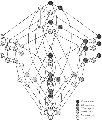
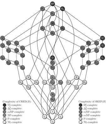
In the past, various semantic and syntactic restrictions have been proposed in order to identify computationally easier or even tractable fragments (see,e.g., [Sti90,KS91,BEZ02]). This is the starting point of the present paper. We propose a systematic study of fragments of default logic defined by restricting the set of allowed propositional connectives. For instance, if we look at the fragment where we forbid negation and the constant 0 and allow only conjunction and disjunction, we show that while the first problem is trivial (there always is an extension, in fact a unique one), the second and third problem become coNP-complete. In this paper we look at all possible sets B of propositional connectives and study the three decision problems investigated by Gottlob when all involved formulae contain only connectives from B. The computational complexity of the problems then, of course, becomes a function of B. We will see that Post’s lattice of all closed classes of Boolean functions is the right way to study all such sets B. Depending on the location of B in this lattice, we completely classify the complexity of all three reasoning tasks, see Figs. 1 and 2. We will show that, depending on the set B of occurring connectives, the problem of determining the existence of an extension is either Σp₂-complete, ∆p₂-complete, NP-complete, P-complete, NL-complete, or trivial, while for the reasoning problems the trivial cases split up into coNP-complete, P-complete, and NL-complete ones (under constant-depth reductions).

The motivation behind our approach lies in the hope that identifying frag-ments of default logic with simpler reasoning procedures may help us to under-stand the sources of hardness for the full problem and to locate the boundary between hard and easy fragments. In particular, these procedures may lead to algorithms for solving the studied problems more efficiently.

BF

R₁ R₀

R₂

M

M₁ M₀

M₂ S2

0 S2

02 S201 S3

0

S2 00 S3

02 S301 S3

00 S₀

S₀₂ S₀₁ S₀₀

D

D₁ D₂

V

V₁ V₀

V₂

L

L₁ L₃ L₀ L₂

N

N₂

I

I₁ I₀

I₂

S2 1

S2 12 S2

11

S3 1

S2 10

S3 12 S3

11 S3

10

S₁

S₁₂ S₁₁ S₁₀

E

E₀ E₁

E₂

trivial NL-complete P-complete NP-complete ∆p

2-complete

Σp2-complete

Complexity of SKEP(B):

Fig. 1.Post’s lattice. Colours indicate the complexity of EXT(B), the Extension Existence Problem forB-formulae.

2 Preliminaries

In this paper we make use of standard notions of complexity theory. The arising complexity degrees encompass the classes NL, P, NP, coNP, Σp₂ and Πp₂. For a thorough introduction into the field, the reader is referred to [Pap94]. For the hardness results, we useconstant-depth reductions, defined as follows: A language A is constant-depth reducible to a language B (A ≤cd B) if there

exists a logtime-uniform AC0-circuit family {Cn}n≥0 with unbounded fan-in {∧,∨,¬}-gates and oracle gates forB such that for allx, C_|x|(x) = 1 if and only ifx∈A (cf. [Vol99]).

BF

R₁ R₀

R₂

M

M₁ M₀

M₂ S2

0 S2

02 S201 S3

0

S2 00 S3

02 S301 S3

00 S₀

S₀₂ S₀₁ S₀₀

D

D₁ D₂

V

V₁ V₀

V₂

L

L₁ L₃ L₀ L₂

N

N₂

I

I₁ I₀

I₂ S2 1 S2 12 S2 11 S3 1 S2 10 S3 12 S3 11 S3 10 S₁ S₁₂ S₁₁ S₁₀ E E₀ E₁ E₂

Complexity of SKEP(B):

NL-complete P-complete coNP-complete coNP-complete ∆p 2-complete

Πp2-complete

Complexity of CRED(B):

NL-complete P-complete NP-complete coNP-complete ∆p 2-complete

Σp2-complete

Fig. 2.Post’s lattice. Colours indicate the complexity of CRED(B) and SKEP(B), the Credu-lous and Skeptical Reasoning Problems forB-formulae.

a variablex, we defineℓ as the literal of opposite polarity,i.e., ℓ:=x if ℓ=¬x

andℓ:=¬x ifℓ=x. For a formula ϕ, let ϕ[α/β] denoteϕwith all occurrences

of the formula α replaced by the formulaβ, and letA_[α/β]:={ϕ[α/β]|ϕ∈A}

forA⊆ L.

3 Boolean Clones and the Complexity of the Implication Problem

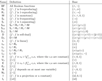
Name Definition Base

BF All Boolean functions {∧,¬}

R_{0 {}f:f is 0-reproducing} {∧,6→}

R₁ {f:f is 1-reproducing} {∨,→}

M _{f:f is monotone} {∨,∧,0,1}

S₀ {f:f is 0-separating} {→}

S_{1 {}f:f is 1-separating} {6→}

S00 S0∩R0∩R1∩M {x∨(y∧z)} S₁₀ S₁∩R₀∩R₁∩M {x∧(y∨z)}

S₁₁ S_1∩M _{{x∧(y∨z),0}}

D {f:f is self-dual} {(x∧y)∨(x∧z)∨(y∧z)}

D₂ D_∩M _{(x∧y)∨(y∧z)∨(x∧z)}

L {f:f is linear} {⊕,1}

L₀ L_∩R_{0 {⊕}}

L1 L∩R1 {≡}

L₂ L_∩R_0∩R_{1 {}x⊕y⊕z}

L₃ L_∩D _{{x⊕y⊕z,¬}}

V {f:f≡c0∨Wni=1cixiwhere thecis are constant} {∨,0,1}

V_{2 [{∨}] {∨}}

E {f:f≡c0∧Vni=1cixiwhere thecis are constant} {∧,0,1}

E_{2 [{∧}] {∧}}

N {f:f depends on at most one variable} {¬,0,1}

N_{2 [{¬}] {¬}}

I {f:f is a projection or a constant} {id,0,1}

I_{2 [{}id}] {id}

Table 1.A list of Boolean clones with definitions and bases.

arbitrary composition [Pip97, Chapter 1]. For an arbitrary set B of Boolean functions, we denote by [B] the smallest clone containingB and callB a base

for [B]. In [Pos41] Post classified the lattice of all clones and found a finite base for each clone, see Fig. 1. In order to introduce the clones relevant to this paper, we define the following notions forn-ary Boolean functions f:

– f is c-reproducing iff(c, . . . , c) =c,c∈ {0,1}.

– f is monotone if a1 ≤ b1, a2 ≤ b2, . . . , an ≤ bn implies f(a1, . . . , an) ≤

f(b1, . . . , bn).

– f isc-separating if there exists an i∈ {1, . . . , n}such thatf(a1, . . . , an) =c

implies ai =c,c∈ {0,1}.

– f isself-dual iff ≡dual(f), where dual(f)(x1, . . . , xn) =¬f(¬x1, . . . ,¬xn).

– f is linear if f ≡x1⊕ · · · ⊕xn⊕c for a constantc ∈ {0,1} and variables

x1, . . . , xn.

The clones relevant to this paper are listed in Table 1. The definition of all Boolean clones can be found, e.g., in [BCRV03].

For a finite set B of Boolean functions, we define the Implication Problem

forB-formulae IMP(B) as the following computational task: Given a set A of

B-formulae and aB-formulaϕ, decide whetherA|=ϕholds. The complexity of the implication problem is classified in [BMTV09a]. The results relevant to this paper are summarized in the following theorem.

1. coNP-complete if S_00⊆[B], S_{10⊆[B] or} D_{2⊆[B], and}

2. in P for all other cases.

4 Default Logic

Fix some finite set B of Boolean functions and let α, β, γ be propositional

B-formulae. A B-default (rule) is an expression d= α_γ:β; α is called prerequisite,

β is calledjustification and γ is called consequent ofd. A B-default theory is a pair hW, Di, where W is a set of propositionalB-formulae andD is a finite set of B-default rules. Henceforth we will omit the prefix “B-” if B = BF _{or the}

meaning is clear from the context.

For a given default theory hW, Di and a set of formulae E, let Γ(E) be the smallest set of formulae such that

1. W ⊆Γ(E),

2. Γ(E) is closed under deduction, i.e., Γ(E) = Th(Γ(E)), and

3. for all defaults α_γ:β ∈D withα∈Γ(E) and¬β /∈E, it holds thatγ ∈Γ(E).

A(stable) extensionofhW, Diis a fix-point of Γ,i.e., a setEsuch thatE = Γ(E). The following theorem by Reiter provides an alternative characterization of extensions:

Theorem 4.1 ([Rei80]). Let hW, Di be a default theory and E be a set of formulae.

1. Let E0=W and Ei+1 = Th(Ei)∪γ



α_γ:β ∈D, α∈E_i and¬β /∈E .Then E is a stable extension of hW, Di if and only if E =S

i∈NEi.

2. Let G = _α:β

γ ∈ D



α ∈ E and ¬β /∈ E . If E is a stable extension of hW, Di, then

E= Th(W ∪ {γ | α_γ:β ∈G}).

In this case, G is also called the set of generating defaults for E.

Observe that, as an immediate consequence of Theorem 4.1, stable exten-sions possess polynomial-sized witnesses, namely the set of their generating defaults. Moreover, note that stable extensions need not be consistent. However, the following proposition shows that this only occurs if the set W is already inconsistent.

Proposition 4.2 ([MT93, Corollary 3.60]). Let hW, Di be a default theory. Then L is a stable extension of hW, Di if and only if W is inconsistent.

As a consequence we obtain:

Corollary 4.3. Let hW, Di be a default theory.

– If W is consistent, then every stable extension of hW, Di is consistent.

– If W is inconsistent, then hW, Di has a stable extension.

1. theExtension Existence Problem EXT(B)

Instance: aB-default theory hW, Di

Question:DoeshW, Di have a stable extension? 2. theCredulous Reasoning Problem CRED(B)

Instance: aB-formulaϕand a B-default theory hW, Di

Question:Is there a stable extension ofhW, Di that includesϕ? 3. theSkeptical Reasoning Problem SKEP(B)

Instance: aB-formulaϕand a B-default theory hW, Di Question:Does every stable extension of hW, Di include ϕ?

The next theorem follows from [Got92] and states the complexity of the above decision problems for the general case [B] =BF_.

Theorem 4.4. Let B be a finite set of Boolean functions such that [B] =

BF_{. ThenEXT(B) and CRED(B) are Σ}p

2-complete, whereas SKEP(B) is Πp2

-complete.

Proof. The upper bounds given in [Got92] do not depend on the Boolean connectives allowed and thus hold for any finite set B of Boolean functions. For Σp₂- and Πp₂-hardness, it suffices to note that if [B] =BF_{, then there exist} B-formulaef(x, y),g(x, y) andh(x) such that f(x, y)≡x∧y,g(x, y)≡x∨y,

h(x)≡ ¬xand both x andy occur at most once inf, g, and h [Lew79]. Hence, the hardness results generalize to arbitrary basesB with [B] =BF_.

5 The Complexity of Default Reasoning

In this section we will classify the complexity of the three problems EXT(B), CRED(B), and SKEP(B) for all choices of Boolean connectives B. We start with some preparations which will substantially reduce the number of cases we have to consider.

Lemma 5.1. LetP be any of the problems EXT, CRED, or SKEP. Then for each finite setB of Boolean functions, P(B)≡cdP(B∪ {1}).

Proof. The reductions P(B) ≤cd P(B ∪ {1}) are obvious. For the converse

reductions, we will essentially substitute the constant 1 by a new variable t

that is forced to be true (this trick goes back to Lewis [Lew79]). For EXT, the reduction is given byhW, Di 7→ hW′_{, D}′_{i, where W}′ _=W

[1/t]∪ {t},D′ =D[1/t],

andtis a new variable not occurring inhW, Di. If hW′_{, D}′_{i possesses a stable}

extensionE′, thent∈E′. Hence, E_[′_t/1] is a stable extension ofhW, Di. On the other hand, ifEis a stable extension ofhW, Di, then Th(E_[1/t]∪{t}) =E_[1/t]is a stable extension ofhW′_{, D}′_{i. Therefore, each extensionE ofhW, Di corresponds}

to the extensionE_[1/t] ofhW′, D′i, and vice versa.

For the problems CRED and SKEP, it suffices to note that the above reductionhW, Di 7→ hW′_{, D}′_{i has the additional property that for each formula} ϕand each extensionE of hW, Di,ϕ∈E if and only if ϕ_[1/t]∈E_[1/t].

Lemma 5.2. Let B be a finite set of Boolean functions. Let hW, Di be a B -default theory. If[B]⊆R_{1 thenhW, Dihas a unique stable extension. If [B]⊆}M

then hW, Di has at most one stable extension.

Proof. For [B]⊆R_{1, every premise, justification and consequent is 1-reproducing.}

As all consequences of 1-reproducing functions are again 1-reproducing and the negation of a 1-reproducing function is not 1-reproducing, the justifications inD

become irrelevant. Hence the characterization of stable extensions from the first item in Theorem 4.1 simplifies to the following iterative construction: E0 =W

and Ei+1 = Th(Ei)∪γ

 α:β

γ ∈D, α∈Ei .As D is finite, this construction

terminates after finitely many steps, i.e., Ek = Ek+1 for some k ≥ 0. Then E =S

i≤kEi is the unique stable extension ofhW, Di. For a similar result confer

[BO02, Theorem 4.6].

For [B]⊆M_{, every formula is either 1-reproducing or equivalent to 0. As}

rules with justification equivalent to 0 are never applicable, eachB-default theory

hW, Di with finiteDhas at most one stable extension by the same argument as

above.

As an immediate corollary, the credulous and the skeptical reasoning problem are equivalent for the above choices of the underlying connectives.

Corollary 5.3. Let B be a finite set of Boolean functions such that [B]⊆R₁

or [B]⊆M_{. ThenCRED(B)≡cdSKEP(B).}

Proof. For [B] ⊆ R_{1, CRED(B) ≡cd SKEP(B) trivially holds. For [B] ⊆} M_,

observe that a givenB-default theoryhW, Dipossesses a stable extension if and only if (hW, Di,1)∈CRED(B), possesses a consistent stable extension if and only if (hW, Di,0)∈/SKEP(B), and possesses the inconsistent stable extension if and only if (hW,∅i,0)∈SKEP(B).

Hence, we obtain (hW, Di, ϕ) ∈ SKEP(B) if and only if (hW, Di, ϕ) ∈

CRED(B) or (hW, Di,1)∈/ CRED(B); and, similarly, (hW, Di, ϕ)∈CRED(B) if and only if (hW, Di, ϕ)∈SKEP(B) and (hW, Di, p)∈/ SKEP(B)

or (hW,∅i, p)∈SKEP(B), where p is a fresh proposition.

5.1 The Extension Existence Problem

Now we are ready to classify the complexity of EXT. The next theorem shows that this is a hexachotomy: the Σp₂-completeness of the general case [Got92] is inherited by all clones above S_{1 and} D_{; for monotone sets of connectives}

the complexity drops to ∆p₂-completeness if ∧, ∨ and 0 are available, and membership in P otherwise (with this case splitting up into P-completeness, NL-completeness and triviality); lastly, for affine sets of connectives containing

¬ or 0 the complexity of EXT reduces to NP-completeness.

Theorem 5.4. Let B be a finite set of Boolean functions. Then EXT(B) is

1. Σp₂-complete if S_{1 ⊆[B]⊆}BF _or D_⊆[B]⊆BF_,

2. ∆p₂-complete if S_11⊆[B]⊆M_,

Algorithm 1 Determining the existence of a stable extension Require: hW, Di

1: Gnew←W 2: repeat

3: Gold←Gnew 4: for all α_γ:β ∈Ddo

5: if Gold|=αandβ6≡0then 6: if γ≡0then

7: return false

8: end if

9: Gnew←Gnew∪ {γ} 10: end if

11: end for

12: untilGnew=Gold 13: return true

4. P-complete if [B]∈ {E_,E_0,V_,V_0},

5. NL-complete if [B]∈ {I_,I_{0}, and}

6. trivial in all other cases (i.e., if [B]⊆R_1).

The proof of Theorem 5.4 will be established from the lemmas in this subsection.

Lemma 5.5. LetB be a finite set of Boolean functions such thatS_11⊆[B]⊆M_.

Then EXT(B) is ∆p₂-complete.

Proof. We start by showing EXT(B) ∈ ∆p₂. Let B be a finite set of Boolean functions such that [B]⊆M _{and hW, Di be a B-default theory. As the negated}

justification¬β of every default rule α_γ:β ∈Dis either equivalent to the constant 1 or not 1-reproducing, it holds that in the former case¬β is contained in any stable extension, whereas in the latter¬β cannot be contained in a consistent stable extension of hW, Di. We can distinguish between those two cases in polynomial time. Therefore, using the characterization of Theorem 4.1 (1), we can iteratively compute the applicable defaults and test whether the premise of any default with unsatisfiable conclusion can be derived. Algorithm 1 implements these steps on a deterministic Turing machine using a coNP-oracle to test for implication ofB-formulae. Clearly, Algorithm 1 terminates after a polynomial number of steps. Hence, EXT(B) is contained in ∆p₂.

To show the ∆p₂-hardness of EXT(B), we reduce from the ∆p₂-complete problem SNSAT [Got95a, Theorem 3.4] defined as follows:

Problem: SNSAT

Input: A sequence (ϕi₎

1≤i≤n of formulae such thatϕi contains the

propositions x1, . . . , xi−1 and zi1, . . . , zimi

Output: Is cn = 1, where ci is recursively defined via ci := 1 if

and only if ϕi is satisfiable by an assignment σ such that

σ(xj) =cj for all 1≤j < i?

predecessors. We will encode such an instance into a sequence of default rules such that the resulting default theory has a stable extension if and only if the last formula in the given instance of SNSAT is satisfiable, that is,cn= 1.

Let (ϕi)1≤i≤n be the given sequence of propositional formulae and assume

without loss of generality thatϕi _{is in conjunctive normal form for all 1≤i≤n.}

For every propositionxj or zij occurring in (ϕi)1≤i≤n, letx′_j respectively z_ij′ be

a fresh proposition, and define

ψi :=ϕi_[¬x

1/x′1,...,¬xi−1/x′i−1,¬zi1/zi′1,...,¬zimi/z′imi]∧

i−1 ^

j=1

(xj ∨x′j)∧ mi ^

j=1

(zij∨zij′ ).

The key observation in the relationship ofϕi andψiis that, for allc1, . . . , ci−1 ∈ {0,1}, ϕi

[x1/c1,...,xi−1/ci−1] is unsatisfiable if and only if for each model σ of

ψi

[x1/c1,...,xi−1/ci−1,x′1/¬c1,...,x′i−1/¬ci−1] there exists an index 1≤j≤mi such that

σ sets to 1 both zij and zij′ . We will use this observation to show that the

B-default theory hW, Di defined below has a stable extension if and only if (ϕi)1≤i≤n is an instance of SNSAT, that is, ϕn_{[x1/c1,...,xi−1/ci−1]} is satisfiable for

c1, . . . , ci−1 recursively defined via

ci := 1 ⇐⇒ ϕi[x1/c1,...,xi−1/ci−1] is satisfiable. (1)

Define W :={ψ1, . . . , ψn}and

D:=

( Wmi

j=1(zij∧zij′ )∨

Wi−1

j=1(xj∧x′j) : 1

x′

i

1≤i < n )

∪

( Wmn

j=1(znj∧z′nj)∨

Wn−1

j=1(xj ∧x′j) : 1

0

)

.

We will prove the claim appealing to the characterization of stable extensions from Theorem 4.1 (1). LetE0 :=W. If ϕ1 is unsatisfiable then

Wm₁

j=1(z1j∧z′1j):1

x′

1 is applicable and thus x′

1 is added to E1. On the other hand, if ϕ1 is satisfiable

then there exists a model σ of ϕ1. Define ˆσ as the extension of σ defined as ˆ

σ(z₁′_j) =¬σ(z1j) for all 1≤j≤m1. By virtue ofσ |=ϕ1 and the construction

of ˆσ, we obtain that ˆσ |= ψ1 while ˆσ 6|= Wm1

j=1(z1j ∧z1′j). Summarizing, ϕ1 is

unsatisfiable if and only if Wm1

j=1(z1j∧z1′j):1

x′

1 is applicable.

Now suppose thatEi is such that for allj < ithe propositionx′j is contained

in Ei if and only if ϕj_{[x1/c1,...,xj−1/cj−1]} with c1, . . . , cj−1 defined as in (1) is

unsatisfiable. Ifϕi

[x1/c1,...,xi−1/ci−1] is unsatisfiable then any model of the formula

ψi∧ ^ 1≤j<i,

cj=1 xj∧

^

1≤j<i, cj=0

x′_j (2)

sets to 1 bothzij andzij′ for some 1≤j≤mi. From (2) and the monotonicity of

ψi, we obtain that for each modelσ′ofψi∧V

an index 1≤ j < i such thatσ′ sets xj and x′j to 1, or an index 1≤j ≤mi

such that σ′ sets zij and zij′ to 1. Consequently,

Wmi

j=1(zij∧zij′ )∨

Wi−1

j=1(xj∧x′j):1

x′

i is

applicable andx′_i ∈Ei+1. On the other hand, if ϕi_{[x1/c1,...,xi−1/ci−1]} is satisfiable

then there exists a modelσ that can be extended to ˆσ by ˆσ(z′_ij) =¬σ(zij) for

all 1 ≤ j ≤ mi and ˆσ(x′j) = ¬σ(xj) for all 1 ≤ j < i such that ˆσ |= ψi and

ˆ

σ6|=Wmi

j=1(zij∧zij′ )∨

Wi−1

j=1(xj∧x′j). Summarizing,ϕi is unsatisfiable if and only

if Wmi

j=1(zij∧z′ij)∨

Wi−1

j=1(xj∧x′j):1

x′

i is applicable.

The direction from right to left now follows from the fact thatϕnis satisfiable

if and only if Wmn

j=1(zij∧zij′ )∨

Wn−1

j=1(xi∧x′i):1

0 is not applicable, which in turn implies

thathW, Dihas a stable extension. Conversely, ifϕn_[x

1/c1,...,xn−1/cn−1] is unsatisfi-able withc1, . . . , cn−1 defined as in (1), then any model ofψi∧V1≤j<i,σ(cj)=0x′j

sets to true eitherxj andx′j for some 1≤j < iorzij andzij′ for some 1≤j≤mi.

As a result, the default Wmn

j=1(zij∧z′ij)∨

Wn−1

j=1(xj∧x′j):1

0 is applicable and hW, Di does

not possess a stable extension.

Finally, observe that all formulae contained inhW, Di are monotone. Hence,

hW, Di is a{∧,∨,0,1}-default theory. LetB be a finite set of Boolean functions such thatS_{11⊆[B]. Replacing all occurrences ofx∧y andx∨yin hW, Di with}

their respective (B∪ {1})-representations f∧(x, y) andf∨(x, y), and eliminating

the constant 1 as in the proof of Lemma 5.1 yields aB-default theoryhWB_{, D}B_i

that is equivalent tohW, Di. The variables x or y may occur several times in the body off∧ or f∨, hence hWB, DBi might be exponential in the length of

the original input. To avoid this blowup, we exploit the associativity of∧ and

∨: we insert parentheses such that the conjunctions and disjunctions in each of the above formulae are transformed into trees of logarithmic depth.

Thus we have established a reduction from SNSAT to EXT(B) for all B

such thatS_{11⊆[B]. This concludes the proof.}

Lemma 5.6. Let B be a finite set of Boolean functions such that[B]∈ {N_,N_2, L_,L_0,L_{3}. Then EXT(B) isNP-complete.}

Proof. We start by showing EXT(B)∈NP for [B]⊆L_{. Given a default theory} hW, Di, we first guess a set G ⊆ D which will serve as the set of generating defaults for a stable extension. LetG′=W∪ {γ | α_γ:β ∈G}. We use Theorem 4.1 to verify whether Th(G′) is indeed a stable extension of hW, Di. For this we inductively compute generators Gi for the sets Ei from Theorem 4.1, until

eventuallyEi =Ei+1 (note, that becauseD is finite, this always occurs). We

start by settingG0 =W. Given Gi, we check for each rule α_γ:β ∈D, whether

Gi |= α and G′ 6|= ¬β (as all formulae belong to L(B), this is possible by

Theorem 3.1). If so, then γ is put intoGi+1. If this process terminates, i.e., if Gi =Gi+1, then we check whetherG′ =Gi. By Theorem 4.1, this test is positive

if and only ifG generates a stable extension of hW, Di.

To show NP-hardness of EXT(B) for N _{⊆ [B], we will ≤cd-reduce 3SAT}

to EXT(B). Let ϕ=Vn

hW, Dϕi, whereW :=∅ and

Dϕ :=

1 :xi

xi

   

1≤i≤m

∪

1 :¬xi

¬xi

 

1≤i≤m

∪

_ℓ

iπ(1):ℓiπ(2) ℓiπ(3)

   

1≤i≤n, π is a permutation of {1,2,3}

.

To prove the correctness of the reduction, first assumeϕto be satisfiable. For each satisfying assignmentσ :{x1, . . . , xm} → {0,1}forϕ, we claim that

E := Th({xi|σ(xi) = 1} ∪ {¬xi |σ(xi) = 0})

is a stable extension of hW, Dϕi. We will verify this claim with the help of the

first part of Theorem 4.1. Starting with E0 =∅, we already getE1 =E by the

default rules 1:xi

xi and 1:¬xi

¬xi in Dϕ. As σ is a satisfying assignment for ϕ, each

consequent of a default rule inDϕ is already inE. HenceE2 =E1 and therefore E =S

i∈NEi is a stable extension of hW, Dϕi.

Conversely, assume that E is a stable extension ofhW, Dϕi. Because of the

default rules 1:xi

xi and 1:¬xi

¬xi , we either getxi∈E or ¬xi∈E for all i= 1, . . . , m.

The rules of the type ℓi1:ℓi2

ℓi3 ensure that E contains at least one literal from each clause ℓi1 ∨ℓi2∨ℓi3 in ϕ. As E is deductively closed, E contains ϕ. By

Corollary 4.3, the extension E is consistent, and therefore ϕis satisfiable. Hence, EXT(B) is NP-complete for every finite setB such that N_⊆[B]⊆ L_{. The remaining cases [B] ∈ {}N_2,L_0,L_{3} follow from Lemma 5.1, because}

[N_{2∪ {1}] =}N_{, [}L_{0∪ {1}] =}L_{, and [}L_{3∪ {1}] =}L_.

Lemma 5.7. Let B be a finite set of Boolean functions such that [B]∈ {E_,E_0, V_,V_{0}. Then EXT(B) isP-complete.}

Proof. Let B be a finite set of Boolean functions such that [B]∈ {E_,E_0,V_,V_0}.

Then, [B]⊆M_{. Consequently, membership in P is obtained from Algorithm 1,}

as for these types of B-formulae, we have an efficient test for implication. To prove P-hardness forE_{0⊆[B], we provide a reduction from the}

comple-ment of the accessibility problem for directed hypergraphs, HGAP. In directed hypergraphs H = (V, F), hyperedges e ∈ F consist of a set of source nodes src(e) ⊆ V and a destination dest(e) ∈ V. Instances of HGAP contain a di-rected hypergraph H= (V, F), a setS ⊆V of source nodes, and a target node

t∈V. HGAP is P-complete under ≤cd-reductions [SI90], even if restricted to

hypergraphs whose edges contain at most two source nodes.

We transform a given instance (H, S, t) to the EXT({∧,0,1})-instancehW, Di

with

W :={ps |s∈S}, D:=

V

v∈src(e)pv : 1

p_dest(e)

e∈F

∪

pt: 1

0

with pairwise distinct propositions pv for v ∈ V. It is easy to verify that

setsB such thatE_{0 ⊆[B]. As P is closed under complementation, EXT(B) is}

P-complete.

ForV_{0 ⊆[B], set}

W :=n _

s /∈S

ps

o , D:=

W

v∈V\src(e)pv : 1 W

v∈V\(src(e)∪{dest(e)})pv

e∈F

∪ W

v∈V\{t}pv : 1

0

.

We claim that this mapping realizes the reduction HGAP≤cdEXT({∨,0,1}).

First suppose that tcan be reached from S inH. Then there exists a sequence (Si)0≤i≤n of sets of nodes such thatS0 =S,t∈Sn, and for all 0≤i < n,Si+1

is obtained fromSi by adding the destination dest(e) of a hyperedge e∈F with

src(e)⊆Si. Let (ei)0≤i<ndenote the corresponding sequence of hyperedges used

to obtain Si+1 from Si. Then, for all 0≤i < n, the following holds:

src(ei)⊆Si ⇐⇒

W

v∈V\src(e)pv : 1 W

v∈V\(src(e)∪{dest(e)})pv

is applicable inEi,

where (Ei)i∈N is the sequence from Theorem 4.1 (1). AsS_i∈NE_i is guaranteed

to be unique by Lemma 5.2 andt∈Sn, we obtain that 0∈En+1. Consequently, hW, Di does not possess a stable extension.

Conversely, if hW, Di does not admit a stable extension, then 0 has to be derivable. Accordingly, there exists a sequence of defaults (di)0≤i≤n such that

the premise of di can be derived from W ∪γ

d_j = α_γ:β,0 ≤ j < i and

dn=

W

v∈V\{t}pv:1

0 . By construction of hW, Di, this sequence can be translated

into a sequence (Si)0≤i≤n of node sets in the hypergraph such that S0 = S, t∈Sn, and for all 0≤i < n, Si+1 is obtained fromSi by adding the destination

dest(e) of a hyperedgee∈F with src(e)⊆Si. Consequently,tis reachable from

S in H and we conclude that HGAP≤cdEXT({∨,0,1}). Using Lemma 5.1, we

get HGAP≤cdEXT({∨,0}).

To see that EXT({∨,0})≤cdEXT(B) for all finite setsB such thatV0 ⊆[B],

we proceed as in the proof of Lemma 5.5 and insert parentheses such that the disjunctions in each of the above formulae are transformed into tree of logarithmic depth. Hence, replacing all occurrences of∨in W, Dandϕwith its

B-representation yields an EXT(B)-instance of size polynomial in the original input. Concluding, EXT(B) is P-complete.

Lemma 5.8. Let B be a finite set of Boolean functions such that [B]∈ {I_,I_0}.

Then EXT(B) is NL-complete with respect to constant-depth reductions.

Proof. LetB be a finite set of Boolean functions such that [B]∈ {I_,I_{0}. We will}

first show membership in NL by giving a reduction to the complement of the graph accessibility problem, GAP.

LethW, Dibe aB-default theory. Analogously to the proof of Lemma 5.5, it holds thathW, Di has a stable extension if and only if either W is inconsistent or the conclusions of all applicable defaults are consistent. Assume thatW is consistent and denote by D′ ⊆Dthose defaults α_γ:β ∈D with β 6≡0. Then a

in W or itself the conclusion of an applicable default. Therefore, testing whether the conclusions of all applicable defaults are consistent is essentially equivalent to solving a reachability problem in a directed graph. Define GhW,Di as the

directed graph (V, F) with

V :={0,1} ∪W ∪nα, γ

α:β

γ ∈D

o ,

F :={(1, x)|x∈W} ∪n(α, γ)

α:β

γ ∈D, β6≡0

o

ifW is consistent, and

V :={0,1}, F :=∅

otherwise. It is easy to see thathW, Dihas a stable extension if and only if there is no path from 1 to 0 inG_hW,Di. Thus the function mapping the givenB-default theory hW, Di to the GAP-instance (G_hW,Di,1,0) constitutes a reduction from EXT(B) to GAP. As the consistency of W can be determined in AC0, the reduction can be computed using constant-depth circuits. Membership in NL follows from the closure of NL under complementation.

To show NL-hardness, we establish a constant-depth reduction in the converse direction. For a directed graphG= (V, F) and two nodess, t∈V, we transform the given GAP-instance (G, s, t) to hW, Di with

W :={ps}, D:=

n

pu:pu

pv

(u, v)∈F o

∪npt:pt 0

o

Clearly, (G, s, t)∈GAP if and only if hW, Di does not have a stable extension. As NL is closed under complementation, the lemma is established.

Proof (Theorem 5.4). For S_1⊆[B]⊆BF_{or [B] =}D_{, observe that in both cases} BF_{= [B∪ {1}]. Claim 1 then follows from Theorem 4.4 and Lemma 5.1. Claims}

two to five are established in Lemmas 5.5–5.8. For all sets B not captured by the above, it now holds that [B]⊆R_{1. Thus, the sixth claim follow directly from}

Lemmas 5.2,

5.2 The Credulous and the Skeptical Reasoning Problem

otherwise. Conversely, if the implication problem becomes easy but determining an extension candidate is hard, then CRED(B) is NP-complete, while SKEP(B) is coNP-complete. This is the case for [B]∈ {N_,N_2,L_,L_0,L_{3}. Finally, for clones} B that allow for solving both tasks in polynomial time, both CRED(B) and SKEP(B) are in P.

The complete classification of CRED(B) is given in the following theorem.

Theorem 5.9. Let B be a finite set of Boolean functions. Then CRED(B) is

1. Σp₂-complete if S_1⊆[B]⊆BF _or D_⊆[B]⊆BF_,

2. ∆p₂-complete if S_11⊆[B]⊆M_,

3. coNP-complete if X⊆[B]⊆R_{1 for X ∈ {}S_00,S_10,D_2},

4. NP-complete if [B]∈ {N_,N_2,L_,L_0,L_3},

5. P-complete if V_{2 ⊆[B]⊆}V_, E_{2 ⊆[B]⊆}E _{or [B]∈ {}L_1,L_{2}, and}

6. NL-complete if I_{2 ⊆[B]⊆}I_.

The proof of Theorem 5.9 follows from the upper and lower bounds given in Propositions 5.10 and 5.11 below.

Proposition 5.10. Let B be a finite set of Boolean functions. ThenCRED(B)

is contained

1. in ∆p₂ if [B]⊆M_,

2. in coNP if [B]⊆R_1,

3. in NP if [B]⊆L_,

4. in P if [B]⊆V_{, [B]⊆}E _{or [B]⊆}L_{1, and}

5. in NLif [B]⊆I_.

Proof. For [B] ⊆ M_{, membership in ∆}p

2 is obtained from a straightforward

extension of Algorithm 1: first iteratively compute the applicable defaultsG

while asserting that hW, Di has a stable extension using Algorithm 1, and eventually verify thatϕis implied byW and the conclusions in G.

For [B] ⊆ R_{1, the justifications β are irrelevant for computing a stable}

extension, as for every default rule α_γ:β ∈ D we cannot derive ¬β (¬β is not 1-reproducing). Hence, for any default theory hW, Di a unique consistent stable extensionE is guaranteed to exist. Using Algorithm 1 we can iteratively compute the generating defaults of this stable extension and eventually check whetherϕ

is implied byW and the conclusions of the generating defaults of E.

For [B] ⊆ L_{, we proceed similarly as in the proof of Lemma 5.6. First,}

we guess a set G of generating defaults and subsequently verify that both Th(W ∪ {γ | α_γ:β ∈G}) is a stable extension and thatW ∪ {γ | α_γ:β ∈G} |=ϕ. Using Theorem 3.1, both conditions may be verified in polynomial time.

For [B]⊆V_{, [B]⊆}E_{, and [B]⊆}L_{1, we again use Algorithm 1. As for these}

types ofB-formulae we have an efficient test for implication (Theorem 3.1), we get CRED(B)∈P.

For [B] ⊆I_{, observe that NL is closed under intersection. Hence, given a} B-default theoryhW, Di and a B-formula ϕwe can first test whether hW, Di

has a stable extensionE using Lemma 5.8 and subsequently assert thatϕ∈E

by reusing the graph G_hW,Di constructed from hW, Di: it holds that ϕ∈ E if and only if the node corresponding toϕis contained inGhW,Di and reachable

We will now establish the lower bounds required to complete the proof of Theorem 5.9.

Proposition 5.11. LetB be a finite set of Boolean functions. Then CRED(B)

is

1. Σp₂-hard if S_{1 ⊆[B]or} D_⊆[B],

2. ∆p₂-hard if S_11⊆[B],

3. coNP-hard if S_00⊆[B], S_10⊆[B]or D_{2 ⊆[B],}

4. NP-hard if N_{2 ⊆[B]or} L_{0 ⊆[B],}

5. P-hard ifV_{2 ⊆[B],} E_{2 ⊆[B]or} L_{2 ⊆[B], and}

6. NL-hard for all other clones.

Proof. Part one follows from Theorem 4.4 and Lemma 5.1.

For the second part, observe that the constant 1 is contained in any stable extension. The second part thus follows from Lemmas 5.1 and 5.5.

ForS_00⊆[B], S_{10⊆[B], and}D_{2 ⊆[B], coNP-hardness is established by a} ≤cd-reduction from IMP(B). Let A⊆ L(B) and ϕ∈ L(B). Then the default

theoryhA,∅ihas the unique stable extension Th(A), and henceA|=ϕif and only if (hA,∅i, ϕ) ∈ CRED(B). Therefore, IMP(B) ≤cd CRED(B), and the

claim follows with Theorem 3.1.

For the fourth part, it suffices to prove NP-hardness for N_{2 ⊆ [B]. For} L_{0 ⊆ [B], the claim then follows by Lemma 5.1. For} N_{2 ⊆ [B], we obtain}

NP-hardness of CRED(B) by adjusting the reduction given in the proof of Lemma 5.6. Consider the mapping ϕ7→(h{ψ}, Dϕi, ψ), whereDϕ is the set of

default rules constructed fromϕin Theorem 5.4, andψis a satisfiableB-formula such that ϕ andψ do not use common variables. By Theorem 5.4,ϕ∈3SAT if and only if h{ψ}, Dϕi has a stable extension. As any extension ofh{ψ}, Dϕi

containsψ, we obtain 3SAT≤cdCRED(B) via the above reduction.

For the fifth part, the casesE_{2 ⊆ [B] and} V_{2 ⊆[B] follow similarly from}

Lemmas 5.1 and 5.7. It hence suffices to prove the P-hardness for L_{2 ⊆[B]. We}

again provide a reduction from HGAP restricted to hypergraphs whose edges contain at most two source nodes. To this end, we transform a given instance (H, S, t) with H = (V, F), to the CRED({x⊕y⊕z,1})-instance (hW, Di, ϕ),

where

W :={ps|s∈S},

D:=

_p

src(e) : 1 pdest(e)

   

e∈F,|src(e)|= 1

∪

_p

src1(e): 1

pe

,psrc2(e): 1

pe

,psrc1(e)⊕psrc2(e)⊕pe: 1

pdest(e)

   

e∈F,|src(e)|= 2

,

ϕ:=pt,

and{src1(e),src2(e)}denote the source nodes ofe. As for the correctness, observe

that if for somee∈F with |src(e)|= 2 both variablesp_src1(e) andp_src2(e)can be derived from the stable extension ofhW, Di, thenpe and consequentlypdest(e)

none or two of the propositions inp_src1(e)⊕psrc2(e)⊕peare satisfied. Thuspdest(e) cannot be derived from the defaults corresponding toe.

Finally, it remains to show NL-hardness forI_{2 ⊆[B]. We give a≤cd-reduction}

from GAP to CRED({id}). For a directed graph G = (V, F) and two nodes

s, t ∈ V, we transform the GAP-instance (G, s, t) with G = (V, F) to the CRED(I_2)-instance

W :={ps}, D:=

pu :pu

pv

   

(u, v)∈F

, ϕ:=pt.

Clearly, (G, s, t)∈GAP if and only if ϕis contained in all stable extensions of

hW, Di.

This completes the proof of Theorem 5.9.

We will next classify the complexity of the skeptical reasoning problem. The analysis as well as the result are similar to the classification of the credulous reasoning problem (cf. also Fig. 2).

Theorem 5.12. Let B be a finite set of Boolean functions. Then SKEP(B) is

1. Πp₂-complete if S_{1 ⊆[B]⊆}BF _or D_⊆[B]⊆BF_,

2. ∆p₂-complete if S_11⊆[B]⊆M_,

3. coNP-complete if X ⊆ [B] ⊆ Y, where X ∈ {S_00,S_10,N_2,L_{0} and Y ∈} {R_1,M_,L_},

4. P-complete if V_{2 ⊆[B]⊆}V_, E_{2 ⊆[B]⊆}E _{or [B]∈ {}L_1,L_{2}, and}

5. NL-complete if I_{2 ⊆[B]⊆}I_.

Proof. The first part again follows from Theorem 4.4 and Lemma 5.1.

For [B]∈ {N_,N_2,L_,L_0,L_{3}, we guess similarly as in Theorem 5.4 a set Gof}

defaults and then verify in the same way whetherW andGgenerate a stable extensionE. If not, then we accept. Otherwise, we check if E|=ϕand answer according to this test. This yields a coNP-algorithm for SKEP(B). Hardness for coNP is achieved by modifying the reduction from Theorem 5.4 (cf. also the proof of Proposition 5.11): mapϕto (h∅, Dϕi, ψ), where Dϕ is defined as in the

proof of Theorem 5.4, andψ is a non-tautologicalB-formula such that ϕandψ

do not share variables. Thenϕ /∈3SAT if and only if h∅, Dϕi does not have a

stable extension. The latter is true if and only ifψ is in all extensions ofh∅, Dϕi.

Hence 3SAT≤cdSKEP(B), establishing the claim.

For all remaining clones B, observe that [B] ⊆ R_{1 or [B] ⊆} M_{. Hence,}

Corollary 5.3 and Theorem 5.9 imply the claim.

6 Conclusion

but easy for SAT). The complexity of the membership problems, i.e., credu-lous and skeptical reasoning, rests on two sources: first, whether there exists a unique extension (cf. Lemma 5.2), and second, how hard it is to test for formula implication. For this reason, we also classified the complexity of the implication problem IMP(B).

A different complexity classification of reasoning for default logic has been undertaken in [CHS07]. In that paper, the language of existentially quantified propositional logic was restricted to so called conjunctive queries,i.e., existen-tially quantified formulae in conjunctive normal-form with generalized clauses. The complexity of the reasoning tasks was determined depending on the type of clauses that are allowed. We want to remark that though our approach at first sight seems to be more general (since we do not restrict our formulae to CNF), the results in [CHS07] do not follow from the results presented here (and vice versa, our results do not follow from theirs).

In the light of our present contribution, it is interesting to remark that by results of Konolige, Gottlob, and Janhunen [Kon88,Got95b,Jan99], proposi-tional default logic and Moore’s autoepistemic logic are essentially equivalent. Even more, the translations are efficiently computable. Unfortunately, all of them require a complete set of Boolean connectives, whence our results do not immediately transfer to autoepistemic logic. It is nevertheless interesting to ask whether the exchange of default rules with the introspective operatorL yields hitherto unclassified fragments of autoepistemic logic that allow for efficient stable expansion testing and reasoning.

Acknowledgements

We thank Ilka Schnoor for sending us a manuscript with the proof of the NP-hardness of EXT(B) for all B such that N_{2 ⊆[B]. We also acknowledge helpful}

discussions on various topics of this paper with Peter Lohmann.

References

[BCRV03] E. B¨ohler, N. Creignou, S. Reith, and H. Vollmer. Playing with Boolean blocks, part I: Post’s lattice with applications to complexity theory. SIGACT News, 34(4):38–52, 2003.

[BEZ02] R. Ben-Eliyahu-Zohary. Yet some more complexity results for default logic.

Artificial Intelligence, 139(1):1–20, 2002.

[BMTV09a] O. Beyersdorff, A. Meier, M. Thomas, and H. Vollmer. The complexity of propositional implication. Information Processing Letters, 109(18):1071–1077, 2009.

[BMTV09b] O. Beyersdorff, A. Meier, M. Thomas, and H. Vollmer. The complexity of reasoning for fragments of default logic. InProc. 12th International Conference on Theory and Applications of Satisfiability Testing, volume 5584 ofLecture Notes in Computer Science, pages 51 – 64. Springer Verlag, 2009.

[BO02] P. A. Bonatti and N. Olivetti. Sequent calculi for propositional nonmonotonic logics. ACM Transactions on Computational Logic, 3(2):226–278, 2002.

[CHS07] P. Chapdelaine, M. Hermann, and I. Schnoor. Complexity of default logic on generalized conjunctive queries. InProc. 9th International Conference on Logic

Programming and Nonmonotonic Reasoning, volume 4483 ofLecture Notes in

[GL91] M. Gelfond and V. Lifschitz. Classical negation in logic programs and disjunctive databases. New Generation Comput., 9(3/4):365–386, 1991.

[Got92] G. Gottlob. Complexity results for nonmonotonic logics. Journal of Logic Com-putation, 2(3):397–425, 1992.

[Got95a] G. Gottlob. NP trees and Carnap’s modal logic. Journal of the ACM, 42(2):421– 457, 1995.

[Got95b] G. Gottlob. Translating default logic into standard autoepistemic logic. Journal of the ACM, 42(4):711–740, 1995.

[Jan99] T. Janhunen. On the intertranslatability of non-monotonic logics. Annals of Mathematics and Artificial Intelligence, 27(1-4):79–128, 1999.

[Kon88] K. Konolige. On the relation between default and autoepistemic logic. Artificial Intelligence, 35(3):343–382, 1988. Erratum: Artificial Intelligence, 41(1):115. [KS91] H. A. Kautz and B. Selman. Hard problems for simple default logics. Artificial

Intelligence, 49:243–279, 1991.

[Lew79] H. Lewis. Satisfiability problems for propositional calculi. Mathematical Systems Theory, 13:45–53, 1979.

[McC80] J. McCarthy. Circumscription – a form of non-monotonic reasoning. Artificial Intelligence, 13:27–39, 1980.

[MT93] V. W. Marek and M. Truszczy´nski. Nonmonotonic Logic. Artificial Intelligence. Springer Verlag, Berlin Heidelberg, 1993.

[Pap94] C. H. Papadimitriou. Computational Complexity. Addison-Wesley, Reading, MA, 1994.

[Pip97] N. Pippenger.Theories of Computability. Cambridge University Press, Cambridge, 1997.

[Pos41] E. Post. The two-valued iterative systems of mathematical logic. Annals of Mathematical Studies, 5:1–122, 1941.

[Rei80] R. Reiter. A logic for default reasoning. Artificial Intelligence, 13:81–132, 1980. [SI90] R. Sridhar and S. Iyengar. Efficient parallel algorithms for functional dependency

manipulations. InProc. 2nd International Symposium on Databases in Parallel and Distributed Systems, pages 126–137. ACM, 1990.

[Sti90] J. Stillman. It’s not my default: The complexity of membership problems in restricted propositional default logics. In Proc. 8th Conference on Artificial Intelligence, pages 571–578. ACM, 1990.