Gambling and the use of credit: an individual and household level analysis

(1)

This is a repository copy of

Gambling and the use of credit: an individual and household

level analysis

.

White Rose Research Online URL for this paper:

http://eprints.whiterose.ac.uk/10342/

Monograph:

Brown, S., Dickerson, A., McHardy, J. et al. (1 more author) (2010) Gambling and the use

of credit: an individual and household level analysis. Working Paper. Department of

Economics, University of Sheffield ISSN 1749-8368

Sheffield Economic Research Paper Series 2010005

[email protected] https://eprints.whiterose.ac.uk/ Reuse

Unless indicated otherwise, fulltext items are protected by copyright with all rights reserved. The copyright exception in section 29 of the Copyright, Designs and Patents Act 1988 allows the making of a single copy solely for the purpose of non-commercial research or private study within the limits of fair dealing. The publisher or other rights-holder may allow further reproduction and re-use of this version - refer to the White Rose Research Online record for this item. Where records identify the publisher as the copyright holder, users can verify any specific terms of use on the publisher’s website.

Takedown

If you consider content in White Rose Research Online to be in breach of UK law, please notify us by

(2)

1

Sheffield Economic Research Paper Series

SERP Number: 2010005

ISSN 1749-8368

Sarah Brown, Andy Dickerson, Jolian McHardy and Karl Taylor

Gambling and the use of credit:

an individual and household level analysis

February 2010

Department of Economics University of Sheffield 9 Mappin Street Sheffield S1 4DT

United Kingdom

(3)

Abstract:

We explore the relationship between gambling and other forms of risk-taking behaviour, i.e. exposure to debt and the use of credit, at the individual and household level using representative pooled cross-section data drawn from the UK Expenditure and Food Surveys

(EFS), 2001 to 2007. Gambling and the use of credit are shown to be positively correlated at the household level. While both the incidence and amount of gambling vary according to household income, the positive association between gambling and the use of credit is remarkably stable across household income. In addition to our household level analysis, we also explore the prevalence of intra-household gambling, which has attracted relatively limited attention in the existing literature. It is apparent that there is strong intra-household correlation in both gambling activity and in the use of credit, with somewhat stronger relationships in lower income households.

Key Words: Risk-taking, Gambling, Credit, Debt JEL Classification: D14, D81, L83

Acknowledgements:

(4)

GAMBLING AND THE USE OF CREDIT: A HOUSEHOLD LEVEL ANALYSIS

1. Introduction and Background

According to the 2007 British Gambling Prevalence Survey (Wardle et al., 2007)

gambling activity in the UK is widespread, with almost 70% of the population claiming

to have taken part in some form of gambling in the previous 12 months. Although the

National Lottery was found to be the most popular form of gambling activity, almost

half of the population had engaged in at least one other form of gambling. Gambling

expenditure in Britain has also been increasing rapidly in recent years; turnover in the

gambling industry was £84 billion in 2006/07 compared to just £53 billion in 2003/04,

(Gambling Commission, 2008), during a period in which progressive liberalisation,

deregulation and innovation in the industry have stimulated new forms of gambling

(e.g. spread-betting and online gambling) and raised its availability and accessibility.1

Somewhat surprisingly, there has been relatively little systematic, detailed research

on the determinants of gambling and its association with other forms of risk-taking

behaviour by individuals or households. This paper aims to contribute to our

understanding of these important issues. In particular, we explore the relationship

between gambling and the use of credit at the household level in order to place

gambling activity within the wider context of household finances and financial

risk-taking (see also Wärneryd, 1996; Tokunaga, 1993; Ida and Goto, 2009; and Fellner

and Maciejovsky, 2007). Given the rapid expansion in the use of credit over the past

1_{The 2005 Gambling Act came into effect on 1 September 2007, replacing the}

(5)

decade and the potential financial vulnerability that debt can engender, we examine

this relationship across different levels of household income. In addition, to further

our understanding of gambling and debt at the household level, we also explore the

prevalence of intra-household gambling in order to investigate the extent to which

gambling activity is correlated across household members.

The gambling literature is diverse, with contributions from a variety of social science

disciplines, including psychology, sociology and economics. In the existing literature,

a number of studies have identified specific socio-economic groups as being at

increased risk from gambling, including the less-educated and those with low income

(e.g. Shepherd et al., 1998), some ethnic minorities (e.g. Welte et al., 2001) and

youths (e.g. Stinchfield and Winters, 1998). The statistical summaries by Sproston et

al. (2000) and Wardle et al. (2007) of the two British Gambling Prevalence Surveys

also report activity varying noticeably by education, income, ethnicity and age, but

also by gender, economic activity and social group. Moreover, Clotfelter and Cook

(1989) find that gambling acts as a regressive tax on the poor, adding to pre-existing

socio-economic inequalities. There is some UK-based evidence to suggest that the

proportion of income spent on gambling is inversely related to income (e.g. Shepherd

et al., 1998). Indeed, Grun and McKeigue (2000), in a ‘pre’ and ‘post’ study of the

introduction of the UK National Lottery, found those with a weekly income below

£200 to have had the greatest increase in gambling expenditure as a proportion of

income over the period of their study.

Within the wider context of household finances, there has been a significant increase

(6)

gambling expenditure. According to May et al. (2004), total lending to the UK

household sector has recently been growing faster than household income, and the

latest (January 2010) Bank of England statistics reveal that total UK personal debt at

the end of November 2009 stood at £1.46 trillion.2 Despite Government concern over

debt accumulation, there is a relative scarcity of research into the determinants of

debt at the household level.3 However, some existing studies have identified an

association between financial insecurity and gambling. For example, Lesieur (1998)

who explores the nature and social costs of pathological gambling in the US

examines the costs of gambling in terms of indebtedness for the gambler. According

to Fisher (1996), in a study of British casino gambling, over half of problem gamblers

had been forced, through gambling, to turn to others for financial support, whereas

approaching a half had been forced to sell possessions to service gambling debts.

There has been some interest in establishing the costs and benefits of gambling,

where indebtedness has been highlighted as a potential financial cost. For example,

a NORC (1999) report4 indicated a rate of bankruptcy amongst pathological gamblers

in the US to be approximately four times higher than for ‘low risk’ gamblers (5%) and

non-gamblers (4%). This is consistent with the findings of the National Gambling

Impact Study Commission (1999) which reported bankruptcy rates in the US

amongst Gamblers Anonymous members to be around 20%. Furthermore, according

to the GamCare Services Report (2003), the average unsecured debt of gamblers

receiving treatment from GamCare in the UK was just under £30,000 in 2003.

2_{This is now at a level in excess of UK annual GDP and, while the majority (85%) of} UK personal debt is secured on property, just how secure this is given the volatility in the housing market in the UK in recent years is an open question.

3_{Recent contributions in this area have been made by Brown et al. (2008) and Brown} and Taylor (2008) focusing on financial expectations and financial pressure at the household level.

4

(7)

Nevertheless, there has been relatively little systematic detailed research on the

determinants of gambling and its association with other forms of risk-taking behaviour

by individuals or households including exposure to debt and the use of credit.

Rather than focussing on pathological or problem gamblers, we are interested in

gambling and financial indebtedness across the whole population as a broad

indicator of (financial) risk-taking by households. In particular, given the differences in

potential financial vulnerability as a consequence of high indebtedness amongst

poorer households compared to richer households, we are concerned with how

(financial) risk-taking behaviour varies with household income. Haisley et al. (2008),

who adopt an experimental approach with low-income participants to analyse the

decision to purchase state lottery tickets, highlight the “peanuts effect”, i.e. the

possibility that individuals may not fully recognise the long-term cumulative costs of

gambling with individuals discounting the cost of, for example, one lottery ticket as a

“peanut” without realising the extent to which such costs may accumulate over time.

The remainder of the paper is organised as follows. In the following section we

describe our data and methodology. Section 3 reports the findings on both the

incidence and amount of gambling activity by households and individuals in our

sample, and the association between gambling and the use of credit. Section 4

explores how this association varies across household income bands. Finally, section

(8)

2. Data and Methodology

2.1 Data

Our data are drawn from the UK Expenditure and Food Survey (EFS), 2001-2007,

which is compiled by the ONS and DEFRA. This is an annual cross-section survey of

around 6,000 households per year comprising around 15,000 individuals (adults and

children). The EFS resulted from a merger of the Family Expenditure Survey (FES)

and the National Food Survey (NFS) in 2001/2.5 Originally constructed on a financial

year basis, it moved to a calendar year basis from January 2006 to be consistent with

other major ONS surveys. The EFS is used to provide information for the

construction of the UK retail price index (RPI) as well as in estimating consumption

expenditures for the National Accounts.6

We pool data from seven EFS surveys (2001/2, 2002/3, 2003/4, 2004/5, 2005/6,

2006, and 2007), taking care not to include the repeated observations in the first

quarter of 2006 when the survey switched from financial to calendar years. There are

three main elements to the EFS data collection. First, there is the household

questionnaire which gathers key information and characteristics about the household,

and is usually completed by the household reference person (i.e. the head of

household). Second, there is an income questionnaire which records the key

person-level information. Finally, there is the expenditure and food diary which each

individual respondent completes every day for a two week period, and which records

5_{There were a number of significant changes when the FES and NFS were merged} into the EFS, and so we do not attempt to utilise data prior to 2001.

(9)

every single item of expenditure made by each separate individual member of the

household.

We utilise data from all three elements of the EFS in the analysis undertaken below.

Individuals’ gambling expenditures are derived from their individual diary data, and

are then merged with their individual and household characteristics drawn from the

income and household questionnaires, respectively.7 Finally, data on individuals’

loans and other forms of credit are merged with their gambling expenditures and

other characteristics. Where these are not already derived variables provided within

the EFS data, household level variables are constructed by aggregating across all

household members. The accounting period for all EFS derived variables is on a

(averaged) weekly basis, and so the information taken from the two-week diary data

is also averaged correspondingly. The EFS is a stratified random sample with

clustering, and weights are required in order to ensure that the resulting statistics are

representative of the UK population. These weights are employed as appropriate in

the analysis undertaken below. All monetary values are deflated to 2005 prices using

the monthly RPI index (CHAW, rebased to average 2005 = 100) corresponding to the

respondent’s month of interview.

Total gambling expenditure is the sum of the stakes placed on a variety of gambling

activities, including: football ‘pools’, bingo, book-makers, lottery (including National

Lottery, Irish and other lotteries) and scratch cards. While we note the potential

(10)

difficulties in collecting data on gambling ‘expenditure’ in terms of the ambiguity

between gross expenditure (stakes) and net expenditure (stakes less winnings) as

highlighted by Blaszczynski et al. (1997), we are confident here that respondents are

reporting gross expenditures since the information we have is drawn from an explicit

expenditure survey (and, moreover, information on income, including gambling

winnings is collated separately in the EFS). Gross gambling expenditure is the

relevant measure of interest here since we are interested in gambling as a reflection

of risk-taking behaviour.

Our key credit variables are loans, hire purchase agreements and credit club

payments. For loans and hire-purchase agreements, we have information on both the

original purchase price at acquisition as well as the weekly payment. For credit club

payments, the weekly equivalent value of the goods purchased is included. A number

of other independent variables at the household and individual level are also

employed in the analysis presented below. Variable descriptions and summary

statistics are provided in Table 1. Panel 1 presents information for all households;

Panel 2 for heads of households, and Panel 3 for all adults in these households.

Around 54% of all households had engaged in some form of gambling activity in the

2 week diary period, and measured across all households, average (real 2005 prices)

stakes were £3.59 per household per week (or equivalently, an average of £6.59

amongst those households where some gambling activity did take place). Across

individuals, almost 40% of individuals engaged in some form of gambling8, with an

average across all adults of £1.96 per week (or equivalently, an average of £5.06 for

those adults who engaged in some form of gambling activity).

8

(11)

2.2 Methodology

In the empirical analysis below, estimation is undertaken separately at three different

levels of aggregation: (1) at the household level; (2) for heads of households, and (3)

at the individual level for all adults while allowing for intra-household correlation. We

pool the data across the seven EFS surveys, but the unit of observation differs

across the three specifications.

Initially, we investigate which characteristics at the household and head of household

level are associated with the probability of gambling. Defining * ht

G as a continuous

latent variable (‘gambling propensity’) and its observed empirical counterpart as G , _ht

then:

 

 = +β + >

= ' u 0

otherwise 0

R y G if 1

G 1 ht 1 ht ht

* ht ht

X

(1a)

determines if the unit of observation h(household or head of household), pooled over

time t , places a stake on any type of gambling activity. With normality assumptions

on the error term, u , equation (1a) is estimated via a probit specification. _ht R is a _ht

binary indicator for whether any credit repayments were made, where the key

parameter of interest is y , which serves to inform us about the relationship between 1

the probability of gambling and the use of credit. Additional covariates are specified

in the vector Xht and are defined below.

For the specifications based upon adult individuals we define * iht

G as a continuous

latent variable (‘gambling propensity’) and its observed empirical counterpart as G , iht

(12)

 

 = +β +ε >

= ' 0

otherwise 0 R y G if 1

G 2 iht 2 iht iht

* iht iht

X

(1b)

determines if the unit of observation, adult individuals i within a household h (i∈h),

pooled over time t , places a stake on any type of gambling activity. In equation (1b)

the error term is decomposed (ignoring time subscripts) as ε_ih =α_h +η_ih where α_h

represents the household-specific unobservable effect and η_ih is a random error

term, ~N(0, 2 )

ih ih ση

η . Hence, the correlation between the error terms of individuals

within households is a constant given by: corr( , ) /( 2 )

ih 2 h 2 h kh lh

1 = ε ε =σα σα +ση

ρ , (l≠k)

where ρ1 represents the proportion of the total unexplained variance in the

dependent variable contributed by the household variance component. Thus, the

magnitude of ρ₁ yields information pertaining to the incidence of intra-household

gambling.

Having examined whether an association exists between credit payments and the

probability of gambling at the three levels of aggregation, specifications are also

estimated to investigate whether the covariates also influence the amount of the

stake placed. Given that the level of the gambling stake, S , cannot be negative, it is

treated as a censored variable in our econometric analysis. Since the distribution of

the weekly stake is highly skewed, we specify a logarithmic dependent variable

following Gropp et al. (1997). For units of observation (i.e. households, head of

households, or individuals) reporting zero gambling stakes, ln(S) is recoded to zero,

as there are no reported stakes between zero and unity. We employ a tobit

specification to identify the determinants of ln(S) which allows for the censored

(13)

We estimate the following pooled tobit model at the household and head of

household level, h , for gambling expenditure:

ht ht 1 ht 1 *

ht) ln(C ) π ' w

S

ln( =θ + X + , (2a)

0 S if ) S ln( ) S ln( * ht * ht

ht = > , (2b)

otherwise 0

) S

ln( _ht = , (2c)

where S is the stake placed by the household or head of household h at time t , _ht

ht

C is the total credit repayments of the household, and w denotes a stochastic ht

disturbance term, wht ~N(0,σ2wht). The key parameter of interest is θ1 which serves to inform us about the relationship between the level of gambling stakes placed and the amount of credit repayments. When estimating over all adult individuals:

iht iht 2 iht 2 *

iht) ln(C ) π ' v

S

ln( =θ + X + , (3a)

0 S if ) S ln( ) S ln( * iht * iht

iht = > , (3b)

otherwise 0

) S

ln( _iht = , (3c)

where S is the stake placed by individual i in household h at time t , _iht C is the iht

total credit repayments of the individual, the error term is once again decomposed (ignoring time subscripts) in the same manner as previously, v_ih =ϕ_h +ψ_ih, such that

) /( ) v , v ( corr 2 ih 2 h 2 h kh lh

2 = =σϕ σϕ +σψ

ρ , (l≠k) where ρ₂, represents the proportion of the total unexplained variance in the dependent variable contributed by the household variance component. Thus, the magnitude of ρ₂ yields information pertaining to the levels of intra-household gambling.

In our set of covariates, X, in the probit and tobit specifications, controls are included for a number of influences which may affect either the probability of engaging in gambling activity or the level of gambling expenditure. For the models which focus upon household level or head of household analysis, covariates in X are specified for the head of household where appropriate (e.g. gender), whilst, for the individual level analysis, covariates in X are defined at the individual level, with the exception of the household level characteristics (see Table 1 for full details). To be specific, we control for the following characteristics: gender; a quadratic in age; ethnicity (only available for the head of household); age left full time education (FTE); being a lone parent; and marital status, i.e. whether cohabiting, single, widowed, separated or divorced. Controls for labour force status are also included: whether full-time

employed; part-time employed; unemployed or not in the labour market. Household characteristics include: housing tenure, i.e. whether the accommodation is rented privately, owned on a mortgage or owned outright, and log (real) weekly household income. We also condition upon year and regional dummy variables.

3. Results

3.1 The probability of gambling and the use of credit

We first present the results where equations (1a) and (1b) are estimated via a probit

(14)

households who have to make any regular credit repayments and the probability of

gambling. The results are shown in Specification A of Table 2 where the analysis is

conducted at the household level (Panel 1), head of household level (Panel 2) and

individual level (Panel 3). Marginal effects on the probability of gambling are reported

in each case. It is apparent that, across all three levels of aggregation, the influence

of whether a household or individual makes any weekly credit repayment on the

probability of gambling is positive and statistically significant, and also very similar for

all three levels of aggregation. Thus, for example, focussing on households (Panel

1), making current credit repayments is associated with a 5 percentage point higher

probability of gambling. This effect is large as compared to the mean probability of

gambling shown in Table 1.

Other findings common across the different levels of aggregation and which are

consistent with the existing empirical evidence (see, for example, Sproston et al.,

2000; Wardle et al., 2007), are that males and lone parents are more likely to

gamble. The probability of gambling is also increasing in age, albeit at a decreasing

rate and reaching a peak at around age 55. Factors that lower the probability of

gambling are the number of years of education, being non-white, all labour market

states relative to being in paid employment, a higher number of children in the

household, and housing tenure relative to living in accommodation owned by a local

authority (LA) or housing association (HA). The association of gambling with

household income is insignificantly different from zero at the mean household

income, ceteris paribus, for both households (Panel 1), and for head of households

(Panel 2). However, at the individual level (as reported in Panel 3), the relationship

(15)

associated with significantly lower individual gambling propensity, although this effect

is offset to a degree by higher individual income. We explore this in greater detail in

Section 4 below.

The final column in Table 2 which presents the individual level analysis, allows for

intra-household correlation in gambling propensity. This appears to be important

since the estimated correlation coefficient ρ₁=0.2441 is positive and statistically

significant. Hence around one quarter of the unexplained variation in individuals’

gambling propensity can be accounted for by the (unobserved) predilection of others

in the household to engage in gambling.

In order to explore whether gambling is associated with particular types of credit, the

dummy variable indicating whether any credit repayments are currently being made

is decomposed into three types: loans; hire purchase (HP) agreements; and credit

clubs. Individuals and households may have more than one type of credit. Making

payments on loans is by far the most common form of credit repayment as shown in

the summary statistics in Table 1. The results obtained for the different types of credit

are reported in Specification B of Table 2 (the other covariates in Specification A are

also included in these regressions but are not reported since their marginal effects

are little changed). It is apparent that the existence of credit club repayments is most

strongly associated with the probability of gambling, with an 8.4 percentage point

increase in the probability of gambling at the household level and a 9.5 percentage

point increase in the probability of gambling for individuals when this form of credit is

(16)

as shown in Table 1. In contrast, households and individuals with HP agreements are

no more or less likely to gamble than those without this form of credit.9

3.2 The level of gambling expenditure and the amount of credit repayments

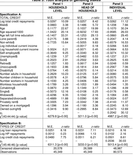
Specification A of Table 3 presents the results from the tobit analysis, where we

investigate the relationship between the amount of current credit repayments and the

amount of the gambling stakes. To evaluate the impact of a covariate on the level of

gambling expenditure, we derive the marginal effects for the censored variable from

the estimated coefficients. These are calculated by multiplying the estimated

coefficient, θ, by the scaling factor (ignoring subscripts): φ({θln(C)+π'X}/σ), where

φ denotes the cumulative distribution of the standard normal and σ is the standard

error of the regression equation.

Since monetary values are in log units, estimating the association between gambling

stakes and the amount of credit repayment is effectively evaluating an elasticity. To

be specific, a one per cent increase in credit repayments is associated with around

0.03 per cent higher total household gambling expenditure and also a 0.03 per cent

higher gambling expenditure by adult individuals. As with the probability of any

gambling, the elasticity of gambling stakes with respect to credit repayment is almost

the same for all three levels of disaggregation. In general, the factors that were seen

to determine the incidence of any gambling as reported in Table 2 are also seen to

impact upon the amount of gambling as presented in Table 3. Thus males who are

9

(17)

older, white, less educated, in work and living in public housing are more likely to

gamble, and to gamble more. Interestingly, the elasticity of gambling stakes is

equally as large in terms of magnitude as the income elasticity at the individual level.

Once again, the individual level analysis in Panel 3 allows for intra-household

correlation in gambling stakes. The correlation coefficient ρ₂ =0.2042 is positive and

statistically significant, suggesting that gambling expenditures are positively

correlated across individuals within households.

Specification B of Table 3 reports the results when credit repayments are

distinguished by type: loan repayments, HP repayments and credit club repayments.

Loan repayments dominate total credit payments as shown in Table 1. The estimated

elasticities of gambling stakes with respect to loans and, especially, credit club

payments are rather larger than for HP agreements. For example, for credit club

payments, the elasticity is about 0.05 for all three levels of aggregation (households,

heads of households and individuals), whereas for HP agreements, the elasticity is

only 0.01 for individuals and is insignificantly different from zero for households and

for heads of households.10

4. Variation in gambling and the use of credit by household income

A key question of interest is how the relationship between gambling and the use of

credit as indicators of financial risk-taking varies across household income. In

particular, do poorer households who may be more vulnerable to income uncertainty

(18)

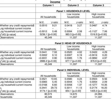
and volatility reveal rather different financial risk-taking behaviours? Tables 4 and 5

repeat the analysis in Tables 2 and 3 respectively, separately for households in the

bottom quartile and top quartile of household income. For ease of comparison, the

results for all households as obtained previously are also presented in the tables.

Only the variables of immediate interest are reported, but in each case, the other

covariates as in Table 2 and Table 3 are also included in each regression.

Table 4 reports the probit results for the incidence of any gambling and its

association with any credit repayments. The first column repeats the results from

Table 2 for all households, while the second and third columns report the results for

the low income and high income households respectively. Results are reported for

the three levels of aggregation as before in the three Panels of the table. The first

point to note is that the relationship between gambling and income is non-linear. The

overall effect measured across all households in Column 1 is estimated to be

insignificantly different from zero, but this serves to obscure an important non-linear

relationship. For low income households, there is a small but positive relationship

between household income and the probability of gambling, but for high income

households, there is a large and negative impact of increasing income on the

probability of gambling. However, the positive association between gambling and the

use of credit is approximately the same at all levels of household income, with the

use of credit associated with a 4-5% higher probability of gambling.

Similar patterns are observed for heads of households as presented in Panel 2 and

for individuals as in Panel 3, although for low income households, the positive

(19)

and not statistically significant. Individual income in high income households partly

offsets the negative relationship between higher household income and the

probability of gambling activity. The intra-household correlation (i.e. co-determination)

in gambling is stronger for low income households than for high income households.

Of most interest to this study, however, is that the positive relationship between

gambling and the use of credit is around 4-5% for all levels of aggregation and

across all household income levels. This constancy in the estimated relationship

suggests attitudes to financial risk-taking – at least with regard to the use of credit

and gambling – are rather similar across household types.

Table 5 reports the tobit results by household income. Similar patterns are observed

as in Table 4 above. The relationship between household income and gambling

stakes is non-linear, and is positive for low income households (so gambling is a

normal good) but negative for high income households (so gambling is an inferior

good). But the elasticity of gambling stakes with respect to credit repayments is

significantly positive and equal to 0.03 irrespective of household income. For heads

of households (Panel 2), and all individuals (Panel 3), similar findings are apparent,

with gambling highly inferior in high income households. Once again, there is a

stronger co-determination of the amount that individuals gamble in low income

households as compared to high income households. However, the relationship

between gambling expenditure and credit repayment is invariant to household

income.11

(20)

The number of observations and the degree of censoring shown at the bottom of

each Panel in Table 5 indicates that high income households are larger, on average.

Moreover, a greater proportion of both heads of household and individuals in high

income households do not gamble, consistent with the strong negative income

elasticity producing a lower level of gambling in high income households.12 However,

the attitudes to financial risk-taking overall seems little different by household income

bands.

5. Discussion and Conclusions

Given the recent policy changes relating to gambling in the UK along with innovations

in the gambling industry and the underlying trends towards increased gambling

activity, it is surprising that as yet there has been relatively little detailed research

regarding gambling and its determinants in the UK. Given the existence of ‘problem’

gambling as well as financial pressures at the household level, it is not surprising that

the recent changes in gambling legislation and gambling accessibility have attracted

public debate. In order to understand the potential impact of these changes at the

individual and household level, as well as on society more generally, we need to be

better informed regarding which individuals engage in gambling, the intensity with

which they gamble and, in particular, the degree to which gambling is associated with

financial vulnerability. Our empirical findings suggest a positive association between

between low and high income households are even larger when using equivalised income to define relative household income, since the intrahousehold correlations are larger in poor households and smaller in rich households than those presented in Panel 3 in Tables 4 and 5.

(21)

the propensity to engage in gambling activity and the use of credit at both the

individual and the household level. In addition, we reveal a positive relationship

between the amount spent on gambling and the level of credit repayments.

Furthermore, we find evidence supporting a positive correlation between gambling

activity across household members thereby highlighting the possibility that financial

vulnerability may be concentrated within particular types of household.

Focussing separately on poorer and richer households, we show that the relationship

between gambling and household income is non-linear. However, the propensity of

households and individuals to engage in gambling and their willingness to expose

themselves to financial vulnerability through the use of credit appears to be little

influenced or affected by household income. While richer households may be able to

better protect themselves against financial uncertainty, those in poorer households

are less able to do so. Given the current unease amongst policy makers regarding

the levels of secured and unsecured debt at the household level, the similar attitude

to financial risk-taking in terms of their propensity to gamble for given levels of

indebtedness may be a cause for concern. It would certainly merit further

(22)

REFERENCES

Blaszczynski, A., Dumlao, V., & Lange, M. (1997). How much do you spend gambling? Ambiguities in survey questionnaire items. Journal of Gambling Studies, 13, 237-252.

Brown, S., & Taylor, K. B. (2008). Household Debt and Financial Assets: Evidence from Great Britain, Germany and the US. Journal of the Royal Statistical Society, Series A, 171(3), 615-634.

Brown, S., Garino, G., & Taylor, K. B. (2008). Mortgages and Financial Expectations: A Household Level Analysis. Southern Economic Journal, 74(3), 857-878. Clotfelter, C., & Cook, P. (1989). Selling Hope. Cambridge, MA: National Bureau for

Economic Research, Harvard University Press.

Fellner, G., & Maciejovsky, B. (2007). Risk attitude and market behaviour: Evidence from experimental asset markets. Journal of Economic Psychology, 28, 338-350.

Fisher, S. (1996). Gambling and Pathological Gambling Among Casino Patrons. Report commissioned by the British Casino Industry. Plymouth: Centre for Research into the Social Impact of Gambling: University of Plymouth. Gambling Commission (2008). Gambling Industry Statistics 2007/08, July.

GamCare (2003). GamCare Care Services Report. London: National Association for Gambling Care, Educational Resources and Training.

Gropp, R., Scholz, J.K., & White, M.J. (1997). Personal Bankruptcy and Credit Supply and Demand. Quarterly Journal of Economics, 112, 217-51.

Grun, L., & McKeigue, P. (2000). Prevalence of Excessive Gambling before and after the Introduction of a National Lottery in the United Kingdom: Another Example of the Single Distribution Theory. Addiction, 95, 959-966.

Haisley, E., Mostafa, R., & Loewenstein, G. (2008). Myopic Risk-Seeking: The Impact of Narrow Decision Bracketing on Lottery Play. Journal of Risk and Uncertainty, 37, 57-75.

Ida, T., & Goto, R. (2009). Interdependency among addictive behaviours and

time/risk preferences: Discrete choice model analysis of smoking, drinking and gambling. Journal of Economic Psychology, 30, 608-621.

Lesieur, H. R. (1998). Costs and Treatment of Pathological Gambling. Annals of the American Academy of Political and Social Science, 556: 153-171.

May, O., Tudela, M., & Young, G. (2004). British Household Indebtedness and Financial Stress: A Household Level Picture. Bank of England Quarterly Bulletin, Winter, 2004.

National Gambling Impact Study Commission (1999). Final Report. Washington, DC: Government Printing Office. http://govinfo.library.unt/ngisc/index.html. Accessed 18 May 2009.

(23)

Office for National Statistics and Department for Environment, Food and Rural Affairs, Expenditure and Food Survey, 2007 [computer file]. Colchester, Essex: UK Data Archive, Various.

Shepherd, R., Ghodse, H., & London, M. (1998). A Pilot Study Examining Gambling Behaviour Before and After the Launch of the National Lottery and Scratch Cards in the UK. Addiction Research, 6, 5-12.

Sproston, K., Erens, B., & Orford, J. (2000). Gambling Behaviour in Britain: Results from the British Gambling Prevalence Survey. London: National Centre for Social Research.

Stinchfield, R., & Winters, K.C. (1998). Gambling and Problem Gambling among Youths. Annals of the American Academy of Political and Social Science, 556: 172-185.

Tokunaga, H. (1993). The use and abuse of consumer credit: application of

psychological theory and research. Journal of Economic Psychology, 14, 285-316.

Wardle H., Sproston, K., Orford, J., Erens, B., Griffiths, M., Constantine, R., & Pigott, S. (2007). British Gambling Prevalence Survey 2007. London: National Centre for Social Research, September.

Wärneryd, K-E. (1996). Risk attitudes and risky behaviour. Journal of Economic Psychology, 17, 749-770.

(24)

Table 1: Summary Statistics

Panel 1 Panel 2 Panel 3

Variable description HOUSEHOLD LEVEL HEAD OF HOUSEHOLD INDIVIDUAL LEVEL

DEPENDENT VARIABLES Mean sd Mean sd Mean sd

Whether any gambling expenditure 0.54 0.50 0.41 0.49 0.39 0.49

Gambling stakes (£) 3.59 14.78 2.22 13.63 1.96 10.71

INDEPENDENT VARIABLES

Whether any credit repayments 0.37 0.48 0.29 0.45 0.24 0.42

Whether any loan repayments 0.29 0.45 0.23 0.42 0.18 0.38

Whether any HP repayments 0.08 0.28 0.06 0.24 0.05 0.22

Whether any credit club repayments 0.05 0.23 0.03 0.17 0.03 0.17

Total payments (£) 18.45 43.62 13.10 37.62 10.24 31.48

Loan payments (£) 14.49 33.35 10.50 27.74 8.04 23.99

HP payments (£) 2.45 24.24 1.74 22.95 1.36 17.75

Credit club payments (£) 1.51 11.98 0.86 9.89 0.83 8.90

Male 0.62 0.48 0.62 0.48 0.47 0.50

Age 51.37 16.66 51.37 16.66 47.83 17.43

Age2/1000 2.92 1.78 2.92 1.78 2.59 1.75

Age left FTE 16.98 3.77 16.98 3.77 16.96 4.14

Lone-parent 0.07 0.25 0.07 0.25 0.04 0.19

White (base: omitted category) 0.94 0.23 0.94 0.23 0.94 0.24

Non-white 0.06 0.23 0.06 0.23 0.06 0.24

Log(individual income) (£) – – 10.04 1.67 9.51 2.24

Log(household income) (£) 10.52 1.18 10.52 1.18 10.69 1.12

Employee (base: omitted category) 0.51 0.50 0.51 0.50 0.52 0.50

Self-employed 0.08 0.27 0.08 0.27 0.07 0.25

Unemployed 0.02 0.14 0.02 0.14 0.03 0.16

Sick 0.06 0.24 0.06 0.24 0.06 0.23

Retired 0.27 0.44 0.27 0.44 0.23 0.42

Unoccupied 0.06 0.24 0.06 0.24 0.10 0.30

Disability 0.06 0.23 0.06 0.23 0.05 0.22

Number of adults in household 1.80 0.73 1.80 0.73 2.10 0.85

Number of children household 0.59 1.00 0.59 1.00 0.64 1.02

Number of workers in household 1.09 1.00 1.09 1.00 1.33 1.10

Workless household 0.36 0.48 0.36 0.48 0.29 0.45

Married (base: omitted category) 0.51 0.50 0.51 0.50 0.57 0.50

Cohabiting 0.09 0.29 0.09 0.29 0.10 0.30

Single 0.15 0.35 0.15 0.35 0.18 0.38

Widowed 0.12 0.33 0.12 0.33 0.07 0.26

Separated/divorced 0.14 0.34 0.14 0.34 0.08 0.27

LA/HA (base: omitted category) 0.19 0.39 0.19 0.39 0.16 0.37

Privately rented 0.09 0.28 0.09 0.28 0.09 0.28

Owned on a mortgage 0.40 0.49 0.40 0.49 0.44 0.50

Owned outright 0.32 0.47 0.32 0.47 0.31 0.46

Observations 45,349 45,349 80,573

(25)

[image:25.612.75.544.73.616.2]

24 Table 2: Probit analysis of the probability of gambling

HOUSEHOLD LEVEL

HEAD OF HOUSEHOLD

INDIVIDUAL LEVEL Specification A

TOTAL CREDIT M.E. z-ratio M.E. z-ratio M.E. z-ratio Whether any credit repayments$ 0.0510 9.21 0.0441 7.93 0.0521 10.65

Male$ 0.0148 2.48 0.0238 4.11 0.0211 5.30

Age 0.0240 20.86 0.0216 18.98 0.0251 28.20

Age squared/1000 –0.2133 18.55 –0.1934 17.07 -0.2258 24.39 Age left full time education –0.0270 29.65 –0.0251 27.34 -0.0197 27.76 Lone parent$ 0.0574 4.82 0.0532 4.45 0.0513 4.16 Non-white$ –0.1652 14.03 –0.1030 8.98 -0.1487 15.08 Log individual current income – – 0.0002 0.10 0.0065 5.45 Log household current income –0.0012 0.48 –0.0031 0.90 -0.0168 6.60 Self-employed$ –0.0891 9.49 –0.0779 8.66 -0.0835 10.48 Unemployed$ –0.0282 1.35 –0.0100 0.49 -0.0253 1.79

Sick$ –0.0470 2.82 –0.0562 3.58 -0.0649 5.71

Retired$ 0.0224 1.48 0.0117 0.80 0.0057 0.53

Unoccupied$ –0.0419 2.65 –0.0417 2.71 -0.0626 6.84 Disability$ 0.0117 0.98 –0.0069 0.60 0.0000 0.00 Number adults in household 0.0532 8.79 –0.0031 0.53 -0.0012 0.28 Number children in household –0.0135 4.41 –0.0176 5.84 -0.0144 5.58 Number workers in household 0.0348 6.05 0.0103 1.87 0.0188 4.10 Workless household$ –0.0174 1.34 –0.0177 1.42 -0.0093 1.00

Cohabiting$ 0.0067 0.70 0.0240 2.57 0.0274 3.50

Single$ –0.1086 10.96 –0.0045 0.46 -0.0055 0.74

Widowed$ –0.0924 8.41 0.0214 2.00 0.0282 2.93

Separated/divorced$ –0.1067 10.78 0.0089 0.93 0.0029 0.34 Privately rent$ –0.0635 5.99 –0.0713 7.01 -0.0991 10.81 Owned on a mortgage$ –0.0215 2.62 –0.0243 3.08 -0.0539 7.66 Owned outright$ –0.0660 8.20 –0.0615 8.01 -0.0812 11.62

ρ1 – – – – 0.2441 29.73

χ2

(43:44:44) [p value] 5236.1 [p=0.00] 2886.2 [p=0.00] 4174.1 [p=0.00]

Specification B:

TYPES OF CREDIT M.E. z-ratio M.E. z-ratio M.E. z-ratio Whether any loan repayments$ 0.0430 7.41 0.0398 6.72 0.0417 7.76 Whether any HP repayments$ 0.0014 0.16 0.0089 0.91 0.0166 1.84 Whether any credit club rep’s$ 0.0846 7.69 0.0821 5.76 0.0949 8.23

ρ1 – – – – 0.2435 29.64

χ2_{(45:46:46) [p value]} _{5271.6 [p=0.00]} _{2905.1 [p=0.00]} _{4194.6 [p=0.00]}

(26)

25

Notes to Table 2:

1. Coefficients reported are marginal effects (M.E.) on the probability that the household (Panel 1), head of household (Panel 2) or adult individuals within the household (Panel 3) engages in any form of gambling activity. For dummy variables, denoted $, the coefficient reported is for the discrete change of the dummy from 0 to 1. The ‘z-ratio’ reports the test that the underlying coefficient is equal to zero.

2. In the household level equation (Panel 1), the individual characteristics are those of the head of household. Reference categories are: female; head of household white; employee; no disability; at least one adult in work; married; local authority or housing association.

3. In Panel 3, ρ1 is the proportion of the total variance accounted for by the intra-household

variation in gambling propensity.

4. The χ2 test is a test for the joint significance of the explanatory variables.

5. The regression in Specification B which differentiates between different types of credit also includes all of the other independent variables reported in Specification A. Their coefficient estimates are little different from those in Specification A and so are not reported here but are available on request.

(27)

[image:27.612.75.543.79.621.2]

26 Table 3: Tobit analysis of gambling stakes

HOUSEHOLD LEVEL

HEAD OF HOUSEHOLD

INDIVIDUAL LEVEL Specification A:

TOTAL CREDIT M.E. z-ratio M.E. z-ratio M.E. z-ratio Log total credit repayments 0.0297 10.09 0.0257 8.42 0.0262 11.12

Male$ 0.0883 3.38 0.1486 5.72 0.1208 7.66

Age 0.1177 22.67 0.1037 19.99 0.1070 30.24

Age squared/1000 –1.0422 20.14 –0.9232 17.93 –0.9585 26.03 Age left full time education –0.1407 33.31 –0.1253 29.13 –0.0860 29.45 Lone parent$ 0.2175 3.88 0.2419 4.39 0.2047 4.14 Non-white$ –0.7725 15.64 –0.5055 9.83 –0.6579 16.53 Log individual current income – – –0.0017 0.18 0.0266 5.63 Log household current income 0.0024 0.21 –0.0071 0.45 –0.0664 6.53 Self-employed$ –0.3649 9.25 –0.3340 8.32 –0.3274 10.32 Unemployed$ –0.1239 1.37 –0.0482 0.53 –0.1237 2.21

Sick$ –0.2023 2.91 –0.2502 3.63 –0.2625 5.93

Retired$ 0.1257 1.93 0.0617 0.94 0.0248 0.59

Unoccupied$ –0.1933 2.86 –0.1814 2.64 –0.2567 7.06 Disability$ 0.0764 1.45 –0.0070 0.14 0.0214 0.55 Number adults in household 0.2629 10.23 –0.0125 0.47 –0.0080 0.45 Number children in household –0.0578 4.31 –0.0796 5.84 –0.0575 5.55 Number workers in household 0.1030 4.25 0.0406 1.66 0.0733 4.01 Workless household$ –0.1789 3.26 –0.1053 1.89 –0.0494 1.35

Cohabiting$ 0.0870 2.09 0.1349 3.17 0.1286 4.09

Single$ –0.5073 12.16 –0.0108 0.25 –0.0176 0.58

Widowed$ –0.4296 9.35 0.1042 2.16 0.1084 2.85

Separated/divorced$ –0.4889 11.88 0.0390 0.90 –0.0024 0.07 Privately rent$ –0.3305 7.23 –0.3342 7.38 –0.4143 11.37 Owned on a mortgage$ –0.1396 3.94 –0.1180 3.36 –0.2245 8.10 Owned outright$ –0.3416 9.90 –0.2995 8.84 –0.3473 12.69

ρ2 – – – – 0.2042 30.12

χ2

(43:44:44) [p value] 6279.8 [p=0.00] 3211.0 [p=0.00] 4987.2 [p=0.00]

Specification B:

TYPES OF CREDIT M.E. z-ratio M.E. z-ratio M.E. z-ratio Log loan repayments 0.0251 8.18 0.0231 7.11 0.0210 8.16 Log HP repayments 0.0012 0.23 0.0066 1.13 0.0102 2.16 Log credit club repayments 0.0480 7.75 0.0511 6.21 0.0501 8.61

ρ2 – – – – 0.2036 30.03

χ2_{(45:46:46) [p value]} _{6311.3 [p=0.00]} _{3233.0 [p=0.00]} _{5013.4 [p=0.00]}

Censored observations 20,578 26,589 48,987

(28)

27

1. Coefficients reported are marginal effects (M.E.) on the gambling stakes of the household (Panel 1), head of household (Panel 2) or adult individuals within the household (Panel 3). For dummy variables, denoted $, the coefficient reported is for the discrete change of the dummy from 0 to 1. The ‘z-ratio’ reports the test that the underlying coefficient is equal to zero.

variation in gambling stakes.

5. The regression in Specification B which differentiates between different types of credit also includes all of the other independent variables reported in Specification A. Their coefficient estimates are little different from those in Specification A, and so are not reported here but are available on request.

(29)

[image:29.612.76.543.84.497.2]

28 Table 4: Probit analysis of the probability of gambling by household

income

Column 1 Column 2 Column 3

Panel 1: HOUSEHOLD LEVEL

All households

Low income households

High income households

M.E. z-ratio M.E. z-ratio M.E. z-ratio Whether any credit repayments$ 0.0510 9.21 0.0418 3.27 0.0487 4.74

Log individual current income – – – – – –

Log household current income –0.0012 0.48 0.0094 2.58 –0.1127 7.06 χ2_{(43) [p value]} _{5236.1 [p=0.00]} _{983.3 [p=0.00]} _{1516.9 [p=0.00]}

Observations 45,349 11,337 11,337

Panel 2: HEAD OF HOUSEHOLD

All households

High income households Whether any credit repayments$ 0.0441 7.93 0.0520 4.02 0.0422 4.29 Log individual current income 0.0002 0.10 0.0007 0.19 –0.0016 0.20 Log household current income –0.0031 0.90 0.0085 1.76 –0.0892 4.97 χ2_{(44) [p value]} _{2886.2 [p=0.00]} _{677.7 [p=0.00]} _{876.8 [p=0.00]}

Observations 45,349 11,337 11,337

Panel 3: INDIVIDUAL LEVEL

All households

High income households Whether any credit repayments$ 0.0521 10.65 0.0580 4.24 0.0503 6.56 Log individual current income 0.0065 5.45 0.0044 1.75 0.0054 2.09 Log household current income –0.0168 6.60 0.0058 1.37 –0.1277 10.35

ρ1 0.2441 29.73 0.3011 11.13 0.2174 16.20

χ2_{(44) [p value]} _{4174.1 [p=0.00]} _{654.1 [p=0.00]} _{1405.0 [p=0.00]}

Observations 80,573 14,670 24,994

Households 45,349 11,337 11,337

1. Coefficients reported are marginal effects (M.E.) on the probability that the household (Panel 1), head of household (Panel 2) or adult individuals within the household (Panel 3) engages in any form of gambling activity. For dummy variables, denoted $, the coefficient reported is for the discrete change of the dummy from 0 to 1. The ‘z-ratio’ reports the test that the underlying coefficient is equal to zero.

variation in gambling propensity.

5. All regressions also include the control variable reported in Table 2, plus 6 calendar year dummy variables and 12 regional dummy variables.

(30)

[image:30.612.74.540.69.520.2]

29 Table 5: Tobit analysis of gambling stakes by household income

Column 1 Column 2 Column 3

Panel 1: HOUSEHOLD LEVEL

All households

High income households

M.E. z-ratio M.E. z-ratio M.E. z-ratio Whether any credit repayments$ 0.0297 10.09 0.0284 3.92 0.0277 5.29

Log individual current income – – – – – –

Log household current income 0.0024 0.21 0.0384 2.42 –0.5244 7.27 χ2

(43) [p value] 6279.8 [p=0.00] 1125.9 [p=0.00] 1780.2 [p=0.00]

Observations 45,349 11,337 11,337

Panel 2: HEAD OF HOUSEHOLD

All households

High income households Whether any credit repayments$ 0.0257 8.42 0.0340 4.51 0.0230 4.31 Log individual current income –0.0017 0.18 0.0004 0.02 –0.0070 0.18 Log household current income –0.0071 0.45 0.0396 1.83 –0.4169 4.96 χ2_{(44) [p value]} _{3211.0 [p=0.00]} _{752.8 [p=0.00]} _{939.4 [p=0.00]}

Observations 45,349 11,337 11,337

Panel 3: INDIVIDUAL LEVEL

All households

High income households Whether any credit repayments$ 0.0262 11.12 0.0314 4.71 0.0253 6.66 Log individual current income 0.0266 5.63 0.0156 1.66 0.0234 2.11 Log household current income –0.0664 6.53 0.0211 1.33 –0.5549 10.55

ρ2 0.2042 30.12 0.2476 11.21 0.1907 16.56

χ2_{(44) [p value]} _{4987.2 [p=0.00]} _{908.0 [p=0.00]} _{1600.9 [p=0.00]}

Observations 80,573 14,670 24,994

Households 45,349 11,337 11,337

1. Coefficients reported are marginal effects (M.E.) on the gambling stakes of the household (Panel 1), head of household (Panel 2) or adult individuals within the household (Panel 3). For dummy variables, denoted $, the coefficient reported is for the discrete change of the dummy from 0 to 1. The ‘z-ratio’ reports the test that the underlying coefficient is equal to zero.

2. In the household level equation (Panel 1), the individual characteristics are those of the head of household.

variation in gambling stakes.

5. All regressions also include the control variable reported in Table 2, plus 6 calendar year dummy variables and 12 regional dummy variables.