White Rose Research Online
[email protected]
Universities of Leeds, Sheffield and York
http://eprints.whiterose.ac.uk/
White Rose Research Online URL for this paper:
http://eprints.whiterose.ac.uk/76566/
Paper:
Li, K, Jackson, A and Livermore, PW (2011)
Variational data assimilation for the
initial-value dynamo problem.
Physical Review E - Statistical, Nonlinear, and Soft
Matter Physics, 84 (5). ARTN 056321.
Variational data assimilation for the initial-value dynamo problem
Kuan Li and Andrew Jackson
Institute of Geophysics, ETH Zurich, CH-8092 Zurich, Switzerland
Philip W. Livermore
School of Earth and Environment, Leeds University, Leeds, GB-LS2 9JT, United Kingdom
(Received 24 April 2011; revised manuscript received 16 August 2011; published 23 November 2011)
The secular variation of the geomagnetic field as observed at the Earth’s surface results from the complex magnetohydrodynamics taking place in the fluid core of the Earth. One way to analyze this system is to use the data in concert with an underlying dynamical model of the system through the technique of variational data assimilation, in much the same way as is employed in meteorology and oceanography. The aim is to discover an optimal initial condition that leads to a trajectory of the system in agreement with observations. Taking the Earth’s core to be an electrically conducting fluid sphere in which convection takes place, we develop the continuous adjoint forms of the magnetohydrodynamic equations that govern the dynamical system together with the corresponding numerical algorithms appropriate for a fully spectral method. These adjoint equations enable a computationally fast iterative improvement of the initial condition that determines the system evolution. The initial condition depends on the three dimensional form of quantities such as the magnetic field in the entire sphere. For the magnetic field, conservation of the divergence-free condition for the adjoint magnetic field requires the introduction of an adjoint pressure term satisfying a zero boundary condition. We thus find that solving the forward and adjoint dynamo system requires different numerical algorithms. In this paper, an efficient algorithm for numerically solving this problem is developed and tested for two illustrative problems in a whole sphere: one is a kinematic problem with prescribed velocity field, and the second is associated with the Hall-effect dynamo, exhibiting considerable nonlinearity. The algorithm exhibits reliable numerical accuracy and stability. Using both the analytical and the numerical techniques of this paper, the adjoint dynamo system can be solved directly with the same order of computational complexity as that required to solve the forward problem. These numerical techniques form a foundation for ultimate application to observations of the geomagnetic field over the time scale of centuries.
DOI:10.1103/PhysRevE.84.056321 PACS number(s): 47.65.−d, 05.45.−a, 41.20.−q
I. INTRODUCTION
In 1919, the British scientist Larmor first proposed that the magnetic fields of the Sun and Earth are generated and sustained by a complex and nonlinear magnetohydrodynam-ical (MHD) process [1], known as dynamo action. In the Earth’s dynamo system, the magnetic field is generated by, for example, a buoyancy-driven convecting flow of molten iron, confined to the spherical shell between the Earth’s inner core and overlying solid mantle. In order for the geomagnetic field to be sustained, the amplifying influence of induction due to the electrically conducting flow must overcome the natural tendency of the magnetic field to decay (e.g., [2]). In general, the magnetic field reacts back on the convecting iron through the Lorentz force resulting in a highly complex nonlinear system.
In order to understand more aspects of the Earth’s dynamo system, such as the spatial distributions of the velocity, mag-netic, and temperature fields [3], the convection pattern [4], possible MHD wave propagation in the core [5], and magnetic secular variation, more studies from different perspectives are required, for instance, by tackling the inverse problem. The Earth’s dynamo system continuously creates a magnetic field, which is recorded in rocks, lavas, and sediments and also observed by observatories and satellites. These observations are represented by two models: gufm1 (for the past 400 years) [6] and cals7k (for past 7000 years) [7]. For Earth, the electrical conductivity of the mantle is several orders of
magnitude weaker than that of the core; hence Earth’s mantle is assumed as an insulator and thus, the surface observed data represented bygufm1andcals7kcan be downward projected onto the core mantle boundary (CMB). Continuous data in time of the radial component of the magnetic field at the CMB are thus given as a function of spherical harmonic degreeland order m, where l13 [8]. These data provide information on the dynamo system and help to infer the inner working of Earth’s core. Notice that the magnetic field is divergence-free and Earth’s mantle is assumed as an insulator, thus a scalar observation in the radial direction is equivalent to observation of the magnetic field in all three directions at the CMB.
using observations necessarily earlier than the present, is then evolved into the future, generating predictions of the future state of the atmosphere, the weather forecast.
Despite the wide application of variational data assimilation in other fields of Earth science, its application to Earth’s dynamo system only recently began [13]. In this landmark paper [13], the authors carried out a one-dimensional (1D) toy model study as a proof of the possibility of applying a discrete variational method to the MHD system. This work was further advanced by Canet et al. [14], who developed a variational formalism for a specific dynamical model of the core, the quasigeostrophic model. This work focuses on short time scale dynamics, and thus approximates the core as a perfect electrical conductor; is has been the basis for the recent remarkable discovery of torsional oscillations in the core with time scales on the order of six years [15]. The common thread to these works is the setting of the problem in a discrete form and the derivation of the adjoint system under this discrete form. Because of the large storage requirement and heavy computational burden in solving the discrete adjoint nonlinear problem [13], it is our purpose to develop the adjoint dynamo system in terms of continuous functions and also design the corresponding algorithms, which carry out the computation of the adjoint model more efficiently.
An allied, equally influential strand of data assimilation has been developed in a geomagnetic context in parallel with the variational approach, based on sequential data assimilation (see, e.g., [16]). This effort began with the work of Sun
et al.[17] and Liuet al.[18] and has been recently reviewed in Fournieret al. [19] and Kuang and Tangborn [20]. This approach is based on the use of classical sequential data assim-ilation methods being applied to a geodynamo model [21] to create a framework for guiding the trajectory via observational constraints [22,23]. The results are so encouraging that the approach has culminated in a sequential data assimilation model [24] contributing to the predicted secular variation of the most recent International Geomagnetic Reference Field [25].
A criterion must be introduced measuring the agreement between physical observations and predictions of the model. There is considerable flexibility in the way this agreement is measured [e.g., [10,26] but a very convenient measure is based on a weighted squared deviation, often termed
χ2. Regardless of the definition of goodness of fit between the observations and the model prediction, the process of estimating the parameters governing a dynamical system by taking into account observations is usually termed data assimilation(4Dvar).
The functionalχ2is called the misfit and the optimal predic-tion occurs at the global minimum ofχ2; finding this minimum is, in general, a nonlinear process. Generally speaking, the adjoint assimilation relies on deriving the adjoint system of the forward model, which is, mathematically speaking, the total derivative of χ2 with respect to the unknowns constrained by the forward model. The adjoint model is driven by the combination of observations and predictions backward in time, and its value at the initial time is the downhill direction of the misfit with respect to the unknown control parameters which define the initial condition. The current values of the unknown control parameters are updated recursively in this downhill direction. Hence, a most important aspect of
the analysis involves deriving and computing the adjoint model.
The format of the paper is as follows. In Sec. II, we discuss the fundamental mathematics, including the general mathematical framework of the adjoint method for the initial-value problem, the choice of the boundary condition of the adjoint field, and the matrix representation of the linear operator and its adjoint. SectionIIIdescribes the applications to a kinematic dynamo and to an illustrative Hall-effect nonlinear problem, from which we understand the adjoint form of the divergence-free equation of magnetic induction; we also develop the proper numerical algorithm for computing the adjoint system. Some numerical results are reported in Sec.IV. Based on these results, we derive the adjoint system of the dynamo problem in Sec.V. Finally, in Sec.VI, we draw conclusions and discuss the outlook for further work.
II. MEASUREMENTS AND AN UNDERLYING DYNAMICAL MODEL
A. Geomagnetic data
Variations of the magnetic field have been recorded either by direct human observation for the last few hundred years [6] or through the magnetization of rocks and artifacts over the last few thousand years [7]. These observations have sensitivity to the magnetic field originating in the core of the Earth. We adopt the standard approximation of assuming the mantle to be an electrical insulator. Then the vector observations of the magnetic field at the Earth’s surface B
are related to the radial component of the magnetic field at the core surface through a Green’s function appropriate for the solution of Laplace’s equation in a spherical geometry, subject to Neumann boundary conditions [27,28]. The ill-posedness of this problem is clearly understood, and its remedies through the technique of regularization [e.g., [29] are routinely implemented. Geomagnetic data are inherently imperfect measurements and are subject to the presence of noise. Thus one normally chooses to fit the data under a least-squares criterion where each datum is weighted inversely by its estimated error.
For the purposes of our study we do not deal with the intricacies of dealing with real data; instead we assume this problem has been solved and that what is available is the spherical harmonic expansion of the radial magnetic fieldBr at the core-mantle boundary, or equivalently the values of the spectral components of the poloidal scalar on the core surface [see Eq. (14)]. This shortcut of sidestepping the difficulties attendant to real data is in accord with the previous initial work of others [e.g., [22]].
B. The variational data assimilation method for initial-value problems
Consider a time-evolving physical system given by the following governing equation:
∂
∂tP=X(P), (1)
a spatial operator. Depending on the physical system,X(•) could be a linear or a nonlinear operator acting on a target field •. Thus in the examples detailed in this paper, for a diffusion process, X is a linear operator, namely, ∇2•; for a kinematic dynamo, X is a linear operator given by ∇×(u× •)+∇2•, where u is the velocity of the flow; and for a Hall-effect problem, X is nonlinear given by ∇×[(u+∇× •)× •]+∇2•.
The dynamical system is defined in the volumeV and time interval τ. The vector P is a function of the locationr and timetand is uniquely determined by the initial and boundary conditions. Without losing generality, we assume the scalar square integrable functiony(r,t) is a measured property of the dynamical system.
Our aim is to find the predictions fromP(r,t) that agree best with the observed datay. First, we define the inner product inL2 (Lebesgue square integrable) as the integral over the volume. Forf,g∈L2, the inner product is
f,g =
V
wf g dV , (2)
where w is the integration weight, and hence we define a misfitχ2, measuring the disagreement between observations and predictions within the observation time windowt∈[0,τ], as
χ2= 1
2
V
t=τ
t=0
w[O(P)−y]2 dV dt
= 1
2
τ
t=0
O(P)−y,O(P)−ydt, (3)
where O is the observation operator, which generates the predictionO(P) at the same positions in space and time as the measurementsy(r,t).
In Eq. (3), the misfit χ2 depends purely on the initial condition, and an optimal solution (i.e., a local or global minimum) for the initial conditionP0=P(r,t=0) is given by∇P0χ
2=0, where∇
P0χ
2 is known as the gradient ofχ2
with respect to the initial conditionP0.
However, in general, it is hard to compute∇P0χ
2directly,
since P is governed by the dynamic system (1) and the associated boundary conditions. One standard approach is to introduce a Lagrange multiplierP†[16,30] and define a new constrained functional χ2 by augmenting Eq. (3) with the dynamical constraints to give
χ2= 1
2
τ
t=0
O(P)−y,O(P)−ydt
+
τ
t=0
P†,∂
∂tP−X(P)
dt. (4)
Mathematically speaking,P†is also known as the adjoint field ofP.
1. Continuous approach
The differential of a functional in a Banach space is called Gˆateaux differentiation [31] and is consequently so defined
in a Hilbert space too, e.g. L2. For example, the Gˆateaux differential ofO(P) in the direction ofqis defined as
D(O(P))=lim →0
O(P+q)−O(P)
=O(q). (5)
where D stands for Gˆateaux differentiation and in order to keep our discussion simple, we assume that the observation operatorOis linear in our paper. Notice thatqis an arbitrary direction and can be equivalently represented consideringOas the identity operator asq=lim→0 P+q−P =DP, according to the definition of Gˆateaux differential in (5). Therefore, we can writeD(O(P))=O(q)=O(DP). Differentiating the constrained misfitχ2in the directionDP, we have
Dχ2 =
τ
t=0
O(DP),O(P)−ydt
+
τ
t=0
P†,∂
∂tDP−X
(DP)dt, (6)
where X is the linearized differential of X, known as the tangent linear operator [13].
Integrating Eq. (6) by parts, we look for adjoint operators ∂
∂t and [X]†and find
Dχ2 =[DP,P†]τt=0
+
τ
t=0
DP,− ∂ ∂tP
†−[X]†(P†)+O†[O(P)−y]dt,
whereO†is the adjoint observation operator satisfying
O(DP),O(P)−y = DP,O†[O(P)−y] and [X]†is the adjoint operator ofXsatisfying
P†,X(DP) = [X]†(P†),DP.
The boundary condition onP†must be chosen; see Sec.II D. Further imposing the terminal condition thatP†=0 att =τ, we have
Dχ2 = −P†0,DP0
+
τ
t=0
DP,− ∂ ∂tP
†−[X]†(P†)+O†[O(P)−y]dt.
In a Hilbert space, Gˆateaux differentiation can be further written in the form of an inner product [31]. For example, the Gˆateaux differentiation of the misfit χ2 can be written as Dχ2= ∇
P0χ
2,DP
0. Hence the downhill direction with respect to the current prediction of the initial condition is
∇P0χ
2= −P†
0, (7)
whereP†satisfies the following adjoint system:
−∂
∂tP
†=[X]†(P†)−O†[O(P)−y]. (8)
2. Discrete approach
Let{qi}be a complete set of vectorsi→ ∞that can be used to representPin Eq. (1). The basisqi is orthogonal with an inner product 2given byqi,qj2 =
V w2qi·qjdV =δi,j, where the integration is over the volumeV andw2is a weight function.
The differential equation (1) can be approximated by a finite dimensional system and written in matrix form. And hence the forward problem (1) can be written in the spatially discretized form as
∂
∂tf=Mff, (9)
where f=[q1,P2,q2,P2, . . .]T is the discrete form of
P and the matrix Mf ([Mf]i,j = qi,Xqj2) is the matrix representation ofX. Notice that if the operatorXis nonlinear, the matrix representation of the operatorX depends on the current state off.
Guaranteed by the Riesz representation theorem, the adjoint of bounded operators, such as matrices, always uniquely exists [32]. Hence, one can approximate the adjoint tangent linear operator [X]†in Eq. (8) by their matrix representations. Let us denote the matrix representation of [X]†by, wherei,j =
qi,[X]†qj2. The adjoint system in Eqs. (7) and (8) can be written as
∇f0χ
2 = −f† 0,
(10)
−∂
∂tf
†=f†−O†(Of−y),
where f†=[q1,P†2,q2,P†2, . . .]T is the discrete form of
P†,Ois the discrete form of the observation operatorO, and
yis the set of observations.
Notice that we derive the continuous adjoint system using the inner product and we discretize the continuous system using 2. If these two inner products are identical, i.e., =
2(requiringw=w2), one can easily show
Zi,j = qi,Xqj = [X]†qi,qj =j,i (11)
by the definition of the adjoint operator, whereZis the matrix representation of the tangent linear X. Hence =Z† and furthermore, the continuous adjoint and discrete adjoint are entirely numerically equivalent.
C. Numerical approaches and their computational complexity
We have shown the equivalence of the continuous and discrete approaches in solving the adjoint system in Sec.II B 2, ifXis discretized and [X]†is derived and discretized in the same Hilbert space. It means that the adjoint operator can be treated as a black box. Instead of deriving the analytical form of the adjoint operator [X]†, one could solve the adjoint system by simply taking the transpose conjugate of the matrix representation ofX[13].
Generally speaking, ordinary differential equations (ODEs) or partial differential equations (PDEs) can be solved by the following two different approaches using spectral methods [33]: (1) a matrix-free algorithm, which requires computing the forward and inverse spectral transforms and (2) a matrix-based
algorithm, which requires computing the matrix representation of the operators in ODEs or PDEs.
Suppose we would like to evolve a three-dimensional (3D) geodynamo and its adjoint system with the spatial truncation
Nmax=Lmax=mmax=k, where Nmax,Lmax, and mmax are the maximal degree and order in the radial, colatitude, and longitude directions in spherical coordinates. Using the first method, at each time step, the spatial transform requires
εk4 operations [34,35], where ε is a prefactor. In contrast, the matrix-based algorithm requires computing the matrix representation of the spatial operators of dimension 2k2(k+2) [35]. Since the system is nonlinear, at each time step the matrix representations of the nonlinear operators have to be recomputed, and computing each column requires ε2k4 operations. Therefore, at each time step the computational complexity in computing the matrix representations is bounded by ε3k7, which is k3 slower than method (1), where ε3 is a prefactor. Typical spatial resolutions for geodynamo calculations are several hundred basis functions in each spatial direction [36]. If k=100, solving the geodynamo and its adjoint system using method (1) is 106times faster than method (2). Furthermore, the matrix dimension fork=100 resolution is about 2×10⁶ and occupies more than 20 terabytes in storage, which is extremely difficult for current computer clusters to handle. Therefore, method (2) is not directly applicable to large complex systems like the geodynamo problem. The conventional way to solve the adjoint system is to mechanically adjoint the forward code [37,38]. However, the geodynamo is a very complex system and the computer code is programed and parallelized in a sophisticated way. It would be very challenging to adjoint the dynamo codes by hand [19]. Therefore, we are interested in developing the continuous adjoint dynamo system and the corresponding numerical algorithm.
D. Updating the estimated initial condition
Having the derivative of χ2 in hand (Sec. II B), we can now optimize the initial condition, so that the fit to the data is improved. This can be carried out recursively by updating the current initial condition estimateP(n)0 using a simple descent algorithm,
P(n0+1)=P(n)0 −μ∇P(n) 0 χ
2=P(n)
0 +μP†0, (12)
whereμis the searching length andP†0 is the solution of the adjoint system (8) at thenth iteration ofP0.
1. Constraints on the adjoint fieldP†in 4Dvar
It must be noted that the boundary condition ofP† is not arbitrary. In Eq. (12), the uphill direction of the misfit is given as ∇P0χ
2= −P†
0, which leads to an update of the boundary condition of P(n)0 . Thus when deriving the adjoint system or directly computing the matrix representation of the adjoint operator, there are two principles that need to be satisfied:
(1) If the field P is a divergence-free or curl-free field, i.e., ∇·P=0 or∇×P=0, the adjoint field P† has to be divergence-free or curl-free.
forward problem. Let us use K(P)=c to represent the boundary condition ofP. For both linear homogeneous and inhomogeneous boundary conditions of P, one can have
K(P+μP†)=K(P)+μK(P†)=cfor anyμ. SinceK(P)=
c, the adjoint fieldP†has to vanish asK(P†)=0. For example, if the field ∂
∂rP+P=Hat the boundary r=1, the adjoint fieldP†has to satisfy ∂
∂rP†+P†=0 atr=1.
We use a Galerkin method in this paper (see Sec.III Aand AppendixA) in which every one of the radial basis functions satisfies the boundary conditions. This gives us the flexibility to use a more general updating scheme than Eq. (12), whereby
μin Eq. (12) is replaced by a preconditioning matrix [39].
III. DERIVATION OF ADJOINT OPERATORS FOR INDUCTIVE SYSTEMS
In this section we introduce two problems of increasing non-linearity to illustrate how the adjoint systems can be derived. We evolve magnetic fields subject to specified physical laws, and show how their initial conditions can be recovered. The first example has a linear spatial operatorX, and the second has a nonlinear operator. The motivation for these examples is the following. The example with a linear operatorX (the induction equation with a prescribed flowu) is the simplest possible physically relevant example. Despite this, it of course exhibits considerable complexity in its evolution. We devise our second problem to have nonlinear evolution, since the spatial operator in the given Hall-effect problem now depends quadratically on the magnetic field. These examples serve to illustrate the critical problems inherent in the full dynamo equations, which are ultimately tackled in Sec.V.
A. Example 1: The kinematic dynamo and its adjoint
We nondimensionalize the magnetic induction equation (e.g., [2]) by choosingUandLfor the characteristic velocity and length scales. Defining a magnetic Reynolds number,
Rm=U L/η, the induction equation including a possible
α-effect term (whereαis a mean-fieldαeffect parametrizing the interactions of the small scales) is written as [2]
∂B
∂t =Rm∇×[u×B+α(r)B]+∇
2B, (13)
whereBis the magnetic field,uis the velocity field, and the general tensorαhas been assumed to be isotropic. In our study, the kinematic dynamo is defined in a unit sphere and we assume the flow is incompressible, thus bothuandBare divergence-free and can be uniquely represented using a poloidal and toroidal decomposition. For example, in a spherical geometry with coordinates (r,θ,φ), the magnetic field can be written as
B=
(n,l,m)
a(n,l,m)nSml +b(n,l,m)nTml
,
where {a(n,l,m)} and {b(n,l,m)} are spectral coefficients, the poloidal and toroidal vectors are given by [28]
nSml =∇×∇×
l n(r)Y
m l (θ,φ)ˆr
,
(14)
nTml =∇×
l n(r)Y
m l (θ,φ)ˆr
,
and where ˆris the unit vector in ther direction;l
nand
l n are radial basis functions with degreenless than or equal to
Nmax, the radial truncation level. In colatitudeθand longitude
φ, the spherical harmonicsYlm(θ,φ) [28] that we use are real and fully normalized in solid angle and have degree l and ordermsatisfying the truncation 0mlLmax, for some specified truncation Lmax. We may further indicate either a cosine or sine azimuthal dependence of a nonaxisymmetric harmonic by the addition of either “s” or “c” as a superscript: e.g., nSmcl .
When the sphere is surrounded by an electrical insulator, the radial basis functions must obey the following boundary conditions [40]:
dln/dr+lln=0 at r=1,
(15)
nl =0 at r=1,
where the definitions of ln and nl can be found in AppendixA.
For the sake of simplicity, we initially treat the case where α=0 and use nonslip boundary conditions for u, thusu=0 atr=1. Let us denoteL1(B)=Rm∇×(u×B) andL2(B)=∇2B. Namikawa and Matsushita [41] found the adjoint kinematic dynamo system, where the inner product is defined by the energy norm, and in mathematical language the adjoint operators can be written as
L†1(B†)=Rm(∇×B†)×u and L†2(B†)=∇2B†, (16)
where the diffusion operator L2 is self-adjoint and the boundary condition for B† stays the same as that for B, namely, the electrical insulating boundary condition (15). However, of most interest is the adjoint operator L†1. Using the vector identity∇·(a×b)= −(∇×b)·a+(∇×a)·b
and integrating by parts, we have
B†,∇×(u×B) =
V
B†·[∇×(u×B)]dV
=
[(u×B)×B†]·d
+
V
B·[(∇×B†)×u]dV , (17)
where the inner product is defined in Eq. (2) with unit integration weightw=1 anddis the surface element. Since
u=0 atr=1, the surface integral vanishes, thus we have
B†,L1(B) =Rm
V
B·[(∇×B†)×u]dV = L†1(B†),B.
(18)
Notice that ∇·B=0 and ∇·L1(B)=0; hence L1 is the linear mapping from divergence-free field back to itself. Following our remarks in Sec. II D 1, the adjoint operator
L†1 has to be divergence-free for the initial-value problem. However, the adjoint term (∇×B†)×udoes not satisfy such a condition. Also notice thatBis uniquely represented by the poloidal and toroidal fields (14), hence the linear operatorL1 is densely defined inL2and its adjoint,L†
constraint, i.e.,∇·B=0 to the misfit functionalχ2in order to annihilate the non-divergence-free part. We write
χ2= 1
2
τ
t=0
O(B)−y,O(B)−ydt
+
τ
t=0
B†,
∂
∂t −L1−L2
(B)
dt
+
τ
t=0
p†,∇·Bdt,
wherep†is a new Lagrange multiplier.
Taking the Gˆateaux differentiation, integrating by parts and introducing the terminal boundary condition ofB†=0 att = τ, we have
∇B0χ
2= −B†
0,
0=
τ
t=0
DB,∂B †
∂t
dt+
τ
t=0
DB,O†[O(B)−y]dt
+
τ
t=0
DB,Rm(∇×B†)×u+∇2B†dt
+
τ
t=0
DB,−∇p†+ˆrp†δ(r−1)dt, (19)
where the derivation of the last term on the right-hand side of Eq. (19) is
∇·DB,p† =
V
(∇·DB)p†dV
= −
V
DB·∇p†dV+
V
∇·(DBp†)dV
= −
V
DB·∇p†dV+
V
DB·ˆrp†δ(r−1)dV
= DB,−∇p†+ˆrp†δ(r−1). (20) Notice that Eq. (20) is true for any arbitrary boundary condition ofp†. However, the zero boundary condition, i.e.,p†|r=1= 0 is the simplest one, since the boundary term p†DB· ˆrd= DB·ˆrp†δ(r−1)on the right-hand side of Eq. (19) vanishes, whereis the core surface. Therefore the complete form of the adjoint induction operator is
L†1(B†)=Rm(∇×B†)×u−∇p†, (21)
where the Lagrange multiplierp†plays the role of the adjoint pressure and
∇2p†=R
m∇·[(∇×B†)×u]. (22)
Therefore, the adjoint dynamo model can be written as
∇B0χ
2 = −B†
0,
−∂B†
∂t =Rm(∇×B
†)×u−∇p†+∇2B†
−O†[O(B)−y],
where the adjoint pressure term satisfies Eq. (22) with the zero boundary conditionp†|r=1=0. For a general 3D vector field, there is a subset s, where each element in s is both divergence-free and curl-free, i.e.,∇×∇×[rl+1Ym
l (θ,φ)ˆr]∈
sin spherical coordinates. Hence, the adjoint pressure together with its associated boundary condition determines how much
of the field insbelongs to the adjoint induction termL†1(B†) and how much of that needs to be removed together with the purely curl-free field from L†1(B†) in order to maintain the divergence-free condition (21). It is pertinent to note that adjoint dynamo equations were obtained by Roberts [43], Gibson and Roberts [44], and Kono and Roberts [45], but for an adjoint magnetic field in a finite conductor that obeys different boundary conditions to the original magnetic field. Thus these interesting adjoint equations cannot be applied to the problem at hand.
In some situations, the flow is assumed to be stress-free at the boundary or completely inviscid, thus the velocity field does not vanish at the boundary, and only a nonpenetration condition applies, i.e., ur =0. Thus the adjoint operator L†1 has to contain a boundary term. Converting the surface term into a flux injection term, we can rewrite the surface integral in Eq. (17) as
[(u×B)×B†]·ˆrd
=
V
B·[(u·B†)ˆr−B†ur]δ(r−1)dV
=
V
B·ˆr(u·B†)δ(r−1)dV ,
where ˆr(u·B†) is the flux injection which drives the adjoint system.
We now consider the modifications to the inductive term that are required when theα-effect term is present. The adjoint system with anαeffect can be written as
V
B†·∇×(αB)dV =
(αB×B†)·d
+
V
B·α(∇×B†)dV , (23)
where the boundary term can be further written as a flux injection term as
(αB×B†)·d=
V
B·α(B†×ˆr)δ(r−1)dV .
Hence, the adjoint operator of theα-effect term reads
L†α(B†)=Rm[α(B†×ˆr)δ(r−1)+α(∇×B†)].
Equation (23) is considerably simplified whenαis a constant: the surface term vanishes, and indeed the operator Lα is self-adjoint as we now demonstrate. Using the poloidal and toroidal decomposition, we find that the two integrals
αVB†·(∇×B)dV andαVB·∇×B†dV are nonzero, only if the following two conditions are satisfied [40]: (1)
l=landm=m, wherelandmare the spherical harmonic degree and order ofB†, andlandmare the spherical harmonic degree and order of Band (2) ifB†is poloidal,Bhas to be toroidal, and vice versa.
In summary, the complete form of the adjoint magnetic induction system reads
L†1(B†)+L†2(B†)+L†α(B†)
= −∇p†+Rm[(∇×B†)×u+α(∇×B†)]+∇2B†
+Rm[ˆr(u·B†)δ(r−1)+α(B†×ˆr)δ(r−1)],
whereLαis the linear operator for theα-effect term [2]. Having the adjoint operator of the induction equation in hand, we may write the adjoint system of Eq. (13) as follows:
∇B0χ
2 = −B†
0,
−∂B†
∂t =Rm[(∇×B
†)×u+ˆr(u·B†)δ(r−1)]+∇2
B†
+Rm[α(∇×B†)+α(B†×ˆr)δ(r−1)]−∇p†
−O†[O(B)−y], (24)
whereOstands for the observation operator,y stands for the observations, the boundary condition of B† stays the same as B, namely, an electrically insulating boundary condition (15), andp† vanishes atr=1 and satisfies∇2p†=Rm∇· [(∇×B†)×u].
B. Example 2: The Hall-effect dynamo model and its adjoint
The Hall-effect model of magnetic field evolution of a neutron star was first proposed by Jonse [46], where the nondimensionalized governing equation reads [47]
∂B
∂t =RB∇×[(u−∇×B)×B]+∇
2B. (25)
The Hall parameterRB [48] measures the ratio of the Hall-effect time scale τH = enBeR2 against the magnetic diffusion
time scaleτD=R2/η,RB = ττH
D =
B
eneμ0η in SI units, where R is the radius of the star. The whole Hall system is nondi-mensionalized usingτDfor the time scale. In the definition of
RB,Bis the typical magnetic field strength,μ0is the magnetic permeability,eis the charge of the electron,neis the electron’s number density, andηis the magnetic diffusivity. In order to focus on the Hall effect, we setu=0.
We choose a vertical boundary condition on the magnetic field, i.e.,Bθ=Bφ =0 atr =1. It can be shown that the Hall-effect term does not create or annihilate energy and the energy of the whole system in the unit sphere will monotonically decay. Integrating by parts, we have the energy of the system in the unit sphere,
1 2
d dt
V
B2dV = −
V
RBB·∇×[(∇×B)×B] (26)
−B·∇2BdV = −
V
(∇×B)2dV <0.
For this boundary condition, the radial basis functionsInl(r) andl
n(r) of the poloidal and toroidal magnetic fields have to satisfy
dIl n(r)
dr =0 and
l
n(r)=0 at r=1. (27)
In AppendixA, we define the spectral basis functionsIl n(r) and l
n(r) for the whole sphere satisfying these boundary conditions.
In light of the discussions of Sec.III A, we are in a position to quickly derive the adjoint of Eq. (25). The misfit functional
χ2 constrained by the Hall-effect model and the divergence-free condition of the magnetic field can be written as
χ2 = 1
2
τ
t=0
O(B)−y,O(B)−ydt+
τ
t=0
p†,∇·Bdt
+
τ
t=0
B†,∂B
∂t +RB∇×[(∇×B)×B]−∇
2B
dt,
where the inner product is defined as the volume integral over the unit sphere, the time integral is over the whole observation time window t ∈[0,τ], and the Lagrange multiplierp†is the adjoint pressure. Taking the total derivative ofχ2 with respect toB
0, integrating by parts and imposing the terminal condition thatB†=0 att =τ and a zero boundary condition onp†(p†|r=1=0), one finds
∇B0χ
2 = −B†
0,
0=
τ
t=0
DB,−∂B †
∂t +RB(∇×B
†)×(∇×B)
+RB∇×[B×(∇×B†)]−∇2B†+∇p†
+O†[O(B)−y]
dt+S1+S2+S3,
where the three boundary terms are
S1=RB
τ
t=0
{[(∇×DB)×B]×B†} ·ddt,
S2=RB
τ
t=0
{[B×(∇×B†)]×DB} ·ddt, (28)
S3=RB
τ
t=0
{[(∇×B)×DB]×B†} ·ddt.
The integrands of the three boundary terms are either orthogonal to B or B†, thus they do not have radial components and the boundary terms vanish. The adjoint system can be represented as
∇B0χ
2= −B†
0,
−∂B†
∂t = −RB{(∇×B
†)×(∇×B)+∇×[B×(∇×B†)]}
+∇2B†−∇p†−O†[O(B)−y], (29)
where
p†|r=1=0, ∇2p†= −R
B∇·[(∇×B†)×(∇×B)],
and the boundary condition onB†stays the same as that for
B, namely, Eq. (27).
C. Numerical method
a vertical boundary condition for the Hall-effect problem. A similar approach can be found in [35]. The Laplace operator ∇2is discretized using the same poloidal and toroidal scalars at the same resolution.
As we discussed in Sec.II B 2, if the continuous adjoint system is derived and discretized in the same Hilbert space, the continuous and discrete approaches are numerically equiv-alent. In our analysis, we derive the adjoints for the kinematic dynamo and Hall-effect problems using the energy norm. Hence if we discretize these two systems using the same energy norm, the continuous and discrete adjoint are equivalent. In a spherical geometry, the incompressible flow u can also be expanded in poloidal and toroidal fields,
u=
l,m
∇×∇× slm(r)Ylm(θ,φ)ˆr+∇× tlm(r)Ylm(θ,φ)ˆr,
whereslmandtlmare poloidal and toroidal scalars, respectively. We first check the numerical accuracy of the adjoint algorithm for computing −∇p†+(∇×B†)×u+ˆr (u·B†)δ(r−1), where the flow is incompressible and vanishes at the surface of the sphere (r=1) and we take the poloidal and toroidal scalars for the representation of the flowuas [49]
s20(r)=c2r3(1−r2)3, t10(r)=c1r2(1−r2). (30)
The coefficients are c1=8.107 929 179 422 066 and c2=
1.193 271 237 996 972 in fully normalized real spherical har-monics. We demonstrate the equivalence of the discrete and continuous approaches to this problem by computing the matrix representation M of ∇×(u×B) using the algorithm in Appendix B2a and by computing the matrix
of −∇p†+(∇×B†)×u+ˆr (u·B†)δ(r−1) using Ap-pendixB2b, where analytically=M†. Notice that the flow is axisymmetric, thusMandare block diagonal with each block representing a different spectral orderm. We compute the largest numerical error of each nonzero entry ofM†and
, where the relative error is E=max|Mj,i−i,j
Mj,i |. For the
highest resolutions tested,Nmax=Lmax=30 andm=0, the numerical algorithm exhibits machine precision, namely, the relative error E is found to be less than 10−13. Notice that the spectral transform in theφdirection is carried out via fast Fourier transform using FFTW [50], which is a well known stable and fast algorithm, thus there is no need to test the nonaxisymmetric modes other thanm=0.
The time stepping is carried out via a Crank-Nicolson scheme, where the diffusion term is treated implicitly and the magnetic induction and Hall-effect terms are treated explicitly for both forward and adjoint problems. For example, the induction equation in time is discretized as
Bi+1=
1−t
2 ∇
2
−1
×
Bi+t Rm∇×(u×Bi)+
t
2 ∇
2B i
.
The minimization of the misfit is carried out using a limited memory quasi-Newton method (L-BFGS). Approximating the misfitχ2up to the quadratic term, we have
χ2(P0+P0)≈χ2(P0)+∇P0χ
2(P
0)·P0 +β12P0·H·P0,
where H is known as the Hessian and the parameter β is chosen to satisfy the Wolfe conditions [39]. Then the Newton stepP0satisfies
∇P0χ
2(P
0+P0)=∇P0χ
2(P
0)+βH·P0=0. (31)
Hence the improvement of the initial condition is P0=
−βH−1∇P0χ
2(P
0), where the inverse Hessian H−1 is esti-mated and gradually improved in the minimization step. In our numerical study, we have not directed much effort to the optimal choice of parameters (e.g., β) in Eq. (31). We simply use the algorithm to demonstrate gradual improvement of the estimation of the initial condition. Our Galerkin method ensures that the correct boundary conditions are always adhered to. The numerical algorithm is based on Nocedal [51] and the software package is acquired from [52].
IV. VALIDATION OF THE ADJOINT SYSTEMS
A. Synthetic data generation
In the following examples we demonstrate the ability of our algorithms to correctly recover the initial conditions of some physical systems. To do so we generate synthetic data under two scenarios. In the first, which we refer to as two-dimensional (2D) observations, we generate data corresponding to the value of the spectral coefficients of the poloidal scalarSml on the core surface for all degrees and orders of spherical harmonic up to the model resolution at regular time intervals. This corresponds exactly to the real-life situation of boundary value observations. In the second scenario we supply values of the spectral coefficients of the poloidal scalarnSml at regular time intervals. This corresponds to full knowledge of the poloidal field within the core (hence we term this 3D observations), but there is no information concerning the toroidal field. We use this test to discover whether we have sufficient sensitivity to find the toroidal field in the core.
We perform the closed-loop testing by first defining the true initial condition of the kinematic dynamo and Hall-effect system. Starting from the truth, the dynamical system generates a trajectoryB(B0,t) in phase space, whereB0is the initial condition ofB. Although we carry out our computations in terms of nondimensionalized variables, we will report our results here in dimensional units (years), pertinent to the Earth. The conversion requires specification of the magnetic diffusivity and size of the conducting core; we take η=
1.5 m2 s−1 andr=3500 km. The lowest decay modes for a core with insulating or vertical boundary conditions have eigenvaluesλ=π2andλ=7.5, respectively; the correspond-ing decay times ληr2 are 26 000 and 34 000 years. Neglecting this difference of 30%, we take the decay time of the slowest mode to be 30 000 years in both cases. We choose different combinations of observation time and different observation techniques for study, where the observation time window is either 7000 years or 30 000 years and the observation technique is either 2D or 3D. We define the discrete misfit as
χ2=1
2
i
[O·ai−yi]T ·[O·ai−yi], (32)
timeti,yiis the list of observations atti, andOis the discretized observation operator.O splits in the spherical degree l and
mand hence is a block-diagonal matrix for both scenarios. For 2D observations, each diagonal matrix is actually a row vector,Ol,m=[l(l+1)
l
1
r2 ,
l(l+1)l
2
r2 , . . . ,
l(l+1)l n
r2 ]r=1, and for 3D observations, each Ol,m is also a diagonal matrix, Ol,m= diag[l
1,l2, . . . ,ln]r=1, wherelnis the poloidal radial basis.
B. Example 1—Kinematic dynamo numerical results
We choose Eq. (30) as the velocity of the kinematic dynamo. Notice the flow is axisymmetric, thus the magnetic field decouples in spherical harmonic orderm. When solving axisymmetric induction problems, the spatial computation complexity increases as the cube of the spatial resolution. For fully 3D problems, the computational complexity scales as spatial resolution to the power of 4 [35]. Furthermore, the time step is a decreasing function of spatial degree, max[Nmax,Lmax]. We set the true initial condition ofBto be
a(1,1,1c/s)=1 andb(1,1,1c/s)=1, wherea(n,l,mc/s)andb(n,l,mc/s)
are poloidal and toroidal coefficients, and set the starting estimate of the initial condition to be B(0)0 =0. Limited by single CPU computing power, we choose the spatial resolution for the kinematic dynamo to be Nmax=Lmax=15 for the
m=1 component (since the solution is entirelym=1) and the magnetic Reynolds number to beRm=50. The optimal time step is about 10−4, found experimentally.
We observe the radial component of the magnetic field everywhere exactly on the CMB (r=1) for each spherical harmonic degree l and order mup to the model resolution every 100 years for 30 000 years.
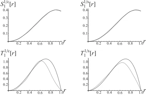
The initial condition of the magnetic field can be retrieved well. Figure 1 illustrates the true initial condition (dashed black) and the rebuilt initial condition (solid gray) of the magnetic field at the 500th iteration. The misfit drops by 11 orders of magnitude in 500 iterations (Fig.2), whereχ2 is renormalized by its value at the first iteration. Notice that there is no information concerning the toroidal field in the observed
0.2 0.4 0.6 0.8 1.0r 0.1
0.2 0.3 0.4
S11 cr
0.2 0.4 0.6 0.8 1.0r 0.1
0.2 0.3 0.4
S11 sr
0.2 0.4 0.6 0.8 1.0r 0.2
0.4 0.6 0.8 1.0
T11 cr
0.2 0.4 0.6 0.8 1.0r 0.2
0.4 0.6 0.8 1.0
[image:10.608.314.555.71.234.2]T11 sr
FIG. 1. The test case of a kinematic dynamo forRm=Rm =50:
the true versus the rebuilt initial condition for an axisymmetric kinematic dynamo represented by the poloidal and toroidal radial scalars of them=1 component, where the dashed black lines stand for the true initial condition and the solid gray lines stand for the rebuilt initial condition after 500 iterations.
100 200 300 400 500
N
109
107
105
0.001 0.1
[image:10.608.56.292.526.684.2]χ
2FIG. 2. For the test case of a kinematic dynamo problem for Rm=Rm=50, the reduction of the misfit χ2 as a function of the
number of iterationsN, whereχ2is normalized by its value atχ2of
the first iteration.
data. The toroidal field is retrieved, due to the inductive coupling [40], where the poloidal velocity interacts with the toroidal magnetic field and creates the poloidal magnetic field. In the 4DVar framework, we implicitly assume that the dynamical equations are a perfect description of the underlying physics. However, we can illustrate the sensitivity to model error by altering the value ofRm from its correct value. To illustrate this we try to assimilate using an incorrect value forRm, namely,Rm=45. Figure3illustrates the true initial condition (dashed black lines) and the rebuilt initial condition (solid gray lines) of the magnetic field at the 200th iteration. The misfit χ2 drops by five orders of magnitude in about 200 iterations (Fig. 4) and saturates at this level, where χ2 is renormalized by its value at the first iteration. We are still able to retrieve the poloidal field well, since the observations are directly of the poloidal magnetic field andRm =45 is just 10% different from the true valueRm=50. However, due to the lack of direct observations of the toroidal field, the retrieved toroidal field differs somewhat from the truth.
0.2 0.4 0.6 0.8 1.0r 0.1
0.2 0.3 0.4
S11 cr
0.2 0.4 0.6 0.8 1.0r 0.1
0.2 0.3 0.4
S11 sr
0.2 0.4 0.6 0.8 1.0r 0.2
0.4 0.6 0.8 1.0
T11 cr
0.2 0.4 0.6 0.8 1.0r 0.2
0.4 0.6 0.8 1.0
T11 sr
FIG. 3. The test case of a kinematic dynamo for Rm=50
[image:10.608.319.557.527.685.2]50 100 150 200
N
1040.001 0.01 0.1 1
χ
2FIG. 4. For the test case of a kinematic dynamo problem for Rm=50 andRm=45, the reduction of the misfitχ
2as a function of
the number of iterationsN, whereχ2is normalized by its value atχ2
of the first iteration. The misfit saturates at the 10−5level in around
200 iterations.
It is perhaps interesting to remark that both the initial con-ditionB0and the control parameterRmcan be retrieved using the variational data assimilation framework. The mathematical derivation is similar to the pure initial-value problem that we treat extensively here, where the only difference is that the Gˆateaux differential of χ2 is not only with respect to the prediction of the initial conditionB0but also to the prediction ofRm. However, it is not the main scope of this paper, and we skip such mathematical derivations.
C. Example 2—Hall-effect problem
Eschewing for the present time a parallel approach, we use a purely serial code and choose a modest truncation ofNmax=
Lmax=mmax=5 as the spatial resolution, the maximum Hall parameter isRB=20, and the initial condition is set as in TableI. The optimal time step in this setup is discovered to be about 10−4 forR
B =5 and to be about 10−5 forRB =20 by experiment. In the numerical experiments, we carry out three test cases (see TableII), using two different observation techniques.
[image:11.608.51.295.74.232.2]Figures5–10illustrate the reconstructed initial conditions compared with the true initial conditions and the reduction of χ2 for these three cases, where the dashed black lines stand for the true state, and the solid gray lines are for the
TABLE I. The initial condition of the Hall-effect problem, where
{a(n,l,mc,s)}and{b(n,l,mc,s)}are the spectral coefficients of the initial
magnetic fieldB0.
a(1,1,0)=0.4 b(1,1,0)=0.4
a(1,1,1/c)= −0.25 b(1,1,1/c)= −0.25
a(1,1,1/s)=0.25 b(1,1,1/s)=0.15
a(1,2,0)=0.35 b(1,2,0)=0.35
a(1,2,1/c)= −0.1 b(1,2,1/s)=−0.1
a(1,2,1/s)=0.15 b(1,2,1/s)=0.05
a(1,2,2/c)= −0.05 b(1,2,2/c)=0.15
a(1,2,2/s)=0.1 b(1,2,2/s)=0.1
TABLE II. Three test case setups for the Hall-effect problems, whereτ is the time interval between two observations andτ is the time window. RB is the Hall parameter and “obs” defines the
observations to be either 2D (atr=1) or 3D. The e-folding time of the Hall-effect problem with the vertical boundary condition is about 30 000 years.
Obs RB τ(yr) τ(yr) Figures
Case 1 3D 5 7000 15 5,6
Case 2 2D 5 30000 60 7,8
Case 3 2D 20 7000 15 9–11
rebuilt state. The 3D observation strategy is more accurate and efficient for rebuilding the initial condition, especially for the toroidal fields. The rebuilt poloidal fields overlap with the true states in Figs. 5, 7, and 9, due to the direct observations on poloidal fields. However, for the toroidal part, the 3D observation (Fig.6) performs better than the 2D observation strategy (Fig.8), because of the full knowledge of the poloidal field in space and time, which leads to stronger convexity of χ2 for 3D observations. But with the help of stronger advection (nonlinear term), one is able to find out the nondirectly observable field (toroidal part) even in a shorter time window. The Hall effect (convection) in test case 3 is four times as strong as that for test case 2. Comparing these two cases, we just need a quarter of the observation time window (7000 years) for test case 3 to retrieve the poloidal and toroidal scalar (Fig. 10) as accurately as in test case 2 (Fig.8) over 30 000 years. Furthermore, the efficiency of the inversion increases when increasing the nonlinearity (Figs.6
and 8), and for 500 iterations, χ2 of case 2 with R
B =5
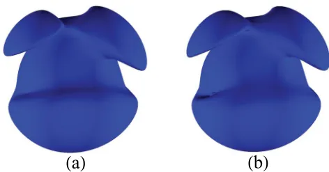
drops seven orders of magnitude, and in contrast,χ2of case 3 withRB=20 drops eight orders. Our ability to retrieve the initial condition is shown for case 3 in physical, rather than spectral space, in Fig.11; the recovery of the|B|isosurface is excellent.
0.2 0.4 0.6 0.8 1.0r 0.05
0.10 0.15
S10 cr
0.2 0.4 0.6 0.8 1.0r
0.10 0.08 0.06 0.04 0.02
S11 cr
0.2 0.4 0.6 0.8 1.0r 0.02
0.04 0.06 0.08 0.10
S11 s r
0.2 0.4 0.6 0.8 1.0r 0.01
0.02 0.03 0.04 0.05 0.06 0.07
S20 cr
0.2 0.4 0.6 0.8 1.0r
0.020 0.015 0.010 0.005
S21 cr
0.2 0.4 0.6 0.8 1.0r 0.005
0.010 0.015 0.020 0.025 0.030
S21 s r
0.2 0.4 0.6 0.8 1.0r
0.010 0.008 0.006 0.004 0.002
S22 cr
0.2 0.4 0.6 0.8 1.0r 0.005
0.010 0.015 0.020
S22 sr
0 100 200 300 400 500N 10
10 10 0.001
0.1 χ2
[image:11.608.315.557.534.693.2] [image:11.608.50.295.654.753.2]0.2 0.4 0.6 0.8 1.0r 0.1
0.2 0.3 0.4
T10 cr
0.2 0.4 0.6 0.8 1.0r
0.25 0.20 0.15 0.10 0.05
T11 cr
0.2 0.4 0.6 0.8 1.0r 0.05
0.10 0.15
T11 sr
0.2 0.4 0.6 0.8 1.0r 0.05
0.10 0.15 0.20 0.25
T20 cr
0.2 0.4 0.6 0.8 1.0r
0.07 0.06 0.05 0.04 0.03 0.02 0.01
T21 cr
0.2 0.4 0.6 0.8 1.0r 0.005 0.010 0.015 0.020 0.025 0.030 0.035
T21 sr
0.2 0.4 0.6 0.8 1.0r 0.02
0.04 0.06 0.08 0.10
T22 cr
0.2 0.4 0.6 0.8 1.0r
0.07 0.06 0.05 0.04 0.03 0.02 0.01
T22 sr
[image:12.608.316.556.73.229.2]0 100 200 300 400 500N 10 10 10 0.001 0.1 χ2
FIG. 6. For the Hall-effect problem, case 1: The rebuilt toroidal initial condition (in solid gray) against the true state (in dashed black) and the reduction of the misfit as a function of the iteration numberN for the Hall-effect problem for 500 equally spaced 3D observations in 7000 years withRB=5.
0.2 0.4 0.6 0.8 1.0r 0.05
0.10 0.15
S10 cr
0.2 0.4 0.6 0.8 1.0r
0.10 0.08 0.06 0.04 0.02
S11 cr
0.2 0.4 0.6 0.8 1.0r 0.02
0.04 0.06 0.08 0.10
S11 sr
0.2 0.4 0.6 0.8 1.0r 0.01 0.02 0.03 0.04 0.05 0.06 0.07
S20 cr
0.2 0.4 0.6 0.8 1.0r
0.020 0.015 0.010 0.005
S21 cr
0.2 0.4 0.6 0.8 1.0r 0.005 0.010 0.015 0.020 0.025 0.030
S21 sr
0.2 0.4 0.6 0.8 1.0r
0.010 0.008 0.006 0.004 0.002
S22 cr
0.2 0.4 0.6 0.8 1.0r 0.005
0.010 0.015 0.020
S22 s r
0 100 200 300 400 500N 10
10 0.001
[image:12.608.55.292.74.227.2]0.1 χ2
FIG. 7. For the Hall-effect problem, case 2: The rebuilt poloidal initial condition (in solid gray) against the true state (in dashed black) and the reduction of the misfit as a function of the iteration numberN for the Hall-effect problem for 500 equally spaced 2D observations in 30 000 years withRB=5.
0.2 0.4 0.6 0.8 1.0r 0.1
0.2 0.3 0.4
T10 cr
0.2 0.4 0.6 0.8 1.0r
0.25 0.20 0.15 0.10 0.05
T11 cr
0.2 0.4 0.6 0.8 1.0r 0.05
0.10 0.15
T11 sr
0.2 0.4 0.6 0.8 1.0r 0.05
0.10 0.15 0.20 0.25
T20 cr
0.2 0.4 0.6 0.8 1.0r
0.06 0.04 0.02
T21 cr
0.2 0.4 0.6 0.8 1.0r 0.01
0.02 0.03
T21 sr
0.2 0.4 0.6 0.8 1.0r 0.02
0.04 0.06 0.08 0.10
T22 cr
0.2 0.4 0.6 0.8 1.0r
0.07 0.06 0.05 0.04 0.03 0.02 0.01
T22 sr
0 100 200 300 400 500N 10
10 0.001
0.1
χ2
FIG. 8. For the Hall-effect problem, case 2: The rebuilt toroidal initial condition (in solid gray) against the true state (in dashed black) and the reduction of the misfit as a function of the iteration numberN for the Hall-effect problem for 500 equally spaced 2D observations in 30 000 years withRB=5.
0.2 0.4 0.6 0.8 1.0r 0.05
0.10 0.15
S10 cr
0.2 0.4 0.6 0.8 1.0r
0.10 0.08 0.06 0.04 0.02
S11 cr
0.2 0.4 0.6 0.8 1.0r 0.02
0.04 0.06 0.08 0.10
S11 sr
0.2 0.4 0.6 0.8 1.0r 0.01 0.02 0.03 0.04 0.05 0.06 0.07
S20 cr
0.2 0.4 0.6 0.8 1.0r
0.020 0.015 0.010 0.005
S21 cr
0.2 0.4 0.6 0.8 1.0r 0.005 0.010 0.015 0.020 0.025 0.030
S21 sr
0.2 0.4 0.6 0.8 1.0r
0.010 0.008 0.006 0.004 0.002
S22 cr
0.2 0.4 0.6 0.8 1.0r 0.005
0.010 0.015 0.020
S22 sr
[image:12.608.52.292.305.458.2]0 100 200 300 400 500N 10 10 10 0.01 1 χ2
FIG. 9. For the Hall-effect problem, case 3: The rebuilt poloidal initial condition (in solid gray) against the true state (in dashed black) and the reduction of the misfit as a function of the iteration numberN for the Hall-effect problem for 500 equally spaced 2D observations in 7000 years withRB=20.
0.2 0.4 0.6 0.8 1.0r 0.1
0.2 0.3 0.4
T10 cr
0.2 0.4 0.6 0.8 1.0r
0.25 0.20 0.15 0.10 0.05
T11 cr
0.2 0.4 0.6 0.8 1.0r 0.05
0.10 0.15
T11 s r
0.2 0.4 0.6 0.8 1.0r 0.05
0.10 0.15 0.20 0.25
T20 cr
0.2 0.4 0.6 0.8 1.0r
0.07 0.06 0.05 0.04 0.03 0.02 0.01
T21 cr
0.2 0.4 0.6 0.8 1.0r 0.005 0.010 0.015 0.020 0.025 0.030 0.035
T21 s r
0.2 0.4 0.6 0.8 1.0r 0.02
0.04 0.06 0.08 0.10
T22 cr
0.2 0.4 0.6 0.8 1.0r
0.07 0.06 0.05 0.04 0.03 0.02 0.01
T22 s r
0 100 200 300 400 500N 10 10 10 0.01 1 χ2
FIG. 10. For the Hall-effect problem, case 3: The rebuilt toroidal initial condition (in solid gray) against the true state (in dashed black) and the reduction of the misfit as a function of the iteration numberN for the Hall-effect problem for 500 equally spaced 2D observations in 7000 years withRB=20.