This is a repository copy of
Intermediate inputs and the export gravity equation
.
White Rose Research Online URL for this paper:
http://eprints.whiterose.ac.uk/77015/
Monograph:
Navas, A., Serti, F. and Tomasi, C. (2013) Intermediate inputs and the export gravity
equation. Research Report. Department of Economics, University of Sheffield ISSN
1749-8368
2013014
[email protected] https://eprints.whiterose.ac.uk/
Reuse
Unless indicated otherwise, fulltext items are protected by copyright with all rights reserved. The copyright exception in section 29 of the Copyright, Designs and Patents Act 1988 allows the making of a single copy solely for the purpose of non-commercial research or private study within the limits of fair dealing. The publisher or other rights-holder may allow further reproduction and re-use of this version - refer to the White Rose Research Online record for this item. Where records identify the publisher as the copyright holder, users can verify any specific terms of use on the publisher’s website.
Takedown
If you consider content in White Rose Research Online to be in breach of UK law, please notify us by
Intermediate Inputs and the Export Gravity Equation
Antonio Navas
Francesco Serti
Chiara Tomasi
ISSN 1749-8368
SERP no. 2013014
Intermediate inputs and the export gravity equation
∗Antonio Navasa, Francesco Sertib, and Chiara Tomasic
aDepartment of Economics, The University of Sheffield
bDepartamento de Fundamentos del Analisis Economico, Universidad de Alicante cUniversity of Trento, Italy, and LEM, Scuola Superiore Sant’Anna, Italy
October 16, 2013
Abstract
This paper introduces imports in intermediate inputs into a standard heterogeneous firms model of trade with asymmetric countries. The model highlights how imports from a specific country affects a firm’s decision to export to that country (the extensive margin), as well as its export value (the intensive margin). The model shows that the effect of both distance and market size on the export margins is magnified when imports in intermediates are accounted for. Indeed, to the extent that exporting firms also use foreign intermediate inputs, the impact of traditional gravity forces on exports also depends on import activities. Exploiting data on product-destination level transactions of a large panel of Italian firms, the paper provides empir-ical evidence in support of the predictions of the model. Controlling for firm-level time-varying unobserved heterogeneity and for the potential endogeneity of firm-level import decisions, the empirical analyses confirm that the estimated elasticities of exports to distance and market size depend on firms’ importing activities.
JEL codes: F12, F14
Keywords: Imports, Exports, Firm heterogeneity, Gravity equation.
1
Introduction
A growing empirical and theoretical literature has emphasised the importance of firm heterogeneity in trade. The burgeoning micro-econometric studies on international trade have mostly focused on exports, while imports have been relatively neglected. Even less attention has been given to firms engaged in a combination of both imports and exports. This is quite surprising given the increasing international fragmentation of production, implying that more and more firms are active in both imports and exports of intermediates and final goods (Hummels et al.; 2001). Only very recently new research on firm heterogeneity and trade has started combining information on both the import and export sides. The available studies show that the majority of exporters are also importers and vice versa. These firms, which have been labeled as two-way traders, account for the bulk of a country’s total trade (Bernard et al.; 2007; Mayer and Ottaviano; 2008; Muuls and Pisu; 2009). Furthermore, a few studies have addressed the key role that imports have in enhancing manufacturing exports. The results suggest that imports positively affect a firm’s probability to become an exporter, as well as its export value and scope (Kasahara and Lapham; 2013; Bas and Strauss-Kahn; 2010).
We contribute to this new strand of literature by investigating previously unexplored effects of the connection between an individual firm’s import and export outcomes. Precisely, the paper studies the consequent influence that the complementarity between the two trade activities has on the export gravity equation, at the firm level. The basic form of the gravity equation relates exports to the economic size and the geographical distance of the destination market, with the latter used as a proxy for transportation costs. The recent trade models with heterogeneous firms show that the gravity forces affect exports via both the extensive and intensive margins of trade (Melitz; 2003; Chaney; 2008; Helpman et al.; 2008). Accordingly, higher market size or lower distance increase the probability that a firm exports to a particular destination as well as its export value to that market.1 However, whether a firm is importing or not may be crucial to evaluate the overall impact that market size and distance have on its export patterns.
This paper derives and estimates the export gravity equation for both the extensive and intensive margins of trade among asymmetric countries in the presence of imports in intermediate inputs. Our theoretical framework follows Chaney (2008) which derives the gravity equation for final good exports in a model of trade with firm heterogeneity. As in Chaney (2008) countries are asymmetric and differ in terms of size, labour costs, trade and institutional barriers. In addition, our model introduces an intermediate input sector. To produce, firms in the final good sector use labor and a continuum of intermediate inputs from different locations. The technology is similar to early endogenous growth models (Romer; 1990; Rivera-Batiz and Romer; 1991), which use a Cobb Douglas specification in which there is love of variety in intermediate inputs.
Two main implications emerge from our setting. First, the exports of final goods are more reactive to distance in the presence of imports in intermediate inputs. A decline in transportation costs (i.e. in distance) has, in fact, a comparatively larger impact on a firm’s probability of exporting and on its export value. This is because, in addition to the standard direct effect found in the gravity model, a reduction in transportation costs also decreases the cost of imported inputs, thus allowing firms to offer their exports at lower prices and to increase their revenues in the exporting markets. Second, following a similar reasoning the presence of intermediate imports amplifies the effect of the foreign market size. The intuition is that the bigger the foreign country, the larger the mass
1As suggested in Crozet and Koenig (2010), the definition employed in this paper for the intensive margin of
of imported inputs and the lower the marginal cost of production. Importing from bigger markets determines larger efficiency gains and thereby increases a firm’s export performance. Thus, foreign market size exerts a positive effect on exports also indirectly through an efficiency increase induced by imports of intermediate inputs.
Our model is also able to reproduce some stylized facts which have emerged from the recent empirical literature. New research show that there is a positive correlation between imports and a firm’s productivity. More generally, importers display similar characteristics to those observed for exporters (Bernard et al.; 2007). The evidence points to the presence of fixed costs not only of exporting, but also of importing and to a process of self-selection in both export and import markets (Kasahara and Lapham; 2013; Castellani et al.; 2010). Also, many theoretical and empirical studies have recognised that imports of intermediate and capital goods can raise productivity via several channels: learning, variety and quality effects.2 In line with these findings our theoretical framework predicts that the relatively more productive firms self select into importing and that only a subset of the most productive firms undertake both trade activities. Moreover, the model shows that importing increases a firm’s productivity, through a better reallocation of resources across new intermediate inputs.
We test the main predictions of our model by exploiting an original Italian database obtained by merging a firm-level dataset, including standard balance sheet information, with a transaction-level dataset, recording custom information on exports and imports for each product and destination. The key advantage of our data is that we know, for each firm in the panel, whether a firm exports or imports, how much it trades, and where it exports to or imports from. Moreover, by exploiting the product information we can distinguish whether a firm’s imports are intermediate inputs. Firm-level trade data are complemented by country characteristics including proxies for market size, distance, variable and fixed trade costs.
All the empirical results support the theoretical predictions of the model showing that, both on the extensive and the intensive margins, the estimated elasticities of exports to distance and GDP depend on firms’ importing activities.
Within the vast empirical literature on firm heterogeneity in international trade, this article directly relates to the emerging literature on the interdependence between importing and exporting activities. A leading recent theory is provided by Kasahara and Lapham (2013) who develop a symmetric country model on the import-productivity-export nexus. In their theoretical framework the use of foreign intermediates increases a firm’s productivity but, because of the existence of fixed costs of importing, only the most productive firms are able to source from abroad. In turn, productivity gains from importing allows some importers to start exporting. In a similar framework, Nocco (2012) studies the consequences for average productivity and welfare of trade liberalisation in a model of trade with vertical linkages,obtaining that the results clearly depend on the share of intermediate inputs in the total production of the final good. Unlike these papers, we extend the Melitz (2003) model to incorporate trade in intermediates in an asymmetric country environment. The latter allows us to derive the gravity equation and to include cross country determinants of export and import activities across firms, which is the focus of the paper. The causal link from intermediate inputs to final good exports is also tested in Bas and Strauss-Kahn (2010). Using French firm level data the study shows that a larger variety of imported inputs, increases firms’ productivity and firms with high productivity levels export more varieties. The importance of imported intermediates for exports is also implied by Feng et al. (2012), who find that Chinese
2For a theoretical background of the productivity gains induced by intermediate inputs see Markusen (1989);
firms that increased the expenditure and the varieties of imported inputs enlarged the value and the scope of their exports.
Our paper is also strongly connected to the literature on the gravity equation. Applied for the first time by Tinbergen (1962), the equation shows that trade between two countries is proportional to their respective sizes, measured by their GDP, and inversely proportional to the geographic distance between them. The heterogeneous-firm model brings to the gravity model a need to consider the effects of trade barriers both on the value of exports by current exporters and on the entry of exporters. In his model Chaney (2008) extends the work of Melitz (2003) to show that there is both an intensive and an extensive margin of adjustment of trade flows to trade barriers. In a similar manner, Helpman et al. (2008) derive a gravity equation and develop an estimation procedure to obtain the effects of trade barriers and policies on the two margins. Empirical analyses that use firm-country level data confirm several of the theoretical predictions. Eaton et al. (2011, 2004) for France and Bernard et al. (2007) for the US find that the number of exporting firms is sharply decreasing in the distance to the destination country and increasing in importer income. Crozet and Koenig (2010) use French data to estimate the structural parameters of Chaney’s model and show by how much the foreign sales of a given set of firms and by how much the number of firms respond to changes in trade costs. By estimating an export firm-level gravity equation, other empirical studies offer evidence that both firm-level productivity and market-specific trade costs affect individual export decision and export sales to a particular destination (Lawless and Whelan; 2008; Smeets et al.; 2010).
None of the cited studies, however, consider the role played by imports in the export firm level gravity equation. Indeed, while it has been already established that market size and distance are crucial in shaping exports patterns, it is an open question whether and how importing plays a role in the gravity mechanisms. This paper provides a micro-foundation for the export gravity equation with imports in intermediate inputs.
The remained of the paper is organized as follows. Section 2 presents a trade model with heterogeneous firms, featuring imports in intermediate inputs to derive the export gravity equation, both at firm and industry level. Section 3 introduces the strategy in the empirical analysis and describes the data for the empirical study. Section 4 presents the estimation results and Section 5 concludes.
2
The model
The aim of this section is to motivate our empirical analysis by introducing a partial equilibrium model to study the effects of imports in intermediate inputs in the export gravity equation at the firm level. The model is based on Chaney (2008), which extends Melitz (2003) to incorporate trade between asymmetric countries. To the latter framework we add an intermediate input sector and we allow for trade in both intermediate inputs and final goods.
2.1 Preferences
ConsiderN potential asymmetric countries, indexed byn, each of them populated by a continuum of individuals of measure Ln who derive utility from the consumption of the H + 1 final goods
existing in the economy according to the following functional form
U =
H Y
h=0
(Qhn)µh,
H X
h=0
where Qhn represents consumption of final good h in the generic country n. Sector 0 produces an
homogeneous good. Each of the rest of the H different sectors produces a continuum of varieties
ω in the set Ωh. Preferences across different varieties of the same final good are described by the
CES utility function
Qhn=
Z
ωǫΩh
(qhn(ω))
σh−1 σh dω
σh σh−1
, σh>1
where the parameterσh controls for the elasticity of substitution across varieties within the sector
h.Solving for the consumer’s maximization problem we obtain the demand function for each variety within each sector
qhn(ω) =
µhRn
Phn
p
hn(ω)
Phn
−σh
where Rn, Phn represents respectively income and the standard CES aggregate price index for
countryn.3
2.2 Production
Production of the homogeneous good uses labor as an input. The technology is linear, described by the following functional form
q0n=εnl0n.
Assuming that this good is produced under perfect competition and taking this good as the numeraire, profit maximization will imply thatwn=εn.Each firm produces a unique differentiated
variety. To produce, each firmf in the final good sectorh needs to incur in per period fixed costs of operationfh (in units of the numeraire). In contrast to Chaney (2008) we assume that firms use
intermediate inputs and labor to produce. More precisely, each firm produces using the following Cobb-Douglas technology
qhnf =ϕfhlhnf 1−αhmfhnαh (1)
wherelhf denotes labor dedicated to production,mfhn=
Z
νǫΛ
mfhn(ν)
φh−1 φh dν
φh φh−1
is the
inter-mediate composite input used in sector h where mfhn(ν) is firm f’s demand of the intermediate input variety ν produced in country n, and ϕfh denotes firms’ productivity. The parameterφh >1
controls for the degree of substitutability across intermediate inputs within a sector. The param-eter αh measures the importance of intermediate inputs in the production of each final good. We
assume that the elasticity of substitution across intermediate inputs is a technological parameter and therefore it is common across all countries though it may differ across sectors. Following Romer (1990) and Rivera-Batiz and Romer (1991), we have assumed that there is love of variety in the set of intermediates and each firm within each country offers a unique variety either in the final
3P hn=
Z
ωǫΩh
(phn(ω))1−σhdω
1 1−σh
good sector or in the intermediate input sector. The former will be crucial to obtain the result according to which that importing intermediate inputs has a positive impact on a firm’s total factor productivity.
As it is common to this literature, we assume that the firms’ productivity is stochastic. More precisely, we assume that ϕfh follows a Pareto distribution with cumulative density function given by
Pr(ϕfh < ϕ) = 1−ϕ−γh (2)
with γh controlling for the productivity dispersion within sectors. Following the broad literature
on trade and firm heterogeneity we assume γh > σh−1 andγh >2. At the moment of entry each
firm takes a draw from this common productivity distribution. This determines the productivity of the firm that for simplicity we assume that is constant over time.
In the intermediate input sector, each firm within each country is producing a unique variety. To produce it, the firm uses a simple linear technology where labor is the unique production factor
m(ν) =lm. (3)
We assume, as in Chaney (2008), that the mass of entrants is proportional to the income of the economy (i.e. wnLn). In this setup, however, we need to make an extra assumption about
how the prospective entrants are distributed among theH+ 1 differentiated sectors. We posit that an exogenous percentage of those entrantsβhn enters in the final good sector h and a proportion
βmn = (1−
H X
h=1
βhn) enters in the intermediate sector. Therefore, our modeling strategy allows
two different stages of production characterized by two different sets of tradable goods, final goods and intermediate inputs. However, for the sake of simplicity, the country level determinants of the allocation of resources across the two production stages are left unmodeled.
To complete the definition of the model we assume that all existing firms in the world belong to a mutual fund and each individual in each country ownswn shares of this mutual fund. In this
model entry is exogenous, and since firms earn positive profits in each of the final good sectors and the intermediate input sector, we should assume a way to redistribute positive profits across consumers. Since income distribution does not affect the aggregate variables in this model all our results will be robust to any alternative way of redistributing profits across individuals.
2.3 Trade
In our world there exists trade in both final goods and intermediate inputs. Moreover, both activities bear fixed and variable costs. More precisely, a firm in countryk,which wants to export to country
j, must pay a fixed cost fhxkj (in units of the numeraire) and variable costs of the iceberg type
τhxkj. We follow Anderson and van Wincoop (2004) in assuming that τhxkj, the variable export
costs in sectorh, are a loglinear function ofDkj, the distance between countries, and ∆hxkj, other
variable costs which are not related to distance (i.e. export tariffs). Export variable trade barriers are given by the following functional form
τhxkj = ∆hxkj(Dkj)δh, (4)
where ∆hxkj>1 ifk6=j.4
4If one unit of the good is shipped from countrykto countryj, only a fraction 1/τ
kj reaches countryj. τkj>1
for anyk 6=j . We assume as well thatτkk = 1 and the following triangular inequality: τkn ≤τkj×τjn for any
Firms have also the option to import intermediates from abroad by incurring a fixed cost offhik
in units of the numeraire. Exporting intermediates is also subject to variable costs of the iceberg typeτhmjk. We assume that variable costs related to distance are the same for final good exporters
and intermediate exporters, but we allow for differences in the other variable costs
τhmjk = ∆hmjk(Dkj)δh. (5)
The inclusion of fixed costs in both activities implies that not all firms are going to find it profitable either to export final goods or to import intermediates. Consistent with the above stylized facts, we are going to show that only those firms that overcome a threshold productivity level will find it profitable to engage in foreign activities and only a subset of these ones, which will be the most productive ones, will find profitable to engage in both activities.
2.4 The firm-level export gravity equation
Since the model is deterministic, depending on the parameters’ configuration we can have different types of equilibria. In this paper, we focus on equilibria where the firms engaged in international trade are either both exporters of final goods and importers of intermediate products or just only importers.5
Each intermediate input producer is a monopolist of its own variety. This implies that the price the intermediate producer charges will be given byphmk =ρhmτhmjkwj whereτhmjj= 1 and
ρhm= φφh−h1 is the firm’s mark-up.6 The intermediate input producer charges a higher price to the
foreign market because it is more costly to serve the foreign market.
In the final good sectors, the firm profit maximization problem can be described in two steps. In the first step, the cost minimization problem, firms choose the optimal combination of inputs for a given production quantity, while in the second step they choose the price (and therefore indirectly the quantity sold) they will charge to consumers for their differentiated product. Solving the first step we obtain that the variable cost of production associated to a firm in country k is given by the following expression7
chk
ϕf= (wk)
1−αh(P
hmk)αh
Γh
qhkf
ϕf =
(ρhm)αhwk
Γh(χhk)d
˜
Lk
αh
φh−1
qhkf
ϕf (6)
which is a linear function of the quantity, χhk =
N X
j=1
w
j
wk
τhmjk
1−φh L˜j
˜
Lk
αh φh−1
, d is a dummy
variable taking the value 1 if the firm imports intermediates, Γh is a technological constant, and
˜
Lk = βmkwkLk.8 Notice that χhk > 1,and consequently, importers, ceteris paribus, enjoy lower
marginal costs of production.
In the second step of the profit maximization problem, as usual in the Dixit Stiglitz monopolistic competition framework, the price set by firms is a constant mark-up over marginal costs. Therefore,
5The empirical analysis on Italian data reveals that the export productivity premia is higher than the import
productivity premia suggesting that the productivity threshold required for exporting is greater than that one for importing (results are available upon request). This is consistent with the equilibrium we focus in our theoretical model.
6Note that the mark-upρ
hm is the same for foreign intermediate producer and domestic intermediate producers. 7Details about how to derive this analytical result can be found in the appendix.
8Γ
the price on marketj of a final good produced in countrykby a firm with productivity ϕf is
phxkj(ϕf) =
σh
σh−1
(ρhm)αh
Γh(χhk)d
˜
Lk
αh
φh−1
τhxkjwk
ϕf . (7)
Substituting (7) in the demand function we obtain the quantity sold in country j by a final good producer of countryk,which is
qhxkj(ϕf) =
µhRj
(Phj)1−σh
τhxkjρh(ρhm)αhwk
Γhχhk
˜
Lk
φhαh−1
ϕf
−σh
, (8)
whereρh = σσh
h−1 is the mark-up of final goods producers belonging to sectorh; notice that we have
denoted with subscriptj the demand variables referring to country j.
The variable profits from selling to country j for a firm producing in sector h, in countryk is given by
rhxkj(ϕf) = (τhxkj)1−σh
µhRj
σh(Phj)1−σh
ρh(ρhm)αwk
Γhχhk
˜
Lk
αh
φh−1
ϕf
1−σh
. (9)
A firm of country k will export to country j when rhxkj(ϕf) ≥fhxkj.Hence, the productivity
of the marginal firm which is indifferent between exporting and not exporting to countryj is given by the following cutoff
ϕ∗hxkj =τhxkj
σh
µh
1
σh−1 1
Rj
1
σh−1
ρh(wk) (Phj)−1(fhxkj)
1 σh−1
(ρhm)α
˜
Lk
α
1−φh
χhkΓh
| {z }
Interm.Inputs
. (10)
This expression is identical to the one derived in a model without intermediate inputs except for the last term. This equation determines the probability of exporting to a specific destinationj.
In a further section we discuss the main variables influencing this probability.
A firm ink is willing to import intermediates from the rest of the world if the gains in revenue from importing intermediates overcome the fixed cost of importing fhik. We focus on equilibria
where the marginal importing firm is not an exporter. To obtain the productivity cutoff associated with importing we first consider the revenue that an importing firm has in the domestic market, which is given by 9
rhik(ϕf) =
µhRk
σh(Phk)1−σh
ψhwk
χhk
˜
Lk
φhαh−1
ϕf
1−σh
(11)
where for simplicity we denote ψh = ρh(ρhm)
αh
Γh . A firm in k which is not an importer obtains the
following domestic revenue
rhk
ϕf= µhRk
σh(Phk)1−σh
ψhwk
˜
Lk
αh
φh−1
ϕf
1−σh
. (12)
9Note that r
hik is the revenue of a firm importing intermediate inputs and producing final goods only for the
Note that rhik(ϕf) = (χhk)σh−1rhk ϕf
. A firm in k will be importing intermediates from abroad ifrhik(ϕf)−rhk(ϕf)≥fhik.The marginal firm, the one that is indifferent between importing
and not importing, satisfies the following condition
(χhk)σh−1−1
µhRk
σh(Phk)1−σh
ψh(wk)
˜
Lk
αh
φh−1
1−σh
(ϕ∗hik)σh−1=f
hik.
The threshold productivity level associated with importing intermediates from abroad (for a firm that is only importing) is given by
ϕ∗hik = 1
((χhk)σh−1−1) 1 σh−1
σh
µh
1
σh−1 1
Rk
1
σh−1
ψhwk(Phk)−1
·(fhik)
1 σh−1
˜
Lk
1−αh
φh .
(13)
In this case the lower are the variable trade costs (the larger χhk) the lower is the import
threshold productivity level. Indeed, as variable trade costs are reduced, foreign intermediate inputs become cheaper, and, as a consequence, more firms are able to bear the fixed costs of importing. Clearly, larger fixed costs of importing goods are associated with a more stringent productivity threshold, or less firms importing. Finally, the larger is the home market, the larger is the mass of importing firms. This is due to two different mechanisms. On the one hand, a larger home market,
Rk,implies a larger demand of final goods and, as a consequence, a larger demand of intermediate
inputs. On the other hand, firms in larger markets have access to a larger set of intermediate inputs and, therefore, have a lower marginal cost. As the gains from importing intermediates from abroad are inversely proportional to the marginal cost of production, firms’ profits from importing intermediates are larger in larger markets.
Finally, the survival productivity threshold is described by the following equation
ϕ∗hk=
σh
µh
1
σh−1 1
Rk
1
σh−1
(ψhwk) (Phk)−1(fh)
1 σh−1
˜
Lk
1−αh
φh . (14)
Given the basic ingredients of the model - preferences, technologies and the optimal strategies of firms - we need now to derive the equilibrium aggregate price index for each economy so to obtain the gravity equation for exports of final goods. Initially we have considered the aggregate price indexes Phj as given, disregarding the fact that they adjust depending on country characteristics.
The economy j aggregate price index Phj can be easily obtained considering that
P1−σh
hj =βhjwjLj
∞
Z
ϕ∗
hj
(phj(ϕ))1−σhg(ϕ)dϕ
| {z }
Domestic firms
+
N X
n6=j
βhnwnLn
∞
Z
ϕ∗
hxnj
(phxnj(ϕ))1−σhg(ϕ)dϕ
| {z }
Foreign exporters
.
∞
Z
ϕ∗
hj
(phj(ϕ))1−σhg(ϕ)dϕ= ϕ∗
hij
Z
ϕ∗
hj
(phj(ϕ))1−σhg(ϕ)dϕ+
∞
Z
ϕ∗
hij
(phij(ϕ))1−σhg(ϕ)dϕ
where phj(ϕ) denotes the price that domestic firms which do not import charge in the domestic
market and phij(ϕ) is the price that domestic firms that import charge in the domestic market.
Notice thatphj(ϕ) =χhj phij(ϕ) and therefore non importing firms charge higher prices.
Substi-tuting the expression for optimal pricing for each firm in each market and rearranging terms we obtain
Phj =λ2h(Yj)
1 γh−
1 σh−1 θ
hj (15)
where
(θhj)−γh= N X n=1 Yn
Y (wnτhxnj)
−γh(f
hxnj)
σh−γh−1 σh
(1−ξ)
| {z }
Chaney′s
βhn
˜
Ln
αhγh
φh−1
ψ−γh
h χ
γh
hn (1−ξ)
(Φh)ξ
λγh
2h =
γh−(σh−1)
γh
σh
µh
σh1−−γh−1
σh 1 +π Y
and
Φh = (fh)
σh−γh−1
σh−1
+(χhn)σh−1−1
γh
σh−1
(fhin)
σh−γh−1
σh−1
.
The variable ξ is a dummy taking the value of 1 ifn=jand 0 otherwise.10 θhj is an aggregate
index ofj’s remoteness from the rest of the world. With respect to Chaney (2008), this “multilateral resistence variable” also takes into account that, in this case, the price of final goods depends also on the cost of intermediate inputs. The larger the access of country j to intermediate inputs sources, the lower will be the probability of exporting to countryj.
In what follows we assume that our country is a small open economy. This implies that any change in the domestic market does not have any relevant impact on the measure θhj′ , the mul-tilateral resistance term. This simplifies significantly the calculations. With the definition of the price index in hand, we are able to derive the general equilibrium value of the export productivity cutoffs and of firm-level exports.
Plugging (15) in (10) and using the fact that Rj =Yj, we obtain the equilibrium value of the
productivity threshold for exports. Then the probability that a firm in countrykexports to country
j is given by
Pr(ϕ≥ϕ∗hxkj) = ϕ∗hxkj−γh
= λ′4h−γh
Y
j
Y
w
kτhxkj
θhj′
!−γh
(fhxkj)
−γh
σh−1
| {z }
Chaney′s
( ˜χhk)γh | {z } new elements
(16)
where λ′4h is a constant11 and ˜χhk =χhk
βmkYk
Y
αh
φh−1 12
. This is the gravity equation at the firm level for the extensive margin of trade. It relates the standard elements found in a gravity equation to the probability that a firm in k exports to country j (and therefore the mass of firms in k
exporting to country j).Foreign market size contributes positively to the mass of firms exporting to countryj. Barriers to exports (both fixed and variable costs) reduce the probability of exporting. The multilateral resistance term affects positively the mass of firms exporting, that is, the larger are trade barriers of a trade partner with the rest of the world, the larger is the mass of country
kfirms exporting to such destination. The novelties with respect to a model without intermediate inputs are related to the last element of equation (16). The inverse of this element represents the cost of the basket of intermediate inputs that the firm is using. The smaller the cost is the larger is the probability that a firm exports to countryj.
To see what are the main determinants of the value of the exports to countryj for a firm with productivity ϕf ≥ϕ∗xkj, it is useful to express firms’ revenue from the export market as
rhxkj(ϕf) =
ϕf
ϕ∗
hxkj !σh−1
rhxkj(ϕ∗hxkj)
= λ′3h
Y
j
Y
σh−1
γh θhj′
wkτhxkj
!σh−1
| {z }
Chaney′s
( ˜χhk)σh−1
| {z }
new element
ϕfσh−1
(17)
where λ′3h is a constant.13 This is the gravity equation for the intensive margin of trade. The individual export value increases with destination market size and countryj′sremoteness from the rest of the world and decreases with variable trade costs.
The next section describes in detail what are the main predictions of this model. Some of the results predicted by the model are already familiar in the empirical literature, while some of them are entirely new. The empirical part focuses on testing these new results.
2.5 The predictions of the model
This section presents the main predictions of the model. The very first set of results focuses on the impact that importing intermediates has on a firms’ TFP. These results have been recently the focus of the attention of a broad set of empirical papers.
11λ′
4h=
γh
γh−(σh−1)
γh1
σh
µh
γh1
(1 +π)−1γh 1+π Y
φhαh −1.
Notice that this constant is similar to the corresponding one derived in Chaney’s paper. There are however two main differences: First the last term that is purely due to the existence of intermediate inputs (since the market size has an extra effect), to transform this measure of market size in country’s k GDP we need to multiply by that constant. The second one will correspond to the aggregate profits, whose expression will be different in this paper. Apart from the profits in the final good sector that will change we need to take into account as well the profits in the intermediate good sector.
12More precisely χ˜
hk = χhk
βhkYk
Y αh φh−1 = "N X j=1 w j
wkτhmjk
1−φhβ
mj
βmk
Y
j
Yk
βmkYk
Y
#φhαh−1 = "N X j=1 w j
wkτhmkj
1−φh
βhj Yj
Y
#φhαh−1
13Following Chaney (2008) notationλ′
3h=σ(λ′4h) 1−σ
Proposition 1 Importing intermediate inputs has a positive effect on a firm’s productivity.(TFP)
Proof. See appendix
This result is a consequence of the love of variety assumption. The technology, similar to Romer (1990), presents decreasing returns to scale in the use of each intermediate input and increasing returns to scale in the mass of varieties used. A firm importing intermediates from abroad is able to escape from the decreasing returns to scale associated with each of the intermediate inputs currently used by the firm by splitting its intermediate input requirements across more varieties. The ability of the firm to do so clearly depends on the mass of imported intermediate inputs available, as well as on the price of each intermediate input. Since both variables vary across destinations, the model also predicts heterogeneous gains across source countries.
The statement of Proposition 1 is consistent with the empirical findings of Kasahara and Ro-drigue (2008); Halpern et al. (2011); Bas and Strauss-Kahn (2010), which observe a positive link between importing intermediates and productivity.
Corollary 1.1 The productivity benefits from importing intermediate inputs decrease with variable trade costs, increase with the foreign country size and, under certain conditions, with the income per capita (i.e. the wage) of the source country.
Proof. See appendix
The larger the size of the source country, the larger the mass of intermediate inputs available. As a consequence a firm can split its intermediate input requirements across more varieties, having a stronger impact on productivity. The variable trade costs affect negatively the cost of interme-diate inputs from abroad. The latter limits the ability of a firm to spread its intermeinterme-diate input requirements across varieties coming from that destination. Concerning the income per capita of the source country (i.e. the wage14), there are two opposite effects. On the one hand, intermediates coming from rich countries are more expensive. This limits the scope of a firm to take advantage from the access to a larger range of varieties in a similar way as transportation costs do, with a negative impact on a firm’s TFP. On the other hand, richer countries produce more varieties. It can be shown that the second effect dominates the first one provided thatφh <2,or in other terms,
the intermediate inputs are not substitutable enough.
The second set of results focuses on the role played by intermediates imports in the gravity equation, both in terms of the extensive and intensive margins of exports. We will start by consid-ering the implications for the extensive margin of trade. The introduction of imported intermediate inputs in the basic Melitz/Chaney model has two main consequences with respect to the export productivity cutoff expressed by equation (16).
Proposition 2 The effect of distance on the probability of exporting to a specific country is magni-fied by the presence of trade in intermediate inputs. The elasticity with respect to distance is given by
dln(Pr(ϕ≥ϕ∗hxkj))
dln (Dkj)
=−δhγh(1 +αhshmjk).
Proof. See appendix
14We are aware that the income per capita of the economy is given byy j=
Yj
Lj =wj(1 +π) which is not exactly
The inclusion of trade in intermediates in the analysis changes the effects of distance on the probability that a firm in country k exports to country j. To the extent that export and import variable costs have common determinants15, a decrease in transportation costs has a comparatively larger impact on the mass of exporting firms. This is the consequence of the fact that a reduction in distance affects both the price of exports to countryj and the cost of intermediate inputs coming from country j.
The first effect is standard in the literature. A reduction in the costs of serving countryj allows firms to charge lower prices, increasing the value of sales to that country. The expected increase in foreign sales makes exporting more attractive to firms. The latter increases the probability of selling to that country. The second effect is inherent to this framework. A reduction in transportation costs between kand j decreases the cost of importing intermediates from market j. This allows a firm to charge lower prices in countryj too, increasing its export sales. This latter effect is shaped by two parameters: the share of imported intermediate inputs from country j - shmkj - and the
importance of intermediate inputs in the production of the final good -αh.
Proposition 3 The elasticity of the probability of exporting to a specific destination with respect to market size (domestic and foreign) is given by
dln(Pr(ϕ≥ϕ∗hxkj))
dln (Yl)
=ξ+ αhγh
φh−1
shmlk l=k, j.
Proof. See appendix
In this case it is convenient to discuss separately the effect of both the foreign and the domestic market size. An increase in foreign market size has a positive effect on the probability of exporting due to both a direct and an indirect effect. Foreign market size enters directly in equation (16) throughYj. The larger the income level of countryj, the larger the expenditure on final goods and
the market potential of domestic exporters. This reduces the productivity level necessary to cover the fixed costs of exporting to that destination. The positive effect of the country size is magnified by the fact that the foreign market is also a source of intermediate inputs. The larger is the foreign market, the larger is the mass of imported intermediate inputs and the lower is the marginal cost of production. Consequently, firms importing from a large market will be able to charge lower prices, increasing the probability of becoming an exporter to a particular destination.
Novel to this framework, domestic market size also affects the probability of exporting. More populated and more productive economies provide a greater number of varieties of intermediate inputs. Since the marginal costs of production decrease with the amount of intermediate inputs used by the firm, marginal costs of production decrease with the size of the domestic market. The latter gives a competitive advantage to domestic firms in foreign markets.16
Similar implications are derived when we consider the intensive margin of exports. Also in this case, intermediate imported inputs magnify the effects of the traditional gravity forces on the value of exports.
Proposition 4 The effect of distance on a firm’s exports to a specific destination is amplified. The elasticity of a firm’s exports to distance is given by
15Indeed, the model assumes that costs are related to distance in the same way.
16Unfortunately, we are not able to test this prediction since we have information only for one domestic market,
dlnrhxkj(ϕf)
dln (Dkj)
=−δh(σh−1) (1 +αhshmjk).
Proof. See appendix
Proposition 5 The effect of market size on a firm’s exports to a specific destination is amplified. The elasticity of a firm’s exports to market size is given by
dlnrhxkl(ϕf)
dln (Yl)
=
σh−1
γh
ξ+αh(σh−1)
φh−1
shmlk, l=k, j
where the home country size plays also an important role.17 Proof. See appendix
The mechanisms behind the amplification effect in the intensive margin are the same as in the extensive margin. A decrease in transportation costs reduces the cost of importing intermediates. This allows exporting firms to reduce the price charged for their exports and consequently to increase the sales in each market, domestic and foreign. Foreign and domestic market size positively affect the value of exports since these are connected with the mass of intermediate inputs available for the firm. The larger the foreign and the domestic market, the larger is the range of intermediate inputs available for the firm. The latter allows the firm to reduce the price charged for their exports and to increase the value of sales in each market.
In this section we have derived the main predictions of the model. We have shown that including intermediate inputs in the analysis modifies the standard predictions of the effects of distance and market size either on the probability that a firm exports to a particular destination or on the value of exports to that particular destination. The model strongly suggests controlling for measures related to firm intermediate importing activities in order to estimate accurately the effects that traditional gravity forces have on firms’ exporting behaviour. In the next sections, we test these empirical implications using a rich firm-country level Italian dataset.
3
Empirical specification, Data and Facts
We now turn to present the empirical specification adopted to test some of the main predictions of the model. We then describe the firm level dataset used in the analyses and then discuss the country-level variables employed in the regressions. Finally, we discuss some trends and facts regarding firms’ behaviour in international markets.
17In a model without trade in intermediates the elasticities will be equal to: dlnrhxkj(ϕf)
dln(Dkj) =−δh(σh−1)
dlnrhxkl(ϕf)
dln(Yl) =
σh−1
γh
ξ, l=k, j
dln(Pr(ϕ≥ϕ∗
hxkj))
dln(Dkj) =−δhγh
dln(Pr(ϕ≥ϕ∗
hxkj))
3.1 Empirical specification
Having described the theoretical structure of the model and its testable predictions, we now adapt it for the empirical estimations. Equations (16) and (17) describe how the country’s extensive margin of trade (the decision to export or not) and the intensive margin of trade (the export value decision) are related to firm and country characteristics. Equation (16) of our model predicts that the country-by-country entry decision (Entry) depends on firm productivity (ϕ), foreign market size (Y), the multilateral resistance term (θ), variable trade costs (Dand ∆), fixed trade costs (f) and the new element ˜χ. According to equation (17), all these elements, except the fixed trade costs, enter also in the individual export value decision. Indeed, these costs, once paid, do not influence an exporter’s revenues. These two equations together with Propositions 2-5 form the underpinning of our estimations.
We start by specifying a model for the export entry decision. The empirical model for the probability of entry is given by
Entryf jt=αo+b1ϕf t−1+α2Dj +α3Yjt+α4∆jt+α5fj+α6θjt+
+α7Mf jt+α8Mf jt∗Dj +α9Mf jt∗Yjt+di+ǫf jt
(18)
where the dependent variable,Entryf jt, is a dummy variable that takes value one if a firmf starts
exporting to country j at time t and zero otherwise. The focus on the group of starters allows us to disregard the role of the lagged export status on the probability of exporting to country j at time t. Indeed, the international trade literature has strongly emphasized that previous trading status significantly affects the current probability of trading (Roberts and Tybout; 1997; Bernard and Jensen; 2004). Analogously, past participation in a specific market increases the probability that a firm will enter the same market (Lawless and Whelan; 2008).
The empirical specification includes a measure of the firm’s productivity (ϕf t−1) and all the country-level variables included in equation (16) (Yjt,θjt,Dj, ∆jt,fj). We use the lagged value of
ϕto reduce the possibility that the estimated coefficient is not contaminated by possible feedback effects of export decision on firm productivity. We expectα1 to be positive in accordance with our model and, more generally, with the standard literature on the relationship between productivity and exports. The model also predicts that the probability of serving the foreign market j should increase with the size of the country (α3 >0) and the level of remoteness (α6 > 0) and decrease with the level of variable costs (α2<0;α4 <0) and fixed costs (α5<0).
In the empirical framework we also include a proxy for the import share of the firm Mf jt. Note
that in the current version of the model, the intermediate input cost index does not vary at the firm level. This is the consequence of the fact that all firms import from all sources and firm’s intermediate inputs are also proportional to the productivity parameter ϕfσh−1
. However, in reality we observe that firms do not import from all sources and that the share of imports from a particular country varies across firms within the same sector. This implies that we can not control for the intermediate input mechanism just by adding sector fixed effects since this channel will vary also at the firm level. Thus, in the empirical model we include the firm level variable Mf jt
indicating a firm’s share of imported intermediate inputs from country j at time t. We expect a positive impact of imports on the probability of exporting, i.e. α7 > 0. We then interact the two gravity forces with our firm-level measure of imports (Mf jt∗Dj and Mf jt∗Yjt). From our
Our model also includes a set of fixed effect di. By exploiting the three-dimensional nature
(firms, destinations, time) of our dataset, we take time-invariant as well as time-varying firm-level unobserved heterogeneity into account.
The second step of our empirical analysis consists of estimating the determinants of a firm’s exports across countries. The econometric model, which can be thought of as a micro-gravity equation, takes the following form
lnExportsf jt =βo+β1ϕf t−1+β2Dj+β3Yjt+β4∆jt+β5θjt+
+β6Mf jt+β7Mf jt∗Dj+β8Mf jt∗Yjt+di+ǫf jt
(19)
where the dependent variable is the (log) total exports of firm f in country j at time t. As in the previous equation, we include firm productivity, country determinants, and a proxy for the firm’s importing activity. Following equation (17), we exclude the trade fixed costs variable (f). According to Propositions 4 and 5, the effect of distance and foreign market size on a firm’s export value to country j is amplified when imports are taken into account. We thus include in the empirical model the interaction terms Mf jt∗Dj and Mf jt∗Yjt.
3.2 Firm level data
The empirical analysis combines three sources of data collected by the Italian Statistical Office (ISTAT): the Italian Foreign Trade Statistics (COE), the Italian Register of Active Firms (ASIA) and a firm level accounting dataset (Micro 3).18.
The COE dataset is the official source for the trade flows of Italy and it reports all cross-border transactions performed by Italian firms for the period 1998-2003. The database includes the value of the transactions, on a yearly basis, of the firm as disaggregated by countries of destination for exports and markets of origin for imports.19 The total value of a firm-country transaction, recorded in euros, is broken down into five broad categories of goods, Main Industrial Groupings (MIGs), identified by EUROSTAT as energy, intermediate, capital, consumer durables and con-sumer non-durables.20 This is a unique feature of our dataset which allows distinguishing imported intermediate inputs from other types of imports.21
Using the unique identification code of the firm, we are able to link the trade data to ISTAT’s archive of active firms, ASIA. The ASIA register covers the population of Italian firms active in the same time span, irrespective of their trade status. It reports annual figures on number of employees, sector of main activity and information about the geographical location of the firms (municipality of principal activity of legal address). The ASIA-COE dataset obtained by merging the two sources is not a sample but rather includes all active firms.
Data on firm level characteristics come from Micro.3, which is a dataset based on the census of Italian firms conducted yearly by ISTAT containing information on firms with more than 20 employees covering all sectors of the economy for the period 1989-2007.22 Starting in 1998 the
18The database has been made available for work after careful screening to avoid disclosure of individual information.
The data were accessed at the ISTAT facilities in Rome.
19ISTAT collects data on exports based on transactions. The European Union sets a common framework of rules
but leaves some flexibility to member states. A detailed description of requirements for data collection on exports and imports in Italy is provided in Appendix A4.
20EUROSTAT’s end-use categories (Main Industrial Groupings, MIGs), based on the Nace Rev. 2 classification,
are defined by the Commission regulation (EC) n.656/2007 of 14 June 2007.
21Hereafter, when using the word “import” we refer to import of intermediates inputs unless otherwise specified. 22The database has been built as a result of collaboration between ISTAT and a group of LEM researchers from
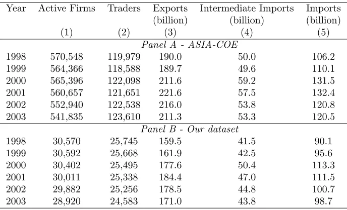
Table 1: COVERAGE OF OUR DATASET
Year Active Firms Traders Exports Intermediate Imports Imports (billion) (billion) (billion)
(1) (2) (3) (4) (5)
Panel A - ASIA-COE
1998 570,548 119,979 190.0 50.0 106.2
1999 564,366 118,588 189.7 49.6 110.1
2000 565,396 122,098 211.6 59.2 131.5
2001 560,657 121,651 221.6 57.5 132.4
2002 552,940 122,538 216.0 53.8 120.8
2003 541,835 123,610 211.3 53.3 120.5
Panel B - Our dataset
1998 30,570 25,745 159.5 41.5 90.1
1999 30,592 25,668 161.9 42.5 95.6
2000 30,402 25,495 177.6 50.4 113.3
2001 30,011 25,338 184.4 47.0 111.5
2002 29,882 25,256 178.5 44.8 100.7
2003 28,920 24,583 171.0 43.8 98.7
Note: Table reports the number of manufacturing firms in ASIACOE and after the merge with Micro3. Panel A -ASIA-COE, Panel B, Our dataset.
census of the whole population of firms only concerns companies with more than 100 employees, while in the range of employment 20-99, ISTAT directly monitors only a “rotating sample” which varies every five years. In order to complete the coverage of firms in that range Micro.3 resorts, from 1998 onward, to data from the financial statement that limited liability firms have to disclose, in accordance to Italian law.23 The database contains information on a number of variables appearing in a firm’s balance sheet. For the purpose of this paper we utilise: number of employees, turnover, value added, capital, labour cost, intermediate inputs costs and capital assets. Capital is proxied by tangible fixed assets at book value (net of depreciation). Nominal variables are in million euros and are deflated using 2-digit industry-level production prices indices provided by ISTAT.
After merging these three databases, we work with an unbalanced panel of about 46,819 ufacturing firms over the sample period. Table 1 presents the number of firms active in the man-ufacturing sector for the ASIA-COE dataset (Panel A) and for our database (Panel B), obtained after the merge with Micro 3. We cover only 5% of the population of active Italian manufacturing firms (column 1) and about 21% of all manufacturers engaged in international transactions, either by means of exports, imports, or a combination of the two (column 2). Yet, despite relatively few in terms of number, the firms in our dataset account for the great bulk of overall Italian exports and imports, as shown in columns 3-5 of Table 1. Since the paper focuses on the role of interme-diate inputs on firms’ export margins, column 4 reports the total Italian imports in intermeinterme-diate inputs defined according to the MIG classification. As a comparison, in column 5 we report also the imports of all products. Given that our interest is in the complementarity between export and import activities, we can consider the representativeness of our database with respect to the whole Italian trade flows to be quite satisfactory. Indeed, our database covers on average 82% of total Italian exports (column 3), 83% of total imports in intermediate inputs (column 4), and about 84% of imports in all goods (column 5).
23Limited liability companies (societa’ di capitali) have to provide a copy of their financial statement to the Register
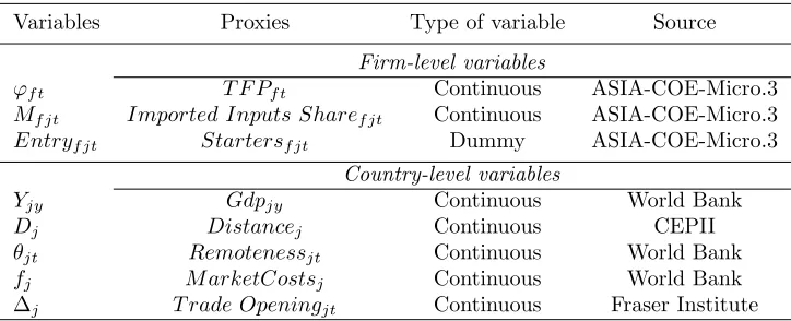
Table 2: Variables
Variables Proxies Type of variable Source
Firm-level variables
ϕf t T F Pf t Continuous ASIA-COE-Micro.3
Mf jt Imported Inputs Sharef jt Continuous ASIA-COE-Micro.3
Entryf jt Startersf jt Dummy ASIA-COE-Micro.3
Country-level variables
Yjy Gdpjy Continuous World Bank
Dj Distancej Continuous CEPII
θjt Remotenessjt Continuous World Bank
fj M arketCostsj Continuous World Bank
∆j T rade Openingjt Continuous Fraser Institute
Note: Table reports the variables used in the empirical analyses.
Starting from our database we can derive the firm-level variables used to estimate the empirical models described in Section 3.1. The top panel of Table 2 lists the firm-level variables used in the empirical analyses. To measure a firm’s productivity we use the variableT F Pf t, which is computed
as the residual of a two input (capital and labour) Cobb-Douglas production function estimated using the semi-parametric method proposed by Levinsohn and Petrin (2003). The empirical models include a variableMf jt to proxy a firm’s share of imported intermediate inputs from countryj and
its interactions with the two gravity forces. The variable Mf jt is computed as the fraction of
imported inputs from country j over the total amount of intermediate inputs of firm f, that is
Imported Inputs Sharef jt. This allows accounting for the relative importance of imports in the
total intermediate inputs of firmf.
In order to estimate equation (18) we need to single out the firms that enter into a specific export market during the period of observation. Following previous empirical studies, we define as export Starterf jt a firm that starts to export to j in t and has not exported to that destination
in the previous three years. The rationale behind this definition of trade starters stems from the empirical literature dealing with sunk costs and export market participation. Roberts and Tybout (1997) estimate that on average, in their sample of Colombian firms, after a three year absence the re-entry costs are not different from those faced by a new exporter. Due to the time span of six years, we can create three cohorts of export starters, respectively from 2001 to 2003. In total we obtain 101,064 firms that enter into a specific foreign market at a certain point in time. The number of starters is 30,415, 36,387, and 34,262, respectively for 2001, 2002 and 2003.24 As a reference group we select for each firm which is an export starter in some countries, the observations for all the other destinations in which the firm has never exported.25
3.3 Country-level data
In addition to firm-level data, we complement the analysis with information on country charac-teristics. We consider the two standard gravity-type variables, GDPjt and Distancej to proxy
for market size (Yjt) and transportation costs (Dj), respectively. Data on GDP are taken from
24Table A1 in Appendix A5 reports the number of exporter starters by country.
25In the reference group we do not include firms that are not export starters in any markets because for these firms
the dependent variable (Startersf jt) takes always the value zero. Indeed, inclusion of firm-fixed effects perfectly
the World Bank’s World Development Indicators database. Information on geographical distance comes from CEPII. Distances are calculated following the great circle formula, which uses latitudes and longitudes of the most important city (in terms of population) or of the official capital (Mayer and Zignago; 2005).
We augment the gravity model by including additional variables that might be expected to affect the costs of trading internationally. As indicated in Section 3.1 and predicted by equation (16) of our model, the probability of starting to export depends on variable trade costs not related to distance (∆j), market specific fixed costs (fj) and a multilateral resistance term (θjt). At the same
time equation (17) suggests that a firm’s export sales to a specific destination can be modelled in a parallel fashion to the model for export participation, though in this case market-specific fixed costs are not included.
For additional trade costs (∆j), we use a measure of average country-level import tariffs taken
from the Fraser Institute (T rade Openingjt).26 The market specific fixed costs (fj) can be related to
the establishment of a foreign distribution network, difficulties in enforcing contractual agreements, or the uncertainty of dealing with foreign bureaucracies. Following Bernard et al. (2011), to generate a proxy for these costs we use information from three measures from the World Bank Doing Business dataset: number of documents for importing, cost of importing and time to import (Djankov et al.; 2010). Given the high level of correlation between these variables, we use the primary factor
(M arket Costsj) derived from principal component analysis as that factor accounts for most of the
variance contained in the original indicators. Finally, to proxy the multilateral resistance terms (θjt)
we employ the variable Remotenessjt which captures the extent to which a country is separated
from other potential trade partners.27 The idea is that a remote country has high shipping costs, high import prices, and thus a high aggregate price index. As in Manova and Zhang (2012) the variable remoteness is computed for each country as the inverse of the distance weighted sum of the market sizes of all trading partners.28
The bottom panel of Table 2 lists the country level characteristics used to proxy the variables in our empirical models. After selecting the destinations for which we have the information needed to carry out our analysis, we end up with a dataset including 109 countries.29
3.4 Descriptive statistics and trends
Before moving to the econometric analyses it is useful to start with few summary statistics pointing in the direction of the linkage between importing and exporting activities.
We begin by exploring the export and import patterns of Italian manufacturing firms. Figure A1 in the appendix shows the distribution of Italian exports and imports across countries in 2003. From the figure, it turns out that although there is variation in the level of trade among countries,
26This variable is a simple average of three sub-components: revenue from trade taxes, the mean tariff rate and the
standard deviation of tariffs. Each sub-component is a standardized measure ranging from 0 to 10 which is increasing in the freedom to trade internationally. For further details see J.Gwartney, R.Lawson and J.Hall, 2012, Economic Freedom of the World - 2012 Annual Report, Fraser Institute.
27We are aware of the fact that the remoteness proxy bears little resemblance to its theoretical counterpart and
that a structural approach would be more adequate. However, in the empirical analyses our main interest lies in the elasticity of exports with respect to distance and market size. All the other country variables are simply included as controls.
28Precisely,Remoteness
j=PnGDPn∗distancenj , whereGDPnis the GDP of the origin country anddistancenj
is the distance betweennandj, and the summation is over all countries in the worldn. An alternative measure of remoteness used in Baldwin and Harrigan (2011) is given byRemotenessj=Pn(GDPn/distancenj)−1. Our results
are robust to the use of this other measure.
29The complete list of countries is reported in Table A1 in Appendix A5. Basic statistics for the different market
FRA NLD DEU GBR IRL DNK GRC PRT ESP BEL LUX ISLNOR SWE FIN LIE AUT CHE FRO AND GIBMLT TUR EST LVALTU POL CZE SVKHUN ROM BGR ALBUKR BLR MDA RUS GEO ARM AZEKAZ TKM UZBTJK KGZ SVN HRV BIHYUG MKDMAR DZALBYEGYTUN SDNMRT MLI BFA NER TCD CPV SEN GMB GNB GIN SLE LBRCIVGHA TGO BEN NGACMR CAF GNQ STPGABCOG ZAR RWA BDI SHN AGO ETH ERI DJI SOM KEN UGA TZA SYCMOZ MDG MUS COM MYT ZMBZWE MWINAMZAF BWA SWZ LSO USA CAN GRL SPMMEX BMU GTM BLZ HND SLV NIC CRI PAN AIA CUB KNA HTI BHS TCA DOM VIR ATG DMA CYM JAM LCA VCT VGB BRB MSRTTO GRD ABW ANTVENCOL GUY SUR ECUPERBRACHL BOL PRYURYARG FLK CYPLBNSYR IRQIRNISR PSE TMP JORSAU KWTBHRQATARE OMN YEM AFGPAKIND BGD MDV LKA NPL BTN MMRTHA LAO VNM KHMMYSIDN BRNPHLSGP MNG CHN PRKKOR JPN TWN HKG MAC AUS PNG NRUNZL SLB TUVNCL WLF PCN FJI VUT TON WSM MNP PYF FSM MHL ASM GUM CXR NFK COK NIU TKL 0 .05 .1 .15
Export Share by Country
0 .05 .1 .15 .2 Import Share by Country
Export and Import Share: Value
FRA NLD DEU GBR IRL DNK GRC PRT ESP BEL LUX ISL NOR SWE FIN LIE AUT CHE FRO AND MLT TUR EST LVALTU POL CZE SVK HUN ROM BGR ALB UKR BLR MDA RUS GEO ARM AZE KAZ TKM UZB TJK KGZ SVN HRV BIH YUG MKD MAR DZA TUN LBY EGY SDN MRT MLI BFA NER SEN GMB GIN SLE LBRGHACIV TGO BEN NGA CMR CAF GNQGABCOG ZAR BDI AGO ETH ERI SOM KEN UGA TZA SYCMOZ MDG MUS ZMBZWE MWI ZAF NAM SWZ USA CAN SPM MEX BMU GTM BLZ HND SLV NIC CRI PAN CUB BHS TCA DOM VIR ATG DMA JAM LCA VCT VGB BRB MSR TTO ABW ANT COL VEN GUY SUR ECUPER BRA CHL BOL PRYURY ARG CYP LBN SYR IRQ IRN ISR PSE TMP JOR SAU KWT BHR QAT ARE OMN YEM AFG PAK IND BGDLKA NPL MMR THA LAOVNM KHM IDN MYS BRN SGP PHL MNG CHN PRK KOR JPN TWN HKG MAC AUS PNG NZL TUV NCL TON COK TKL 0 .02 .04 .06
Share N.Exporting Firms by Country
0 .05 .1 .15
[image:22.612.77.548.72.245.2]Share N.Importing Firms by Country Export and Import Share: Number of firms
Figure 1: Export and Import share by country: value and number of firms. The figure reports the export and import share by country (ISO codes) in terms of value (left panel) and number of firms (right panel) for 2003. Table A1 reports the assigned official ISO code for each country.
the majority of flows are with European countries, followed by other developed markets (USA, Japan, Canada, Australia) and emerging markets (China, Brazil, Russia, Mexico, India). More importantly, the figure points toward complementarity between exporting and importing activities across countries as the areas where the majority of exports are directed to correspond to the countries where the gross of imports come from. The linkage between the two trade activities is reflected also by Figure 1 which shows the correlation between the country’s export share and the country’s import share in terms of value (left panel) and number of firms (right panel). This figure demonstrates that there is a strong positive correlation between the fraction of exports and imports at country level. To ascertain whether this correlation is related to gravity forces is the aim of our empirical analyses.
4
Results
In the next few sections, we will formally assess the fit of the model developed in Section 2 by estimating the equation for export participation (equation (18)) and that for export sales (equa-tion (19)). We will test the predic(equa-tions on the relative importance that imports have in influencing the impact of the gravity forces on the two margins of exports.
4.1 The extensive and intensive margins of exports
We start our empirical investigation by considering the probability of entry into a specific export market, that is the extensive margin. Table 3 reports the estimation results of equation (18).
Table 3: Firms’ exports extensive margin by country: the role of imports
(1) (2) (3) (4) (5) (6)
Starterf jt
lnT F Pf,t−1 0.0014*** 0.0014*** 0.0014***
(0.0003) (0.0002) (0.0002)
lnGdpjt 0.0062*** 0.0062*** 0.0062*** 0.0062*** 0.0062*** 0.0062***
(0.0005) (0.0005) (0.0005) (0.0005) (0.0005) (0.0005) lnDistancej -0.0094*** -0.0093*** -0.0093*** -0.0093*** -0.0093*** -0.0093***
(0.0014) (0.0014) (0.0014) (0.0014) (0.0014) (0.0014) lnRemotenessjt 0.0057 0.0057 0.0057 0.0056 0.0056 0.0056
(0.0042) (0.0042) (0.0042) (0.0042) (0.0042) (0.0042) M arketCostsj -0.0014** -0.0014** -0.0014** -0.0014** -0.0014** -0.0014**
(0.0007) (0.0007) (0.0007) (0.0007) (0.0007) (0.0007) T rade Openingjt 0.0006 0.0006 0.0006 0.0005 0.0005 0.0005
(0.0004) (0.0004) (0.0004) (0.0004) (0.0004) (0.0004) Imported Inputs Sharef jt 0.2196*** 0.1704 0.2162*** 0.1696
(0.0271) (0.5193) (0.0269) (0.5230)
∗lnGdpjt 0.0282* 0.0280*
(0.0155) (0.0156)
∗lnDistancejt -0.0885*** -0.0882***
(0.0268) (0.0269)
Year FE Yes Yes Yes
Firm FE Yes Yes Yes
Firm-Year FE Yes Yes Yes
Adj. R2 0.034 0.038 0.038 0.052 0.052 0.052
N.Observations 7,055,819 7,055,819 7,055,819 7,055,819 7,055,819 7,055,819
Note: The table reports regressions using data on 1998-2003. The dependent variable used is reported at the top of the columns. All the regressions include a constant term. Regressions are run on the same observations in all specifications. Robust standard errors clustered at country level are reported in parenthesis below the coefficients. Asterisks denote significance levels (***:p<1%; **: p<5%; *: p<10%).
of exporting.30 We cluster standard errors at the country level in order to allow for correlation of the error terms across firms for a given destination.31
We start in column 1 of Table 3 by reporting the results of a model without considering the import status of a firm and controlling for firm and year fixed effects. The results provide a clear picture. The productivity variable has the expected positive and significant sign: a positive firm-level productivity shock at time t increases the likelihood of starting to export to a specific country at time t+ 1. Specifically, a 10 percent increase in firm productivity is associated with an increase of about 0.014 percentage points in the probability of exporting. The magnitude of this effect is sizeable (i.e., 1%) if compared with the probability of starting to export observed in our sample, which is 0.014. As for the two gravity variables, we find that the probability of entry into a specific market increases with market size but decreases with distance. A 10 percent rise in the destination country’s GDP is associated with an increase of 0.062 percentage points in the probability of starting to export to that country. A 10 percent increase in distance decreases the
30As a robustness check, we perform a validation exercise where we explore results under a different definition of
export starters. The variableEntrytakes value 1 if a firm starts to export to jintand has not exported to that destination in the previous two years. The results are robust to this alternative definition and are available upon request.
31Our results are robust to alternative treatments of the error terms, such as clustering by firm or firm and country.