High Performance Implementation of Support Vector Machines Using OpenCL

(1)

Theses Thesis/Dissertation Collections

5-2014

High Performance Implementation of Support

Vector Machines Using OpenCL

Ethan Peters

Follow this and additional works at:http://scholarworks.rit.edu/theses

This Thesis is brought to you for free and open access by the Thesis/Dissertation Collections at RIT Scholar Works. It has been accepted for inclusion in Theses by an authorized administrator of RIT Scholar Works. For more information, please [email protected].

Recommended Citation

(2)

Vector Machines Using OpenCL

by

Ethan Peters

A Thesis Submitted in Partial Fulfillment of the Requirements for the Degree of Master of Science

in Computer Engineering

Supervised by

Professor Dr. Andreas Savakis Department of Computer Engineering

Kate Gleason College of Engineering Rochester Institute of Technology

Rochester, New York May 2014

Approved by:

Dr. Andreas Savakis, Professor

Thesis Advisor, Department of Computer Engineering

Dr. Muhammad Shaaban, Associate Professor

Committee Member, Department of Computer Engineering

Dr. Sonia Lopez Alarcon, Assistant Professor

(3)

Rochester Institute of Technology Kate Gleason College of Engineering

Title:

High Performance Implementations of Support Vector Machines Using OpenCL on Heterogeneous Systems

I, Ethan Peters, hereby grant permission to the Wallace Memorial Library to reproduce my thesis in whole or part.

Ethan Peters

(4)

Dedication

This thesis is dedicated to my wife Cassandra Madison-Peters, without whose encouragement this work would not have been possible. I would also like to dedicate this

work to my family, who have supported me throughout my academic career. Finally, I dedicate this work to my colleagues and professors, who have been instrumental in my

(5)

Acknowledgments

I would like to thank Dr. Savakis for all of his guidance and help on this research. I would also like to thank the members of my committee, Dr. Shaaban and Dr. Lopez Alarcon, for their feedback and assistance to my work. Finally, I would like to thank my colleagues Riti Sharma and Breton Minnehan for sharing their knowledge with me, and Jack Stokes

(6)

Abstract

High Performance Implementation of Support Vector Machines Using OpenCL

Ethan Peters

Supervising Professor: Dr. Andreas Savakis

Support Vector Machines are a machine learning approach that is well studied,

thor-oughly vetted and effective in a large number of applications. The objective of this thesis is

to accelerate an implementation of Support Vector Machines (SVM) using a heterogeneous

computing system programmed using OpenCL in C/C++. LIBSVM, a widely-available,

popular and open source implementation of SVM is chosen, allowing the presented work

to be integrated seamlessly into existing systems. The proposed framework is evaluated in

terms of speed and accuracy when performing training and classification on a number of

standard data sets. Testing was based on two work station GPUs, the NVIDIA GTX 480

and Tesla K20, and a modern, work station CPU (Intel i5 Quad Core, 3 GHz).

We find that, for large data sets, training is accelerated by a factor ranging from 9 to 22.

In general, speedup increases with the total number of training samples in the data set until

the GPU device is fully utilized. While these gains in speedup are significant, they do not

match the ideal parallel speedup, that is the total number of cores in the parallel system.

Our findings indicate that performance is hampered by the portions of the SVM training

algorithm that are sequential. In addition, we find that the classification phase of the SVM

system is accelerated by a factor of up to 12. During classification only a relatively small

(7)

the computational complexity of classification grows only linearly with the number of

sam-ples processed, as opposed to the training phase where it grows quadratically. The

contri-butions of this thesis include the use of OpenCL for accelerating SVM training and testing

(8)

List of Figures

2.1 SVMs seek to find a hyerplane which maximizes margin between two classes 8

2.2 SVM Formulations Offered by LIBSVM . . . 18

2.3 SVM Kernels Offered by LIBSVM . . . 18

2.4 LIBSVM Algorithm Flowchart . . . 20

3.1 OpenCL Platform Model . . . 23

4.1 Illustration of Matrix-Vector Multiplication . . . 31

4.2 Parallelization of Matrix-Vector Multiplication. Colors indicate division of labor amongst work groups . . . 31

4.3 Illustration of Dot Product Parallalization. Colors indicate division of labor amongst threads. . . 31

4.4 LIBSVM Algorithm Flowchart . . . 36

4.5 Kernel Matrix Row Calculation Flowchart . . . 37

4.6 Kernel Matrix Row Calculation Flowchart . . . 37

4.7 Kernel Matrix Calculation Flowchart . . . 38

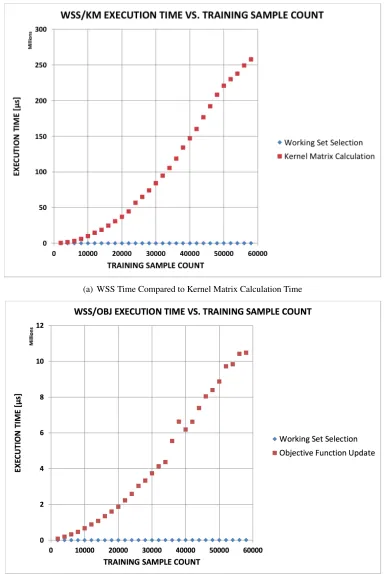
5.1 Working Set Selection Comparison . . . 47

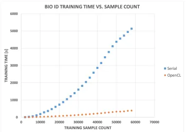
5.2 BIO ID Raw Image Training Performance (GTX 480) . . . 49

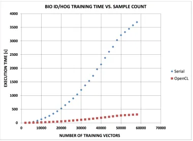
5.3 BIO ID HOG Training Performance (GTX 480) . . . 50

5.4 BIO ID HOG Training Performance Across GPUs . . . 51

5.5 PASCAL VOC Training Performance (GTX 480) . . . 53

5.6 PASCAL VOC Training Perform Across GPUs . . . 54

5.7 BIO ID Raw Image Training Performance (Non-Linear Kernels) (GTX 480) 56 5.8 BIO ID Raw Image Training Performance (Non-Linear Kernels) (GTX 480) 57 5.9 BIO ID HOG Training Performance (Non-Linear Kernels) (GTX 480) . . . 60

5.10 BIO ID HOG Training Performance (Non-Linear Kernels) (GTX 480) . . . 61

5.11 BIO ID HOG Training Performance (Non-Linear Kernels) On All GPUs . . 62

5.12 BIO ID HOG Training Performance (Non-Linear Kernels) Across GPUs . . 63

5.13 Speedups for All Training Kernels On All Available GPU Devices . . . 64

5.14 Objective Function Calculation Performance Breakdown . . . 65

(11)

5.16 Kernel Matrix Calculation Performance Breakdown (GTX 480) . . . 67 5.17 Effort Comparison (GTX 480) . . . 68 5.18 BIO ID Raw Image Classification Performance (GTX 480) . . . 72 5.19 BIO ID Raw Image Classification Performance (Non-Linear Kernels) (GTX

480) . . . 73 5.20 BIO ID Raw Image Classification Performance (Non-Linear Kernels) (GTX

480) . . . 74 5.21 Error in Alpha Vector from Reference for Models Trained on BIO ID Data

(12)

Chapter 1

Background

1.1

Computer Vison

Computer vision deals with interpreting image data and obtaining an understanding of

the depicted scene or object. It is an important pursuit for fields including artificial

intelli-gence, robotics and human-computer interaction.

Parallel processing systems present major performance improvements for algorithms

which are well suited to them. They are of particular interest for image processing

applica-tions, as most such algorithms have a high degree of inherent parallelism; that is to say they

are well suited to being performed on parallel processing systems because they involve a

large number of independent (typically light-weight) operations. For instance, in pixel and

neighborhood processing algorithms, each output pixel value can be computed

simultane-ously by performing a relatively simple operation on a small amount of input data. Such

systems can be made to scale well with the size of input data, because the computation time

of such a parallel algorithm decreases linearly with the number of computing elements in

the system, often without the need for individual computing elements to become

signifi-cantly more sophisticated (and consequently more costly).

A Graphics Processing Unit (GPU) is a computational device that typically serves as the

processing engine of a larger graphics processing system. These systems were originally

(13)

systems designed for processing computer generated images (such as video game systems

and 3D animation work stations). To benefit this specialized task, GPUs are designed to be

low-cost, highly parallel processing systems, employing a large (and growing) collection

of relatively weak cores. These characteristics make the GPU an attractive platform for

applications with inherent parallelism, such as image processing, and so General Purpose

computing on a GPU (GPGPU) has drawn a large amount of interest in recent years.

In addition to providing a low-cost parallel system, many image processing algorithms

don’t suffer from the inherent weakness of each individual core, as the tasks to be

per-formed are light weight and involve small amounts of data, therefore GPUs provide a

plat-form which very closely matches many of the work loads encountered. This close match

between the requirements of these algorithms and the benefits offered by GPUs means that

in many cases they provide the optimal tradeoff between cost and performance. Even in

situations where a GPU is not sufficient for the final intended application of a system, it

can still prove useful as a testbed for a new parallel algorithm or data access model.

GPUs are not without their drawbacks, however. Standard processing cores are not

typ-ically used in graphics systems (for cost and chip resource reasons), thus GPUs present

a specialized programming environment which requires a greater effort on the part of the

programmer. Furthermore, manufacturers of GPUs adhere to different standards, not only

for individual processing units but for the interconnect and command structure of the chip

as well, meaning that each GPU is a different, specialized programming environment.

1.2

Heterogeneous System Architecture

Heterogeneous Computing (HC) refers to computing systems that not only use

multi-ple computational elements, but elements of different types. Computing elements can vary

widely in their internal structure and intended task, and consequently a single algorithm can

have different performance implications depending on the platform on which it is run and

(14)

have hundreds of processing cores, making them a good target platform for tasks requiring

small, independent computations; however, these cores tend to be relatively weak, so a task

that is inherently serial (requiring a long chain of operations to be performed in sequence)

and generally intensive (such as floating point arithmetic) would be a poor fit for a GPU

and a much better fit for a traditional CPU.

Additionally, NVIDIA GPUs make use of a VLIW type of instruction dispatch, where

some number of instructions are dispatched in parallel to a single group, or warp, of cores.

For Kepler architectures, two independent instructions can be dispatched to 32 cores at

once[43]; this is a highly restrictive form of parallelism, thus an algorithm must be highly

conducive to GPU acceleration for its benefits to overcome its drawbacks.

We can take advantage of this kind of system by segmenting the algorithm being

imple-mented into separate algorithms based on the level and type of parallelism present in each

part; then these separate algorithms are mapped onto and optimized for the available

hard-ware that best meets their needs. Desktop work stations can be a good gateway into larger,

more complete heterogeneous systems because modern work stations typically contain a

multicore CPU, a discrete graphics card and an integrated GPU living on the same die as

the CPU.

A multicore CPU, which is itself a traditional parallel processing system containing a

limited number of very powerful cores, is extremely well suited to serial operations;

indi-vidual CPU cores benefit from decades of research and development into optimizing their

performance on traditional, serial operations, and include physical constructs that

imple-ment optimizations such as high accuracy branch prediction, deep pipelining, dependency

resolution, multi-level caching and prefetching, and hardware conducive to instruction level

parallelism such as reservation stations (to avoid having to share registers between

unre-lated operations) and redundant operative elements such as ALUs and FPUs (to allow

un-related operations to take place simultaneously).

(15)

large die area and thus there are limitations on the number that can be fit onto a single chip.

While these limitations can be accomodated to some degree by connecting large numbers

of chips together in larger systems, cooperation between computational cores becomes

dif-ficult and costly across chip boundaries, while increasing the area of chip tends to decrease

the yield of the process (or increase the likelihood that any single chip produced will be

faulty and unusable); that is not to say that these systems can not be effectively applied to

parallel problems (indeed, there is definitive proof that they can), but rather that the types

and scale of parallel problems for which these kinds of system are optimal is limited by the

cost of coordination and communication across chip boundaries, in addition to the cost in

power of many-core chips and the monetary cost of fabricating more complex chips.

Discrete GPU devices, which contain a large number of weak cores, offer a different

approach; individual GPU cores forego complex hardware constructs typical of standard

CPU cores in favor of being small enough to fit tens or hundreds of cores onto a single die.

Consequently, discrete graphics cards allow more tasks to be more closely coordinated at a

reduced communication cost, at the expense of instruction level parallelism, since

individ-ual cores have only a limited capacity for computation.

Desktop workstations also often contain, as a bonus, GPUs integrated onto CPU core

dies; such a GPU has fewer cores than a discrete GPU but has access to system memory

and requires less overhead for coordination with the rest of the system. Integrated GPUs

can communicate using the system bus, compared to discrete GPU devices which connects

to a computer’s motherboard using PCI, or something similar, which presents significant

overhead for communicating between computational devices.

The term Heterogeneous System Architecture is also applied to the design of integrated

circuits consisting of tightly coupled heterogeneous computing units, the terms ”system”

and ”architecture” being relatively flexible. For clarity, it is emphasized that this thesis

does not present a hardware implementation, specification or design and the terms ”HSA”

(16)

that are design to operate in a hetereogeneous environment.

1.3

OpenCL

OpenCL (Open Computing Language) is a software platform designed to provide a

consistent interface for programming computational devices for specialized hardware such

as GPUs, Field Programmable Gate Array (FPGA) platforms, certain CPUs, etc. It is an

open specification maintained by the Khronos Group, and it allows software written in a

standard, familiar programming language (C99) to run on any of the devices supported,

with an emphasis on parallel computation. It is of particular interest to developers working

on GPGPU applications, because OpenCL works across all of the major GPU hardware

vendors and doesn’t require learning a new programming lanugage for each target device.

More importantly, however, is that OpenCL allows one’s application to work across a

generalized, heterogeneous computing system. That is, OpenCL applications can make use

of systems with many different types of computational devices. It allows this by first its

ability to run on almost any major computational device, and second by providing utilities

for an application to understand what hardware is available and to adjust task allocation

across devices to best make use of the available hardware.

Having discussed the general means by which HC is applied to accelerate computation,

in the next section (and the chapter following), we consider a particular application which is

well suited to, and in serious need of the advantages described. Namely, the algorithms used

in constructing and using Support Vector Machines, and their applications, are presented.

1.4

Support Vector Machines

Support Vector Machines (SVMs) are a particular style of machine learning algorithm

commonly used in computer vision problems. SVMs operate in two phases: training and

(17)

to which it belongs; SVMs treat all data as vectors or points in some (potentially) high

dimensional space. Traditionally, an SVM is used to distinguish between two classes of

objects, so two labels are accepted. The algorithm then attempts to find a hyperplane that

separates the two classes by maximizing the margin between the classes. During

classi-fication, the trained SVM identifies the class to which a point belongs by determining on

which side of the plane the point lies.

1.5

Thesis Overview

In this thesis we contribute the following items: first, an accelerated implementation

of LIBSVM, a popular and powerful library for machine learning, which is reasonably

easily to use optimally on a variety of hardware and reasonably easy to use in place of the

original; secondly, a case study in HC acceleration using the OpenCL platform. The work

is laid out as follows: in the following chapter, we discuss the particular set of algorithms

(namely those used in SVM) we are attempting to optimize; the next chapter presents our

plans for optimization of the algorithms discussed; in the chapter which follows we present

the experiments we have conducted as well as the results we have obtained and we draw

general conclusions from them; finally we present a summary of our work, its meaning and

(18)

Chapter 2

Support Vector Machines

The Support Vector Machine (SVM) is a type of machine learning algorithm for

bi-nary (two class) classification problems, discussed at length in [2] and [17]. SVMs operate

in two phases: a training phase, in which labeled data is used to build an SVM model,

and a classification phase, during which the trained model is used to determine the class

where some new set of data belongs. SVMs work by viewing input data as vectors, and

consequently points in some high dimensional space. During training, the SVM finds a

hyperplane which separates the labeled training data into distinct classes based on a

maxi-mum margin criteria. During classification, the SVM calculates where new data points lie

with respect to this hyperplane using a decision function outlined below.

D(~x) =w~ ·~x+b (2.1)

where,~xis the new data vector being classified, andw~ andbare a vector and a scalar,

respectively, which are learned during training and describe the separating hyperplane. This

function relates to the distance between ~xand the hyperplane, and consequently the sign

ofD(~x)will determine to which class the point belongs.

It is not always possible to separate the training data using a linear hyperplane; for

in-stance, positive samples may cluster around a single point, with negative samples scattered

(19)

[image:19.612.232.395.92.181.2]

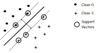
Figure 2.1: SVMs seek to find a hyerplane which maximizes margin between two classes

However, for many data sets it may be possible to find some other shape to separate the

data; that is, a hyperplane in some non-linear space may be ideal for these data sets. To do

this, a kernel is introduced that maps input data into some space that is more conducive to

separating the data, which manifests in the decision function as follows.

D(~x) = w~ ·φ(~x) +b (2.2)

The actual Euclidian distance between the given data point,~x, and the SVM’s

charac-teristic hyperplane can be expressed as

d(~x) = D(~x)

||w~|| (2.3)

An SVM model is in part characterized by its margin; that is, the distance from the

hyperplane to the nearest points in the training set.

M =min k

~

y_kD(x~k)

||w~|| (2.4)

Here, yk are data point labels, indicating negative or positive samples. A good SVM

classifier seeks to create as much separation between the two classes as possible to reduce

the possibility of confusing points that are near the class boundary. The approach presented

(20)

the supporting vectors. This goal is expressed in the optimization problem below. max ~ w min k ~

y_kD(x~k)

||w~||

(2.5)

Here,y~_k=±1is the class corresponding to the vectorx~k. The constraint is added that

M||w~||= 1 to restrict the problem space from an infinite number of possible solutions to

a single feasible solution, and consequently the problem becomes

min

~

w ||w~||

2 _(2.6)

subject to

~

y_kD(x~k)≥1∀k (2.7)

This problem is theoretically solvable, but it is computationally impractical when the

dimensionality of w~ becomes very high. For this reason, the Lagrangian of the

prob-lem is taken and the dual space optimization probprob-lem is formed, as per work presented in

[19][20][21].

The Lagrangian of the problem is

L(w, b,~ α~) = 1 2||w~||

2₋X

k ~

αk[~ykD(x~k)−1] (2.8)

whereα~k are the Lagrange multipliers and together form a vector α~. At the solution,

the following condition holds

dL

dw~ =w~ − X

k ~

αk~ykφ(x~k) = 0 (2.9)

~

w=X

k ~

(21)

As per [2], the solution to this problem should be a maximum ofL(α, b, w)with respect

toα. We reformulate the term in the above equation that depends onα.

X

k ~

αk[~ykD(x~k)−1] =

X

k ~

αk~ykD(x~k)−

X

k ~

αk (2.11)

=X

k ~

αk~yk(w~ ·φ(x~k) +b)−

X

k ~

αk (2.12)

We can substitute into the above equation to get an equation in terms ofα. Additionally,

we set the offsetbto zero and solve for it later.

X

k ~

αk~yk(w·φ(x~k) +b)−

X

k ~ αk =

X

k ~ αk~yk

X

z ~

αz~yzφ(x~z)

!

φ(x~k)

! −X k ~ αk (2.13)

By expanding vector operations we can rewrite the above

X

k ~ αk~yk

X

i X

z ~

αz~yzφi(x~z)φi(x~k)

!

−X

k ~

αk (2.14)

=X k ~ αk X i X z

[~y_z~y_kφi(x~z)φi(x~k)]α~z− X

k ~

αk (2.15)

whereφi(~x)is theith element in the vectorφ(~x). Finally, we reformulate this into its

final representation.

min

~

α (f(α~)) (2.16)

f(α~) = 1

2αQ~~ α−

X

k ~

αk (2.17)

~ wi =

X

k ~

αkφi(x~k) (2.18)

Qis the kernel matrix:

(22)

The label factors are often omitted in this work because their product calculation is trivial

and can be circumvented using flow control.

In this problem domain, values of a kernel functionK(x, y)are chosen such that

K(~x,y~) =X

i

φi(~x)φi(~y) (2.20)

With these definitions, the decision function can be rewritten in terms ofα~.

D(~x) = X

k ~

αkK(x~k,~x) +b (2.21)

Here,x~k is thekthsupport vector and~xis the vector being classified.

Sequential Minimal Optimization

Platt et. al. [4] present a simple, efficient and effective technique for finding the

op-timal α~ vector for Support Vector Machines that has become the basis for popular SVM

implementations, called Sequential Minimal Optimization (SMO). The basic tenet of this

approach is to break down the large optimization problem presented into the smallest

pos-sible optimization problem, that is solving for two elements of α~, and repeating this

op-timization until the entire vector is optimized. In this way, the inner loop of the SMO

algorithm is a single calculation, rather than an optimization problem itself. There are

three phases in the SMO algorithm as described by Platt:

1. Check for Terminating Conditions

2. Select Working Set

3. Optimize Working Set

Also worth noting is that SMO actually attempts to solve a slightly modified version

off(α~), introduced in [5]; it introduces a tolerance term that allows some adjustable

(23)

in cases when the training samples are not linearly separable.

min

~ w,b,ζ

1 2||w~||

2₊_CX

i

ζi (2.22)

This extra term leads to another constraint in the dual space.

0≤α~k≤C ∀k (2.23)

Terminating Conditions

The Karush-Kuhn-Tucker (KKT) [35] conditions for optimality dictate that α~ is an

optimal solution off(α~)if and only if there exist values which satisfy

∇f(α~) +b~y =~λ−~ζ (2.24)

~

λiα~i = 0,ζ~i(C−α~i) = 0,~λi ≥0,~ζi ≥0,∀i (2.25)

We can rewrite this equation.

∇if(α~) +b~yi =  



≥0 : ~αi < C,

≤0 : ~αi >0

(2.26)

Sincey=±1, we know thatbis constrained within a range.

max i∈Iup

−~y_i∇if(α~)≤b ≤ min i∈Idown

−~y_i∇if(α~) (2.27)

Iup(α~) ={t|α~t< C,~yt= 1or ~αt >0,~yt=−1} (2.28)

Idown(α~) ={t|~αt< C,~yt=−1or ~αt >0,~yt= 1} (2.29)

Once the two values are sufficiently close, b is calculated as their average, the KKT

(24)

a vector of all ones and updated at each iteration according to

∇f(α~)r+1 =∇f(~α)r+1+ ∆α~iQi+ ∆α~jQj (2.30)

Here, ∆α~i is the amount by which the selected α component has changed andQ~i is

a column of the kernel matrix. In this way, ∇f(~α) = αQ~ −~e is maintained. Here~e

is a vector of all 1. It is worth noting here that this formula is a vector addition and can

potentially be of very high degree; this makes this step in the operation a good candidate

for parallelization, since vector additions contain a large number of simple, completely

independent operations which all rely on data that exhibits spatial locality and is thus cache

friendly (meaning that only the first set of accesses will suffer full communication penalty).

Working Set Selection

The next step in the algorithm is to select the indices ofα~ to optimize in this iteration.

Since the algorithm can finish when the KKT conditions are met, it makes sense to select

the two values which most violate these conditions, and in fact this is the initial proposal

by Platt. However, [6] presents an optimization which uses second order information to

converge in fewer iterations.

As shown in equation 2.27,bis bounded.

m(~α)≤b≤M(α~) (2.31)

m(~α) = max i∈Iup

−~y_i∇if(α~) (2.32)

M(α~) = min i∈Idown

−y~_i∇if(α~) (2.33)

We first select the indexithat definesm(α~).

i∈arg max

t {−~yt∇f(α~ r

(25)

Then we select a value ofj which definesM(α~); should this value exceedm(α~), this

is a violating pair which should be the next to be optimized.

j ∈arg min

t {−~yt∇f(α~ r

)t|t∈Ilow(α~r)} (2.35)

As [6] points out, this is equivalent to trying to minimize a first order approximation of

fα~r+d~≈f(α~r) +∇f(α~r)T d~ (2.36)

whered~is the change inα~. The optimization proposed in [6] is to make this

minimiza-tion of a second order approximaminimiza-tion.

f~αr+d~−f(~αr) = ∇f(α~r)T d~+1 2

~

dT∇2_f₍_α_~r

)d~ (2.37)

Therefore, we select i as above, and then select j to minimize this function.

j ∈arg min

t {Sub({i, t})|t∈Idown(α~ r

),−~y_t∇f(α~r)t <−y~i∇f(α~ r

)i} (2.38)

Sub(B) =min

~ d

∇f(α~r)T d~+1 2d~

T

∇2_f₍_α_~r

)d~ (2.39)

Theorem 3 in [6] states that, as long as{i, j}form a violating pair, this function has an

optimal value at

−

−y~_i∇f(α~r)_i+~y_j∇f(α~r)_j

2

2 (Kii+Kjj −2Kij)

(2.40)

Therefore, we select the working set as follows.

j ∈arg min t

−b

2 ij

a∗_ij|t∈Idown(α~ r

),−y~_t∇f(α~r)t<−y~i∇f(α~ r

)i

(2.41)

(26)

a∗_ij =

 



aij if aij >0

τ otherwise

(2.43)

bij =−∇if(α~k) +∇jf(α~k) (2.44)

Note that in this kind of minimization problem, with large computations being

opti-mized over a single value, we can parallelize this by computing the function for all values

of t first, and then simply traversing the resulting data linearly (and quickly) to find the

smallest value. This can further be parallelized by doing a tree based reduction of the data

to find the minimum; that is, break the data into sets of two elements and find the

maxi-mum of each set simultaneously, then repeat on the remaining data set until the maximaxi-mum

is found. This allows all of the computational elements to be applied to the operation and

reduces the running time logarithmically.

Minimal Optimization

Finally, to optimize the selected working set, the previous optimization problem is

ap-proached, but is constrained to only two variables.

min

~ αi,α~j

1

2[~αi α~j]





Q_ii Q_ij

Q_ji Q_jj     ~ αi ~ αj 

+ (Q_iα~ + 1)α~i+ (Qj~α+ 1)α~j (2.45)

From this equation, the derivative is extracted and set to zero, then the components can be

solved. Here,N represents

~

αnew_i =α~k_i +y~_ibij

a∗_ij (2.46)

~

αnew_j =α~k_j −~y_ibij

a∗_ij (2.47)

Following this solution, the new values ofα~ are then constrained such that

(27)

and

~

αr_i+1−α~r_j+1 =α~r_i −α~r_j (2.49)

To do this, if one of the new components ofα~ falls outside of this range, it is clipped

(that is, constrained to the bound it violates) and the other component is adjusted to

main-tain that the difference between the components has not changed. For instance, ifα~r_i−α~r_j >

Ci−Cj andα~ir+1 > Ci, we setα~ri+1 =Ci,~αrj+1 =Ci−(α~ri −~α r j).

In this phase, as in other phases, the kernel matrixQneeds to be calculated by

perform-ing a high dimensional matrix vector multiplication operation. These are highly parallel

operations, since they require a large number of inner products to be calculated (two

ele-ment multiplications en masse followed by reductive additions). Furthermore, for reasons

discussed later, calculating the kernel matrix requires an extra phase of operation that is

entirely element-wise.

2.1

SVM Applications in Computer Vision

Support Vector Machines have been applied successfully to a number of machine

learning problems. [10] uses both polynomial and radial basis function kernel SVMs to

recognize handwritten text in images; here, SVM is chosen in part because the data used

is linearly separable and sparse but comes in large quantities of training vectors. An

im-plementation called svmlight is used and the two kernels used achieve 86 and 86.4 percent

accuracy respectively. In [11], a soft margin version of SVM is also used in text

classifi-cation and compared to a number of neural network based approaches. The work done in

[39] uses directional element features to apply SVMs to classification of Chinese

charac-ters, along with a coarse-to-fine approach. They achieve 100% classification accuracy for

(28)

SVMs are commonly used for face detection [26][25] and other human feature

detec-tion [24][22][23]. The work done in [12] applies a custom method for performing SVM

training to the task of face detection in images. They achieve a correct detection rate of 97

percent for certain test data sets.

Sharma and Savakis, in [13], use LIBSVM, a common implementation of SVM, to

classify images using a descriptor based approach. Their system uses a Histogram of

Ori-ented Gradients (HOG) descriptor to extract significant features from eye images, and then

performs Principal Component Analysis (PCA) on the resulting HOG descriptors. The

re-sultant data is used to train an SVM model, and then this model is used to classify eye

images with accuracies exceeding 98 percent. This illustrates the effectiveness and

flexi-bility of an SVM- based approach.

In [37], SVMs are applied to computer aided diagnosis. Specifically, the work uses

a custom formulation of an SVM in order to detect microcalcifications in mammogram

images. The custom formulation is called a tangent vector SVM (TV-SVM) meant to

in-troduce rotation invariance, since microcalcification clusters do not vary in their properties

with their orientation.

In [38], a multiresolution approach is taken to classify hyperspectral images. They

per-form wavelet decomposition on the images being tested, then perper-form classification on the

lower resolution images first. This allows them to eliminate images before much effort is

invested in their classification, reducing the computational effort of SVM classification.

An interesting application of SVM is [40]; images of olive oil samples are taken in

mul-tiple color spaces, used to form histograms and converted to a lower dimensionality using

PCA. Then the resultant description of each image sample is run through an SVM to

de-termine its impurity level. This is a multiclass SVM problem, as samples were grouped as

“low impurity level”, “acceptable impurity level” or “unacceptable impurity level”; using

(29)

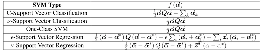
SVM Type f(~α)

C-Support Vector Classification 1₂αQ~~ α−P

kα~k

ν-Support Vector Classification 1₂αQ~~ α

One-Class SVM 1₂αQ~~ α

-Support Vector Regression 1₂(~α−α~∗)Q(α~ −α~∗)−P

i(α~i+~α∗i) +

P

i~zi(α~i−α~∗i) ν-Support Vector Regression 1₂(α~ −α~∗)Q(α~ −α~∗) +~zT (α−α∗)

Figure 2.2: SVM Formulations Offered by LIBSVM

Kernel Name K(~x,y~)

Linear ~x·~y

Polynomial (~x·~y+c)d RBF e−γ||~x−~y||2

[image:29.612.88.537.88.175.2]

Sigmoid tanh(~x·~y+c)

Figure 2.3: SVM Kernels Offered by LIBSVM

2.2

LIBSVM

The central SVM engine used in this work is LIBSVM, introduced in [3]. It is a

pow-erful, open source, widely available and thoroughly vetted system that offers very thorough

support for SVM. It is popular among research groups because, being open source and

reliably hosted, it is easy to access and use LIBSVM and thus gain the benefits of SVM

without the need to understand its inner workings. Furthermore, LIBSVM’s feature set is

broad enough, and its interface flexible enough, that it can be easily applied to a broad range

of applications. Additionally, because LIBSVM is open source, it is a popular platform for

experimenting with enhancements to SVM algorithms.

LIBSVM supports five basic configurations of SVM, both for training and

classifica-tion, listed by the table in Figure 2.2. In addiclassifica-tion, LIBSVM supports the use of four kernel

functions, defined in Figure 2.3. LIBSVM also supports a precomputed kernel function,

allowing the user to supply kernel values within the training data.

LIBSVM has three primary external interfaces; there is an application programming

in-terface (API), written in C/C++, that exposes a flexible set of SVM primitives that are easy

(30)

of command line tools for training and classification built around the C/C++ API. This is

likely the easiest interface to use as it requires no programming, and training and

classifica-tion tools both produce and consume data files which are easy to interpret and parse using

the C/C++ API in a custom application. Finally, there is a MATLAB interface, also built

around the C/C++ interface, that makes the basic API available in MATLAB through mex

files, ensuring they are as performant as possible while maintaining a consistent interface

with the other approaches. This is an important addition as MATLAB is often an optimal

programming environment for research groups, especially those where extensive

program-ming experience is not common, or when speed of development is of great importance.

LIBSVM makes use of an SMO type algorithm, as introduced in the previous section,

including the discussed optimization to the working set selection step. However, the library

adds some optimizations to reduce the computational load of the approach. In particular,

the library uses a shrinking technique, introduced in [15] and discussed at length in [14].

The general premise of this approach is that if certain components of the vectorα are not

changed over a large number of iterations, they are unlikely to be changed at any point in

future iterations of the SMO algorithm; consequently, if certain indices can be proved to

be stable they can be removed from consideration for the working set selection step, which

can reduce the computational effort of the entire algorithm.

Work done in [16] and [14] show formal proofs that, under certain working set

selec-tion algorithms, during the final iteraselec-tions of the SMO algorithm only a small subset of the

vectorαis updated. Another logical consequence of this is that only a small subset of the

kernel matrixQis used during these iterations; this reduced set is likely small enough to fit

into the system’s memory, and so LIBSVM employs a caching technique that saves values

ofQij for future use.

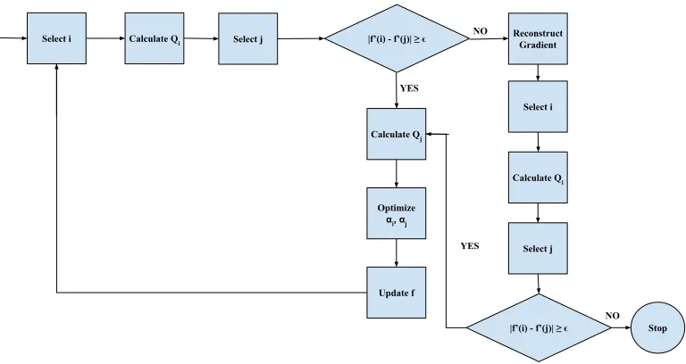
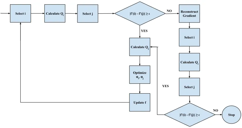
For clarity, 2.4 shows an overview of the SMO algorithm is implemented in the

(31)

Select i Calculate Qi Select j |f’(i) - f’(j)| ≥ ϵ

NO Reconstruct Gradient

Select i

Calculate Qi

Select j

|f’(i) - f’(j)| ≥ ϵ NO

Stop YES

Calculate Q_j

Optimize

αi, αj

Update f

[image:31.612.119.503.92.296.2]

YES

Figure 2.4: LIBSVM Algorithm Flowchart

2.3

GPU Assisted LIBSVM

This thesis will be influenced by the work done in [8], which is a GPU

acceler-ated SVM implementation using the CUDA framework (GPU LIBSVM). It is based on

LIBSVM and is an extension on the existing code base, slightly stripped down for focus,

implementing only the SVM core and the SVM training command line module. This

sys-tem uses a GPU to accelerate the calculation of the radial basis function kernel during the

cross validation phase of training. Cross validation is a technique used to heuristically find

the optimal value for C, the factor that dictates leniency in the constraint that all training

samples be cleanly separated by the SVM’s characteristic hyperplane. The work done in

[8] also introduces a new internal data format for the training vectors used by LIBSVM

that is more conducive to intersystem communication; the work presented here uses this

format.

There are two limitations in the work in [8] that this work attempts to overcome; the first

is that its domain is narrow, accelerating only one kernel (the radial basis function kernel)

(32)

to CUDA systems; this is considered a weakness here because it potentially eliminates a

wide range of computationally powerful devices from being utilized.

The work presented in [8] is based on cuSVM, introduced in [7], itself a GPU-based,

accelerated version of SVM-based loosely on LIBSVM. CuSVM uses the same general

algorithms as LIBSVM, but is largely rewritten in C/C++, using CUDA, designed to

inter-face with MATLAB. Because of the nature of the rewrite, cuSVM is only accessible using

MATLAB and thus loses a large portion of its utility and accessibility. Furthermore, it is

(33)

Chapter 3

OpenCL

This thesis will make use of OpenCL, the Open Compute Language, which is a

col-lection of libraries that together form a platform for Hetereogeneous Computing System

design. OpenCL allows any C/C++ program to interface with parallel computation

de-vices, including GPUs, FPGAs, parallel CPUs and even specific accelerators such as the

IBM CELL Blade [9]. OpenCL is supported by GPU devices that support the CUDA

framework, as well as a number of AMD and ATI GPUs and AMD and Intel CPUs, and

even some ARM CPUs, such as some of those provided by Qualcomm [41].

OpenCL primarily supports a data parallel programming model, wherein the same

com-putation is applied to several memory elements in parallel. The main element of

compu-tation is referred to in OpenCL as the kernel (not to be confused with the SVM kernel

function), and its code is compiled using the OpenCL compiler in a subset of C99 which is

extended to allow for certain vector operations. The language also provides certain C

stan-dard library operations such as exponential calculation and some trigonometry functions.

Kernels are executed in local work groups, which provide the perception of being executed

in parallel all at once, thus allowing synchronization between threads; a single work group

is therefore ideal for parts of the kernel requiring synchronization.

Local work groups are joined together to form a global work group which defines the

(34)

Figure 3.1: OpenCL Platform Model

groups are then synchronized on the host side; this allows the programmer to view the

sys-tem as a familiar, serial programming environment that makes use of an asynchronous API

to dispatch parallel tasks to devices which are better suited to them.

OpenCL views the platform on which it runs as a host device connected to a number of

parallel devices, which can be viewed as either Single Instruction Multiple Data (SIMD) or

Single Program Multiple Data (SPMD) devices, as depicted by 3.1 (image taken from [9]).

The host is typically the system’s primary CPU, and the parallel devices, here called

Com-pute Units (CU), can include GPUs, FPGAs, other CPUs and any device that is OpenCL

compliant. All of the devices provide a consistent, abstracted interface to the programmer

and the host device. CUs in OpenCL are assigned a command queue by the host device,

after which point the host can place commands, such as kernel executions or data transfers,

into the queue asynchronously and they get assigned to the appropriate device and will be

handled by the OpenCL runtime.

Due to the nature of its platform model, OpenCL is very flexible with regard to what

types of devices can be used; even more importantly, OpenCL provides the capacity for the

host program to query the available hardware at run time and get lots of detailed

informa-tion on the available hardware. This means that even a single applicainforma-tion can be written in

such a way that it is extensible and can take advantage of any system on which it is

(35)

in their absence can search for GPU devices, select the one which best meets the program’s

needs and run its kernels on that device.

Furthermore, because OpenCL allows for dynamic (run-time) compilation of the

pro-gram’s kernels, and because hardware vendors are responsible for providing their own

sup-port for the OpenCL specification and runtime, OpenCL kernels can be both extremely

per-formant and extremely portable. For instance, OpenCL supports the use of CPU devices,

even as far as allowing the host CPU to be viewed as a CU; in this context, the OpenCL

compiler can compile the program’s kernels to make use of CPU SIMD extensions and

provide the maximum performance from the device, but because the underlying libraries

are allowed to change between differing hardware platforms, this optimization does not tie

the application to a particular CPU the same way that using Intel’s Math Kernel Library (or

even SSE instructions) might.

For this same reason, OpenCL is a good choice of platform even when the designer

only intends to use GPU devices. While using CUDA may tie the accelerated application

specifically to NVIDIA’s line of GPUs, OpenCL is supported by NVIDIA on CUDA cards

as well as competing GPU devices.

Additionally, OpenCL offers the programmer a variable level of control in the

opti-mization of an application. For instance, OpenCL allows the programmer to schedule

communication explicitly, by making manual (blocking or non-blocking) writes into

de-vice memory from host memory; alternatively, the programmer can specify a section of

memory to be home to some necessary data, and allow the runtime to determine when it

should be written. Implicit communication can lead to better performance at less effort,

as the runtime is likely (in the general case) to have better insight into the use and status

of the system’s communication channels. However, the explicit communication can have

two advantages; first, it allows the developer tighter control over when it is safe to write or

free host memory, which can be important in memory constrained applications. Secondly,

(36)

overlap communication and computation efforts to reduce their cost.

Also, OpenCL allows the developer to choose how a group of tasks is broken into local

work groups, or leave this decision to the run time. Some operations can only be done

efficiently if the programmer can say with absolute certainty how many threads are

operat-ing in a specific work group, and so settoperat-ing this explicitly can allow greater performance.

However, only the runtime knows with certainty how many computational cores may be

present (or available) at execution time, and how best to schedule resources.

OpenCL Applications

In [27], OpenCL is used to apply a multi-GPU system to accelerate backprojection for

image reconstruction. OpenCL is chosen for this work because of its independence from

hardware, vendor and platform related constraints. They use this system to accelerate the

FDK algorithm for backprojection, achieving a speedup of over 400 for a single GPU.

[32] performs a similar acceleration, but also duplicates the work in CUDA so that the two

frameworks can be compared for performing the same task on the same hardware. They

find that CUDA offers a small advantage in performance, however, we contend that this

advantage is not significant enough to warrant adherence to a single hardware vendor. In

[28], OpenCL is integrated with the Hadoop language to perform large scale calculations

on a distributed system using the MapReduce approach. There, OpenCL is chosen because

it greatly simplifies the programming of diverse hardware.

In [29], OpenCL is used to accelerate a neural network implementation which is then

applied to modeling and simulating the behavior of complex chemical structures. [30]

in-vestigates the use of OpenCL in weather forecasting systems; here, OpenCL is chosen

be-cause it is open (non-proprietary) and cross platform (available on OS X, Linux, Windows,

etc.). This work also integrates OpenCL capabilities into existing FORTRAN applications

to make it more useful in scientific applications.

An interesting application of OpenCL is shown in [31], where it is used with an

(37)

was chosen for this application because it allowed researchers to reap the full benefits of

FPGA accleration without having experience in hardware design (a field that differs vastly

from software development and requires years of experience to achieve expertise). In [33],

OpenCL is applied to document similarity analysis, and compared to Java, C, and CUDA

C implementations of the same algorithm. Additionally, because of OpenCL’s portability,

(38)

Chapter 4

SVM Acceleration

4.1

Acceleration

4.1.1 Overview

In this work, OpenCL is used to accelerate the algorithms described; this setup

fo-cuses on using a GPGPU configuration for acceleration. OpenCL is specifically chosen

because of its flexibility and extensibility, and can be used on any major GPU, including

integrated GPUs such as Intel HD hardware. In addition, OpenCL can be used for any

future platforms to which the library is ported, as the code written for OpenCL is platform

agnostic.

Kernel Matrix Calculation

The primary means by which SVM is accelerated is by parallelizing the Kernel Matrix

(KM) calculation.

Q_ij =~y_i~y_jK(~xi,~xj) (4.1)

For the purposes of this section, we disregard the values~y_i~y_j; since~y_i = ±1, calculating

~

y_iKis trivial and often unneccessary.

(39)

Let us define a more general matrixQsuch that Q=     

Q₀₀ ... Q₀_p

... ... ...

Q_p₀ ... Q_pp      (4.3)

And a single row of this matrix

Q_i =Q_i₀, ...,Q_ip (4.4)

Let us also define a more general kernel function which generates an entire row ofQ.

K(X,~xi) =QTi (4.5)

X =         ~ x1 ~ x2 ... ~ xp         (4.6)

The kernel functions are selected such that

K(~xi,~xj) = h ~xi~xTj

(4.7)

Consequently

K(X,~xj) = h X~xTj

(4.8)

Notice that, regardless of the function h(·), the value X~xT_j must be calculated when

computing the value of Q_j, and that the cost of this computation grows both with the

number of training vectors and with their dimensionality. For this section, let us defineN

to be the dimensionality of the training vectors andM to be the number of training vectors.

(40)

Due to the objective function updating stage, it is neccessary to calculate at least two

rows of Qduring each iteration. We do this by first calculating X~xT_i and then applying

h(·)to each element in the result; therefore we first consider the computational stages and

cost ofX~xT_i . First, consider that

X~xT_i =

     ~ x1 ... ~ xM      ~ xT_i =

     ~ x1·~xi

...

~ xM ·~xi

     Also, that ~

xi·~xj = N−1 X

k=0 ~

xi[k]~xj[k]

Each dot product requiresNmultiplications andN additions, and there areM dot

prod-ucts calculated for each row ofQ. Thus, calculatingQihas complexityO(N M).

Assuming that a single dot product can be calculated on a single processing element in

a larger parallel system at no penalty, the cost of the calculation can be reduced linearly

with respect top, resulting in complexityONM_p .

An individual dot product can be computed using an element wise multiplication stage

followed by a reduction (addition). This changes the time complexity of a single dot

prod-uct toO(N log2(N)); this is an increase in the sequential case, but by performing the

mul-tiplications and the reduction in parallel, the complexity can be reduced to O

N log2(N) p

.

Note that even as ptends towardN the time complexity of a single dot product reaches a

lower bound ofO(log2(N)).

It follows then that the matrix-vector multiplication can be reduced, when parallelized

to a complexity ofOM N log2(N)

p

. The assumption mentioned previously is, of course, an

oversimplification that ignores two basic obstacles in the parallelization of this algorithm;

first, there is some amount of overhead, both in coordination and communication that grows

(41)

that in many parallel systems used, such as the GPUs used in this thesis, an individual core

in the highly parallel computational element does not contain equivalent processing power

to an individual core in the serial computational element being replaced. As such, it can

not be expected thatpprocessing cores in a computing environment such as a GPU will do

a single taskptimes faster than a CPU core.

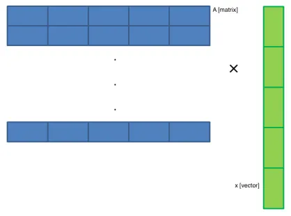
In an OpenCL environment, libraries exist which perform linear algebra tasks, including

matrix-vector multiplication, in an OpenCL environment. A custom algorithm is presented

alongside this solution for reasons discussed in a later section. The custom algorithm

per-forms a two-phase reduction for each dot product; first, N_P multiplications and N_P additions

are performed on each ofp=P processing elements. Following this, additive reduction is

performed inlog2(P)stages. Figures 4.1, 4.2 and 4.3 illustrate this basic approach.

The value ofP is chosen to satisfy two criteria: P = 2K _{for some integer}_K_{, and}_P

is close to the number of processing elements available. The first criterion ensures that the

second phase (binary phase) of the reduction is possible, while the second one ensures that

the first phase of the reduction executes as quickly as possible by exploiting the maximum

level of parallelism. For many available platforms, both criteria can be satisfied because

the total number of processing elements is a power of 2, or the preferred number of

simul-taneous threads is a power of 2.

Because heterogeneous systems often have a large communication penalty, and the

matrix-vector multiplication requires using all of the training data available to the SVM, it

is worth considering measures to mitigate this cost. For this reason, a cache is maintained

which keepsX data stored on the device where the calculation is being performed.

LIB-SVM makes use of a shrinking working set and frequent reordering, so each swap in the

main algorithm is mirrored on the OpenCL device used to perform KM calculation in order

to keep the cache valid. This trades the communication cost for the training vectors with

the cost of executing the swapping kernel on a regular basis, which in practice is found to

(42)

Figure 4.1: Illustration of Matrix-Vector Multiplication

[image:42.612.205.414.106.261.2]

Figure 4.2: Parallelization of Matrix-Vector Multiplication. Colors indicate division of labor amongst work groups

(43)

This kernel calculation is used both in the training and classification phases of the SVM,

and thus is central to the overall, accelerated system. However, it makes up a much larger

percentage of the training phase than it does the classification phase, and so, given that total

acceleration will hinge on this operation, we expect to see that training is accelerated to a

greater degree than classification, as per Amdahl’s law.

Custom Work

One of the many benefits of OpenCL is its platform independence and flexibility;

through the use of its powerful APIs and supporting abstraction layers, OpenCL

applica-tions can be made extremely portable while still exploiting the benefits of high performance

devices available in a hetergeneous system. Furthermore, third party library support offers

a range of functionality that is easy to use and thoroughly debugged and often doesn’t

re-quire the user to write any OpenCL kernels. This can drastically reduce development time

for large applications.

However, this flexibility could come with a performance penalty. Specifically, third

party libraries often have to remain very general, offering a broad range of capabilities; this

typically means that the capabilities offered are not highly optimized for a specific

prob-lem and a performance gain could be achieved through a fully custom impprob-lementation. An

opportunity is presented to trade development time for improved performance.

In this work, both approaches are considered. In one approach, a custom set of OpenCL

kernels are written and tuned to achieve the maximum performance for the specific problem

being approached. This involves a greater effort, but it is expected to provide a worthwhile

improvement in performance. In the second approach, the OpenCL AMD BLAS library is

used to perform the calculations used in the SMO algorithm and a minimal amount of

cus-tom OpenCL code is used. In this way, one can analyze the tradeoff between development

(44)

4.1.2 Training

Solving Single Step

The main training algorithm, SMO, is an iterative approach and that the central

com-putation in each iteration is solving for two values of α with respect to each other. This

solution requires calculations of K(~xi,~xi), K(~xj,~xj) andK(~xi,~xj), here denoted Qii,

Q_jj andQ_ij in reference to theQmatrix. However, because of the values used in the next

step, the work presented calculates two entire columns of theQmatrix instead of just three

values, here denotedQ_iandQ_j.

Due to this requirement, the basic function of this implementation is a modified kernel

function which performsK(X,~xi). While it is the case that a single OpenCL kernel could

be used to calculate X~xT_i , and this kernel could be shared by all of the kernel functions

followed by a smaller OpenCL kernel which calculates h(·), this approach is not taken.

Each kernel function is implemented by a single OpenCL kernel which performsX~xT_i and

thenh(·)to avoid the overhead of executing two kernels.

During calculation of a single column of the kernel matrix, the steps shown in

Algo-rithm 1 are performed on the host device. The corresponding CU device code is shown by

Algorithm 2; this is the same operation illustrated in the previous figures.

Once the kernel matrix column is calculated, it is cached on the host side. This is a

significant optimization, since each iteration of the training algorithm uses the calculation

multiple times. The last step in solving a single pair of values is a calculation which is left

to the host, since the host processor is best suited to it, as it involves a small number of

expensive operations and some amount of flow control.

Objective Function Updating

The objective function which tracks the gradient of the function being optimized is used

for the stopping conditions

(45)

Algorithm 1Q Matrix Column Calculation

ifX is cached on the devicethen

store its buffer in X BUFFER

else

create OpenCL buffer X BUFFER

enqueue command to write X to X BUFFER

end if

ifx i is cached on the devicethen

store its buffer in X I BUFFER

else

create OpenCL buffer X I BUFFER

enqueue command to write x i to X I BUFFER

end if

wait for all write commands to finish

enqueue command to run kernel function kernel on device, operating on X BUFFER and X I BUFFER

wait for kernel function to finish

enqueue command to read Q i from device to host wait for read command to finish

Algorithm 2CU Device Code For Calculating Kernel Matrix Column

1: store row number in R

2: store local work group element number in T

3: store number of columns in COLS

4: store size of local work group in WG

5: sum := 0.0

6: startIndex := T

7: whilestartIndex < COLSdo

8: sum := sum + A[ R * COLS + startIndex ] * x[ startIndex ]

9: startIndex := startIndex + WG

10: end while

11: scratch[ T ] := sum

12: local work group barrier

13: offset := WG / 2

14: while of f set >0 do

15: ifT < of f setthen

16: scratch[ T ] := scratch[ T ] + scratch[ T + offset ]

17: end if

18: local work group barrier

19: offset := offset / 2

20: end while

21: if T = 0 then

22: y[ R ] = h( scratch[ 0 ] )

(46)

This function is updated at each iteration.

~

gr+1 =~gr+ (α~r_i+1−α~r_i)y~_iQ_i+ (α~r_j+1−α~j)y~jQj (4.10)

The value of Qi, Qj is cached prior to this operation, but the update is still a vector

addition operation on a vector of length M with a complexity of O(M). It is worth

not-ing that each element of gr+1 requires two double-precision floating point multiplications

and three double-precision floating point additions (the difference inαvalues need only be

computed once), so itsO(·)representation belies its true computational cost.

This is another point where both a custom implementation and a solution based on a

prefabricated library are presented. The custom implementation is extremely

straightfor-ward — it simply performs the five operations in parallel for every index of g. However,

this presents an issue: the value of the function is required at certain points in the sequential

portion of LIBSVM, so the value needs to stay synchronized between the device where it

is computed and the primary CPU. For this reason, two configurations for this algorithm

are considered.

First, the calculation is performed on the available GPU, for varying values ofM, then

the same algorithm is moved to a parallel view of the CPU, using OpenCL to generate

par-allel extension instructions in a platform agnostic manner, and again observed for varying

values ofM. Both of these are compared in terms of performance with a closely measured

sequential version (found in the unaltered LIBSVM code).

Working Set Selection

The working set is selected as follows

i∈arg max

t {−~yt∇f(α~ r

)t|t∈Iup(α~r)}

j ∈arg min t

−b

2 ij

a∗_ij|t ∈Idown(α~ r

),−~y_t∇f(α~r)t <−~yi∇f(α~ r

(47)

Select i Calculate Qi Select j |f’(i) - f’(j)| ≥ ϵ

NO Reconstruct Gradient

Select i

Calculate Qi

Select j

|f’(i) - f’(j)| ≥ ϵ NO

Stop YES

Calculate Q_j

Optimize

αi, αj

Update f

[image:47.612.118.504.92.297.2]

YES

Figure 4.4: LIBSVM Algorithm Flowchart

whereiis selected first, which amounts to iterating over the objective value searching for

a maximum under a few prerequisite conditions. This is anO(M)operation, and can be

reduced through a parallel reduction toOM log2(M)

p

. Selection ofj follows sequentially

after the selection ofi, because it depends oni, and sees the same speed up fromO(M)to

OM log2(M) p

.

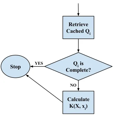
For reference, 4.4 is reproduce here; in addition, the calculation of a row of the Kernel

Matrix is expanded into 4.5. This is the phase of the algorithm that has been most

signifi-cantly altered in order to accelerate LIBSVM; 4.6 shows a high level view of the alteration

made. The scalar kernel function calculation is omitted due to its simplicity, however, the

parallel kernel function computation algorithm is shown in 4.7.

4.1.3 Classification

The classification phase of the SVM system is a much simpler algorithm than the

(48)

Retrieve Cached Qi

Q_i is complete? Stop YES

Calculate K( x_i, x_j )

[image:48.612.199.410.112.362.2]

Append to Q_i NO

Figure 4.5: Kernel Matrix Row Calculation Flowchart

Retrieve Cached Q_i

Q_i is Complete? Stop

Calculate K(X, x

i) YES

NO

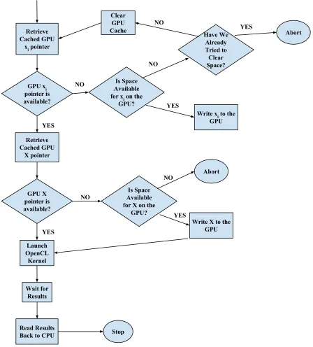
[image:48.612.210.396.456.646.2]

(49)

Retrieve Cached GPU

x_i pointer

GPU x_i pointer is available?

Is Space Available for x_i on the

GPU? Have We Already Tried to Clear Space? Abort Clear GPU Cache

Write xi to the GPU Retrieve Cached GPU X pointer GPU X pointer is available? Is Space Available for X on the

GPU?

Write X to the GPU Launch OpenCL Kernel Wait for Results Read Results

Back to CPU Stop

[image:49.612.100.548.133.629.2]

NO YES YES NO NO YES NO Abort NO YES YES

(50)

and the vectors to be classified, and evaluates the decision function.

D(~x) =X

i ~

αiK(x~i,~x) +b

Here, x~i are the support vectors andx is the vector being classified. For the sake of

efficiency and code reuse, this function’s representation is slightly modified.

D(~x) =αK~ (X,~x) +b

K(X,~x) =



   

K(x~0,~x)

K(~x1,~x)

...     

In this form, the parallel kernel function code previously described can be reused for

this phase. Following this, a new OpenCL kernel is used to perform the inner product ofα~

andK(X,~x)using parallel reduction as described previously.

4.2

Comparisons

4.2.1 Overview

In this work, two comparisons are made between the presented version of LIBSVM

and the reference version. First, the performance is compared in terms of execution time.

This is important as speedup is the main advantage OpenCL implementation claims to

offer over the existing library. Secondly, the difference in output between the two versions

is measured, because a performance improvment at the cost of accuracy is unacceptable in

many cases. We refer to the error as the amount that the HSA output differs from the serial

(51)

4.2.2 Timing

High performance and serial implementations are both timed using native, OS

sup-ported timing tools such as the time.h library for UNIX-based systems and the performance

counter under Windows. Processing time, i.e., the time taken to execute a kernel, is

consid-ered separately from communication time and setup time for OpenCL implementations to

provide a thorough, fair comparison; this lends insight into which situations are well suited

to the methods presented here.

The contributed SVM algorithm is compared to the existing LIBSVM executable for

training and classification. The operation is timed at two levels; first, the entire time taken

to execute the standalone binaries are measured using the time module inside Python. This

is important, because the end user of the system will be primarily concerned with this time

and the resultant speedup. Additionally, performance is measured and observed for each

stage of the algorithm individually, including OpenCL kernel execution time,

communica-tion time and compilacommunica-tion time. This provides a more thorough understanding of the nature

and causes of any resultant speedup and will highlight the benefits and drawbacks of the

OpenCL system.

4.2.3 Error

Two comparisons are made between the output of the high-performance SVM

imple-mentation and the existing LIBSVM impleimple-mentation. First, the SVM model file produced

by the two executables will be compared; this is the most important comparison, because

the two files being identical ensures that the new implementation has made the same

deci-sions as the reference implementation, as the same supporting vectors were selected with

the same final objective function.

This check is important because, while OpenCL provides guarantees about its error for

single-precision floating point operations, LIBSVM requires the use of double-precision

(52)

the availability, implementation or accuracy of double-precision floating point operations,

therefore some calculations may present an error with respect to the reference calculations

due to floating point inconsistencies, but this error may be within tolerance for certain

datasets and applications. In the next chapter, we describe the specific problems to which

(53)

Chapter 5

Results

5.1

Performance

Hardware

All tests for this section are performed using the same desktop computer work station.

It contains an Intel i5 quad core processor operating at 3 GHz used to run the reference

implementation of LIBSVM; LIBSVM is neither written, nor adapted in this set of tests,

to run on

High Performance Implementation of Support Vector Machines Using OpenCL