Bipartite guidance, navigation and control architecture for autonomous aerial inspections under safety constraints

(will be inserted by the editor)

Bipartite guidance, navigation and control

architecture for autonomous aerial inspections under

safety constraints

Giuliano Punzo _· Charles Macleod _· Kristaps Baumanis _· Rahul Summan _· Gordon Dobie · Gareth Pierce · Malcolm Macdonald

Received: date / Accepted: date

Abstract In this work the autonomous flight of a drone for inspection of sensitive environments is considered. Continuous monitoring, the possibility of override and the minimisation of the on-board computational load are prioritized. The drone is programmed with a Lyapunov vector guidance and nonlinear control to fly a trajectory passed, leg after leg, by a remote ground station. GPS is the main navigation tool used. Computational duties are split between the ground station and the drone’s on board computer, with the latter dealing with the most time critical tasks. This bipartite autonomous system marries recent advancements in autonomous flight with the need for safe and reliable robotic systems to be used for tasks such as inspection or structural health monitoring in industrial environ-ments. A test case and inspection data from a test over flat lead roof structure are presented.

Keywords UAV · Bipartite architecture· Lyapunov vector field · Industrial applications·Autonomous Aerial Inspection·Roofs

1 Introduction

Inspection, surveillance and health monitoring are increasingly becoming popular application areas for unmanned aerial vehicles (UAVs or drones) [1–5]. Inspecting industrial assets for health monitoring is a necessary activity. Elements such as high stacks or surface poor conditions of the dedicated inspection paths due to continuous weather exposure make this a risky activity for human operators [6]. In the inspection of elevated areas, such as roofs and chimneys, the safety com-ponent has substantial cost implications as well [7]. Automation put in place in this sector often aims to avoid the exposure of human operators to such hazards. This has motivated the development of autonomous robotic systems suitable for industrial inspections [8–11]. Previous works addressing this problem, such as [6,

G. Punzo

9, 1, 2, 4, 8, 12]. concentrated their attention on drones. Despite already used for inspection tasks, mainly as remotely piloted vehicles, guidance, navigation and control (GNC) of drones is the object of continuous industrial research. Tech-niques depend on the performance required: long range UAVs, usually with fixed wing, perform their missions kilometres away from the base: position accuracy and obstacle avoidance are secondary when compared to turn planning [13] or the tra-jectory generation for these vehicles [14]. Conversely, rotating wing devices, have shorter range but superior low speed performance, with the ability of hovering on the spot and manoeuvring in small spaces. These devices are hence ideal for tasks such as surveillance of small regions, structural health monitoring and flying in confined environments or indoors. For both fixed and rotating wing vehicles, a very popular approach relies on the to-point navigation with the path defined by waypoints. Robust implementations of this technique have now reached the mar-ket: popular examples are the Pixhawk electronic kits [15] or the ASCTEC drones [16], one of which has been used for this work. However these are characterised by aiming to the waypoint rather than flying the leg between pairs of waypoints at desired speed or attitude.

While the interest of the industrial world and the case for continuous research are clear, applications of drones in industrial environments are still heavily limited by safety constraints. These are in place to protect high value assets, (e.g wind turbines) for which autonomous systems are seen as a risk. The presence of a human supervisor, able to override the system, is a non-optional feature. Some-times it is possible to observe a clear contrast between supporters of autonomous technology, firmly convinced of their safety, and their sceptic opponents. Together with increasing the technology readiness level (TRL) of autonomous technologies, it is important to have viable solutions to perform autonomous inspections that satisfy the safety objections and any scepticism. There is then a scope for tech-nologies whose value and safety can be agreed by both sides in the dispute [17–19].

being helped in this by the architecture of the controller that requires no changes to the software on the drone. Our analysis focusses on the control architecture rather than the drone performance as inspection system. We thereby use a commercially available platform without adding any ad-hoc sensors (e.g. proximity sensors) or computational capabilities. In the second part of this paper we report about a raster scan performed to survey a building with lead roof and rectangular shape, as a test case. Using image mosaic and processing we obtain good quality data using commercially available visual sensors designed for general purposes. The results obtained indicate the suitability of the GNC architecture for extension to sensors beyond visual ones, such as laser/lidars or acoustic sensors.

2 Control System Architecture

The control of the drone is composed of two separate software parts: the on-board and the ground segment. The on-on-board segment features the non-linear guidance and the control making the drone approach a straight line trajectory and follow it at a desired speed. This part is coded in Matlab, compiled in C and downloaded to the hardware [25]. The ground segment is also coded in Matlab but is not compiled nor downloaded. It runs in real time and interfaces with the on-board segment by updating the waypoints defining the legs to navigate and logging the telemetry. Both the transmitted and received streams are broadcast using a universal asynchronous receiver/transmitter (UART) X-bee devices with a IEEE802.15.4 protocol. Figure 1 shows the task division and the communication between the ground and the on-board segment.

Fig. 1:General Scheme of the software setup.

2.1 Ground segment

as dashboard.

In receiving, it decodes and displays the UART data. These include a subset of the readings taken by the on-board instruments. This subset is customizable. There are 50 channels in total, the first 10 channels are refreshed at a maximum of 100Hz, while the others are cycled in groups of 10.

In transmitting, the ground segment passes the waypoints, reading a pre-loaded list of latitude and longitude values. It takes them in pairs, so to define the raster scan legs to follow. To produce the list, the coordinates of the pattern’s centre and its size (i.e. the radius of the trajectory envelope or the leg’s length) are to be manually inserted. For each pair only the destination is passed together with the sine and cosine of the heading angle from the North. These components remain constant for the time the drone flies the leg, hence are calculated offline when ini-tialising the ground station. This allows saving on-board computational resources. There are 10 UART channels available for transmission and 4 of them are taken by the leg information. The other 6 are used to tune the proportional and derivative gains of the controller, to send an open-loop command for the thrust and a code that defines the cycling frequency of the last 40 UART receiving channels.

2.2 On-board segment

The on-board segment implements the core of the guidance, navigation and con-trol algorithms. This is coded in Simulink, then compiled in C and flashed to the drone on-board computer. This piece of software receives the data from the drone navigation instruments. These include the inertial sensors, the GNSS, the magne-tometer and the pressure sensor for the height. The on board segment implements a line-following algorithm as any trajectory is segmented into a sequence of parallel straight lines, linking waypoints. For this reason, the on-board segment just has to follow the straight line passed, time after time, by the ground segment. This is achieved by superimposing 2 desired velocity vector fields, the ”across” field and the ”along” field. Further details about this are given in Section 3.1.

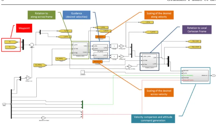
The line-following algorithm is part of a more complex architecture described in Figure 2. First the navigation is implemented with the position obtained through the GPS. This is translated into a local, metric grid, reducing over/underflow re-lated problems, and aligned onto the trajectory leg to follow. Further details about the reference frames and the processing of the navigation are reported in Section 2.3.

Fig. 2:Flow diagram of the functional blocks composing the on-board software segment. Lat-Long refers to the coordinates provided by the GNSS, these are transformed to a planar, local reference (To Gird(East-North), To Local Grid) and aligned to the trajectory leg to follow (To along-across grid). See Figure 4 for the details of these reference frames. The desired velocity is then computed as a vector in the along-across frame, scaled (tuning) and translated back to the North-East frame for comparison with the actual velocity from the GPS. This is finally transformed to body axes and passed to a controller to command roll and pitch of the drone. The centre of the figure shows the ideal approach and following of a trajectory leg and the desired velocity vector field for a leg parallel to the vertical axis.

electric motors. The code that transform commanded angles into motors voltage is part of the ASCTEC proprietary software, hence not editable.

2.3 Reference frames

Six different reference frames have been considered in developing the drone control architecture. These are:

– Latitude-Longitude (LL);

– Local Latitude Longitude (LLL);

– Local Cartesian Frame (LCF);

– Local North-East Frame (LNEF);

– Along-Across Frame (AAF);

– Body Reference Frame (BRF).

Fig. 3:Snapshot of the Simulink implementation of the GNC algorithm.

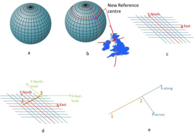
system to work effectively the origin should not be set more than 5 degrees in Lat-itude and LongLat-itude away from the mission area. The offset of the reference frame bounds the size of data that have to be transmitted to the drone for navigation purposes. This is necessary given the limited number and type of transmission channels available. The LLL is computed on-board by subtracting the offset from actual GPS reading.

The LCF is obtained by passing from angular coordinates in the LLL to linear, metric ones. The grid, in this case, is centred on the zero of the LLL. LLL co-ordinates are mapped to an ellipsoid whose radius is function of the latitude (as obtained in the LL), according to Equation (1)

R=R(φ) =

s

(a2_cosφ)2_{+ (b}2_sinφ)2

(acosφ)2_{+ (bsinφ)}2 (1)

where, φis the latitude,a is the Earth equatorial radius ( 6,378.1370 km) andb is the polar radius (6,356.7523 km). LCF coordinates are obtained as

XLCF =R(φ)∆ψ

YLCF =R(φ)∆φ (2)

where, ∆φ and ∆ψ are, respectively, the Latitude and Longitude as mapped in the LLL.

For each waypoint the drone aims to, the LCF is shifted taking the waypoint as origin. This produces the LNEF, which changes after the waypoint is acquired, moving to the following waypoint.

to the right of the track. If the leg is oriented exactly from South to North, LNEF and AAF coincide. This five frames are sketched in Figure 4.

Finally, the BRF is referred to the vehicle body axis. This is centred in the centre of mass of the drone, assumed to coincide with its geometric centre for simplicity. According to the popular aeronautics convention, the x-axis is pointing the drone front, the y-axis points to the right of the vehicle and the z-axis points downwards to complete the right-handed frame. This is sketched in Figure 5. The BRF is of fundamental importance for control as attitude is defined as its rotation with respect to a fixed one. The pitch corresponds to the vehicle rotation around the BRF y-axis, the roll around the x-axis and yaw around the z-axis. They are positive or negative if the angular velocity vector has the same (positive) orientation of the axis or the opposite (negative).

Fig. 4: Reference frames used in the guidance, navigation and control algorithm. a. The

Fig. 5: Body reference frame used. This is in accordance with the aeronautical convention. Images adapted from [25]

3 Guidance, Navigation and Control

3.1 Guidance

The guidance is provided as a 2D velocity field. This is in line with the strategy adopted in [26], where a fixed wing autonomous vehicle is considered. Every point in the horizontal plane containing a desired straight path can be identified by its distance with sign from the path in the orthogonal direction (x-acrossorxac) and

its distance from the final point of the path in the direction parallel to the path (x-along or xal). This corresponds to the coordinates being defined in the AAF

(see Section 2.3). The velocity field provides, for each (xal,xac), onealongand one across velocity components, (valandvac respectively), whose vector sum returns

the desired velocity for the drone to track at every position. The across velocity is everywhere orthogonal to the line to follow and produces the convergence to the desired trajectory. Its magnitude increases with the distance from the line, being null on the line. The along velocity is everywhere parallel to the line. Its magnitude increases with the distance to the final waypoint defining the line, where its magnitude vanishes. By tracking the resultant velocity field the drone is driven onto the desired path through a smooth trajectory. To make the drone first approach and then follow the path,vac must dominatevalat large distances,

while, when on the path, val must dominate vac. As this work mainly looks at

inspection paths, we defined the along component to be approximately constant on the path, and to reduce to zero when approaching the end of it. Equations (3) and (4) produce this behaviour.

vac= xac

cac+kac|xac|

(3)

val= xal

cal+kal|xal|

S(xac) (4)

where, | · | indicates the absolute value and S(xac) = 1/(Kx2ac+C) regulates

were chosen simulating the dynamics and refined through a trial-error process and are: cac = 1,kac = 1, cal = 1, kal = 1, C = 0.5 andK = 2. The functions in

Equations (3), (4) andS(xac) are plotted in Figure 6.a, while the resulting vector

field is plotted in Figure 6.b for a straight trajectory with heading 45o _{from the}

North. Note that the along and across track velocities (Equations (3) and (4)) can be further scaled to meet the speed requirements dictated by the task to be performed, as previously discussed. This can be done operating on the ground segment without requiring any change in the guidance algorithm on the drone.

-10 -5 0 5 10

x-across or x-along [m] -1 -0.8 -0.6 -0.4 -0.2 0 0.2 0.4 0.6 0.8 1

Nondimensional Desired Velocities

Desired velocity along and across the track Scaling of the along velocity with x-across

-10 -5 0 5 10

X-East [m] -10 -8 -6 -4 -2 0 2 4 6 8 10 Y-North [m] (a) (b)

Fig. 6: a. Along and across the track desired velocities. The function is the same but it can be scaled differently for along and across directions. The magnitude of the along component is further scaled as a function of its distance from the desired trajectory. b. Vector field resulting from the guidance law for a straight trajectory heading 45o_.

3.2 Navigation

A GPS receiver is available and already integrated with the hardware on the ASCTEC Firefly. Typical GPS horizontal accuracy with high quality receivers is down to 3.5 metres [27]. The velocity is obtained through the GPS as well, while the attitude is obtained through data from the inertial sensors and the compass. Finally, the altitude is obtained through a pressure sensor, already part of the ASCTEC drone which we found sensitive to wind, and fouls the proprietary height control loop, producing sudden drops and rises. This prevents the drone from keeping a constant height and, in turn, limits the vertical closeness achievable to any inspection target.

3.3 Control

exclusion of this component from the on-board software. The option of calculating the integral part on the ground segment was considered too, but this was discarded for the possible lags in communication between the ground and the aerial segments. The design was finalised with a proportional-derivative (PD) controller. Because of the non-perfect central symmetry of the drone, 2 separate sets of gains for pitch and roll are used. These are: pitch proportional gain = -0.25; pitch derivative gain = -0.005; roll proportional gain = 0.26; roll derivative gain = 0.02.

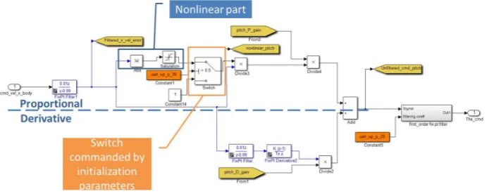
3.3.1 Close-range nonlinearities and Filtering

A non-linear transition is implemented to provide zero derivative between positive and negative commands. This reduces the oscillations due to noise in the navigation and is visible in the Simulink scheme of Figure 7. A cascade of first order filters is

Fig. 7:PD controller for the pitch featuring the nonlinear part. This can be set at initialisation through setting the switch state.

used, providing a low pass filtering effect through a moving average mechanism. In this, the signal (GPS data) is filtered through the recursive scheme yn = a∗

yn−1+ (1−a)un, that is, the signaly, at stepnis obtained as weighted average

3.4 Algorithm tuning

Both the guidance and the control algorithms were tested through a Simulink quad-copter model developed at Drexel University [28]. The simulator was edited and adapted to the ASCTEC Firelfly after a series of characterisation flights. Through the simulator, all the constants present in the guidance and control equations were tuned proceeding by a trial-error process. Moreover, as the model is coded in Simulink, the guidance and control algorithm tested could be compiled and down-loaded to the drone with minimal editing due to the limitations in computational power of the on-board processor.

Table 3.4 summarises the reference frames involved in the various tasks of the autonomous flight and the requirements for these to be carried out through fast or slow dynamics.

Table 1: Summary table of autonomous flight tasks. The Navigation has a fast acquisition

dynamics in the aerial segment for control purposes but the speed of processing for guidance purposes is not as a stringent requirement, so it can be passed onto the ground segment. In the same fashion the inspection data acquisition needs a fast dynamics but its logging can be delayed.

AUTONOMOUS FLIGHT TASK Frame Segment Dynamics

Guidance AAF Ground Slow

Navigation LL Aerial Fast

All Ground Slow

Control BRF Aerial Fast

Inspection - Aerial Fast

Logging - Ground Slow

4 Results

Control architecture performance were evaluated in open, agricultural land. Tests were carried out in a variety of weather conditions so to evaluate the system in both still air and windy conditions.

4.1 Still air performance

expectations. Finally the position error across the track is shown in Figure 8.c The across distance oscillates mainly because of the position measurement errors. Table 2 summarizes the performance for speed and position errors. A reduced set of measurements, that do not consider the transient phase as waypoints change, consisting of all the data-points within 1 m error, are shown as well in Table 2 and Figure 8.c.

4.2 Performance is side wind conditions

In this test-case two passages are performed for the same scanning pattern. The circular region for the scanner path has 8 m radius with waypoints considered achieved when within 1.5 m distance. This test was performed with lateral wind between 6 and 8.5 m/s (13.4 and 19 mph respectively). Table 3 summarizes the performance in side wind conditions. Also in this case a reduced set of errors under 2 m is considered to exclude the transitory effect of waypoint switching.

-10 0 10 20

X-East [m] -15 -10 -5 0 5 10 Y-North [m]

40 60 80 100 120 140

time [s] -2

0 2

Velocity [m/s]

V along and across

Velocity along the track Velocity across the track

40 60 80 100 120 140

time [s] -50

0 50

Position [m]

X along and across

Position along the track Position across the track

(a) (b)

40 60 80 100 120 140

time [s] -10 -8 -6 -4 -2 0 2

Across-track Position Error [m]

1 m error or more Less than 1 m error

(c)

Table 2:Summary table of positioning and velocity performance in still air conditions. Mean Standard Deviation Across-track position error -1.519 m 2.128 m Across-track position error (<1mdata points) -0.218 m 0.391 m X velocity error (BRF) -0.183 m/s 0.882 m/s Y velocity error (BRF) 0.148 m/s 0.939 m/s

Test duration: 76.4 s

Table 3:Summary table of positioning and velocity performance in windy conditions.

Test Mean Standard Deviation Across-track position error Test 1 1.472 m 0.993 m

Test 2 1.910 m 1.183 m Across-track position error (<2mdata points) Test 1 1.196 m 0.723 m Test 2 1.322 m 0.726 m X velocity error (BRF) Test 1 0.991 m/s 0.631 m/s

Test 2 -0.232 m/s 0.567 m/s Y velocity error (BRF) Test 1 -0.547 m/s 0.568 m/s Test 2 -1.135 m/s 0.619 m/s Test duration: 44.7 s (test 1), 55.7 s (test 2)

5 Autonomous Inspection Test Case

A complete testcase, featuring flying raster scan trajectories and collecting images at the same time was carried out on 30th _{September 2015 on a private property}

featuring a lead roof. As different from the test in agricultural land, for this test case, as in many real industrial inspections, the centre of the scan was not reachable by a physical person, hence it was estimated as 11 metres South from a surveyed point. Because of the geometry, the scan was designed on a rectangular domain with sides 14 m and 15 m through adapting the trajectory generation algorithm running on the ground segment initialisation. Once again, the architecture made this operation straightforward. The raster scan legs were placed 2m apart. The wind speed during the test remained below 2 m/s. Figure 9 shows the configuration of the test setting.

5.1 Tracking and performance measurement

The flight path was tracked externally using a Leica AT901-B single point laser tracker. This is a metrology system with an accuracy of 0.2µm+15µm/m. A prism reflector with an acceptance angle of ±50◦ _{was attached to the underside of the} UAV such that line of sight could be maintained during flight. The laser recorded the (X, Y, Z) position of this reflector which served as the ground truth trajectory for each flight.

5.2 Image sampling and reconstruction

Fig. 9:Sketch of the test setup. The trajectory to follow is reported in red while the roof lines are in blue. The shaded area at the left of the picture represents a chimney.

barrel distortion resulting from the lens was removed using the GoPro proprietary software. A subset of 5 frames were then extracted from the video to produce an image sequence covering the inspected area shown in Figure 11a and b. The Scale Invariant Feature Transfrom (SIFT) was used to extract image features from these images [29, 30]. Specifically, the SIFT features are used to estimate the homography matrix which relates the images. Note this transformation has been applied with the assumption that the observed surface is planar or very close to planar. The orthographic view of the roof, obtained through the homography transform of the composite image, is shown in Figure 11.c

5.3 Flight path accuracy

The 3D positions from the laser tracker were registered, together with the 2D (X, Y) positions from the GPS and the desired path to produce the plots referring to two separate runs in Figures 10.a and 10.b, these are shown in theXY plane. It can be seen that the GPS and laser paths have a largely similar shape with the GPS path being heavily quantized. The error between the GPS and laser paths were computed by comparing each GPS data point with the closest point recorded by the laser and with the desired paths. This corresponds to

ex= min xl

X−xl

ey = min xl

where,xl, ylare the laser data whileX, Y are the GPS data. The errors expressed

in terms ofX andY components are tabulated for runs 1 and 2 in Tables 4 and 5 respectively.

-5 0 5 10 15

X-Axis [m]

-8 -6 -4 -2 0 2 4 6 8 10

Y-Axis [m]

GPS data Leica data Desired

-5 0 5 10 15

X-Axis [m]

-8 -6 -4 -2 0 2 4 6 8 10

Y-Axis [m]

GPS data Leica data Desired

(a) (b)

Fig. 10:Leica Positional Data. (a) first run; (b) second run

Path Comparison Minimum (m) Average (m) Maximum (m) Std Dev (m)

Leica vs GPS (X-axis) 0.0001 0.2568 3.629 0.583

Leica vs GPS (Y-axis) 0.0002 0.0092 0.6128 0.0426

Desired vs GPS (X-axis) 0.0715 0.1451 0.3667 0.0734 Desired vs GPS (Y-axis) 0.0125 0.6886 4.1563 1.2204 Desired vs Leica (X-axis) 0.0011 0.5575 3.8509 1.1993 Desired vs Leica (Y-axis) 0.0002 0.7209 4.4445 1.3751

Table 4:Axis errors Run 1

Path Comparison Minimum (m) Average (m) Maximum (m) Std Dev (m)

Leica vs GPS (X-axis) 0.0002 0.3503 6.2652 0.751

Leica vs GPS (Y-axis) 0.0003 0.0066 0.6932 0.0376

Desired vs GPS (X-axis) 0.0715 0.2359 1.4673 0.3616 Desired vs GPS (Y-axis) 0.0024 0.6001 3.5456 1.0259 Desired vs Leica (X-axis) 0.0001 0.6686 4.2456 1.3441 Desired vs Leica (Y-axis) 0.0001 0.6837 4.2388 1.3029

Table 5:Axis errors Run 2

6 Discussion

(a) (b) (c)

Fig. 11:Aerial Images: (a) Individual images used in mosaic; (b) Composite image constructed from the 5 images; (c) Levelled out composite image

the advantages obtainable through autonomy. On one side the research commu-nity pushes towards prototyping new control laws; on the other side there is the industrial community, considering in their best interests the reliability issues when approaching new tools and procedures. Here we presented a solution that could be adapted and agreed by both sides, that is splitting the control algorithms in 2 parts, so to diminish the risk of malfunctioning on the inspector side.

The manual override, so far considered the natural back-up to any unforeseen behaviour of the autonomous inspecting vehicle, is still present, but becomes the third safety element of the command chain. First there is the drone, that enter station-keeping mode when not in contact with the ground station; then there is the ground-station, directly under the supervision of a human operator. Finally there is the remote pilot, who can regain control of the inspecting vehicle at any time. Devolving part of the tasks to the ground stations reduces the computational load on-board the vehicle and, consequently, the associated risk. This is one step beyond with respect to relying on manual override alone, which seems to be the most popular solution currently used.

posi-tion error. We did not investigate these and concentrated instead on proving the concept through collecting inspection data. Nonetheless the errors are within the accuracy of the current GPS technology.

A more compelling issue is the suitability of GPS in environments where the pos-sibility of signal loss exists due to loss of line of sight, or scattering. Relying on GPS is not sufficient for navigation - indeed under CAA rules it is not sufficient to use GPS alone. At least two techniques for position determination must be used when the remote pilot has obstructed line of sight. GPS only is accepted in case of a remote pilot having continuous line of sight. In this regard, although our work addresses significant implementation issues, it does not present a system ready to be deployed on the autonomous inspection market. Instead it paves the way for better equipped vehicles to be accepted by an always greater user community by devolving part of their function to the ground station, through which continuous direct control is possible.

The GPS horizontal accuracy of few metres may be coarse for some observation tasks, especially if a stable, close looking base for asset assessment is required. This problem, however is secondary with respect to the altitude keeping issue. Proximity to an inspection target was limited vertically rather than horizontally due to sudden changes of pressure. The aerial platform used for this case study measures the height based on a pressure sensor and accelerometers. Oscillations in the order of metres were observable because of noise in these sensor measurements and wind changing the local pressure reading. For a downward looking sensor, a far field was the only viable option and the positioning in the horizontal plane in this scenario loses importance. While conceiving that GPS alone may not be enough for some industrial inspection, we think that proximity sensors should be the first option to enable closer inspections. The presence of a ground station naturally offers scope for differential navigation. This is at the moment the most promising direction to improve the system performance, at least for what concerns outdoor inspections.

Improvements are possible also in the Lyapunov vector method used, as previously discussed. We concentrated on constant inspection speed, height and heading, relying for the last two on the drone built-in sensor suite and dealing this way with a two-dimensional field. 4D vector fields including the active control of height and heading, are also possible, as it is possible to make the scanning speed change arbitrarily while flying each leg. All this is not implemented here as beyond the scope of the work.

The Go-Pro camera is not a tool designed for remote inspection. The problems arising from lens induced distortions and the field of view have hence been tackled through image post-processing, that proved a viable solution to compensate, in part, for poor quality visual inspection data.

7 Conclusions

This work proposed a control architecture and a guidance law suitable to perform autonomous aerial inspections in areas where safety constraints are present. Host-ing some of the computational duties on a remote ground station decreases the risk of saturating the on-board computer while allowing flexibility in the design of the scanning trajectory. The use of a Lyapunov vector guidance, often applied to fixed wing vehicles, revealed viable, yet improvable, for rotating wing UAV operating at slow speed. The position accuracy obtained is well within the limits of the cur-rent satellite navigation technology, yet improvements are possible through a more refined navigation sensor suite or different navigation means, such as differential GPS, radio frequency identification and object recognition. Such improvements are also likely to enable better altitude measurements, hence control, which was deliberately overlooked in the present study but which we acknowledge being a fundamental issue in driving the technology into application effectively.

In the contrast between the need for advances in automation and the scepticism on the safety raised by current autonomous technology, we indicated a way to a potential win-win compromise.

References

1. P. Quater, F. Grimaccia, S. Leva, M. Mussetta, M. Aghaei, Photovoltaics, IEEE Journal of4(4), 1107 (2014)

2. M. Rossi, D. Brunelli, Instrumentation and Measurement, IEEE Transactions onPP(99), 1 (2016)

3. A. Kolling, A. Kleiner, P. Rudol, in Intelligent Robots and Systems (IROS), 2013 IEEE/RSJ International Conference on(2013), pp. 6013–6018

4. J. Villasenor, Proceedings of the IEEE102(3), 235 (2014)

5. J. Nikolic, M. Burri, J. Rehder, S. Leutenegger, C. Huerzeler, R. Siegwart, IEEE Aerospace Conference Proceedings (2013). DOI 10.1109/AERO.2013.6496959

6. A. Ortiz, F. Bonnin, A. Gibbins, P. Apostolopoulou, M. Eich, F. Spadoni, M. Caccia, L. Drikos, Proceedings of the 15th IEEE International Conference on Emerging Tech-nologies and Factory Automation, ETFA 2010 pp. 1–6 (2010). DOI 10.1109/ETFA.2010. 5641246

7. G. Bartelds, Journal of Intelligent Material Systems and Structures9(11), 906 (1998) 8. C.C. Whitworth, A.W.G. Duller, D.I. Jones, G.K. Earp, Power Engineering Journal15(1),

25 (2001). DOI 10.1049/pe:20010103

9. A. Ortiz, F. Bonnin-Pascual, E. Garcia-Fidalgo, Journal of Intelligent & Robotic Systems

76(1), 151 (2013)

10. M. Burri, J. Nikolic, C. Hrzeler, G. Caprari, R. Siegwart, inApplied Robotics for the Power Industry (CARPI), 2012 2nd International Conference on(2012), pp. 70–75

11. M. Aghaei, F. Grimaccia, C.A. Gonano, S. Leva, IEEE Transactions on Industrial Elec-tronics62(11), 7287 (2015). DOI 10.1109/TIE.2015.2475235

12. L. Bing, M. Qing-Hao, W. Jia-Ying, S. Biao, W. Ying, in34th Chinese Control Conference (CCC)(2015), pp. 6011–6015

13. T.S. Bruggemann, J.J. Ford, inAustralian Control Conference(Perth, Australia, 2013) 14. S.P. Schatz, F. Holzapfel, inIEEE International Conference on Aerospace Electronics and

Remote Sensing Technology (ICARES)(2014)

15. U.A. Force. Pixhawk website. URLhttps://pixhawk.org. Last visited: 2016-06-25 16. ASCTEC. Firefly documentation (2015). URL http://wiki.asctec.de/display/AR/

AscTec+Firefly. Last visited: 2015-09-01

17. B. Elias, Congressional Research Service pp. 1 – 24 (2012). URLhttp://www.fas.org/ sgp/crs/natsec/R42718.pdf

20. R. Mahoni, V. Kumar, P. Corke, IEEE ROBOTICS & AUTOMATIONMAGAZINE (September), 20 (2012)

21. R.W. Beard, J. Ferrin, J. Humpherys, IEEE Transactions on Control Systems Technology

22(6), 2103 (2014)

22. H. Nunez, G. Flores, R. Lozano, inInternational Conference on Unmanned Aircraft Sys-tems (ICUAS)(Denver, Co, USA, 2015)

23. H. Chen, K. Chang, C.S. Agate, Aerospace and Electronic Systems, IEEE Transactions on49(2), 840 (2013). DOI 10.1109/TAES.2013.6494384

24. D.a. Lawrence, E.W. Frew, W.J. Pisano, Journal of Guidance, Control, and Dynamics

31(5), 1220 (2008). DOI 10.2514/1.34896

25. A.R. Alexander Maksymiw. Simulink Toolkit Manual. URL http://wiki.asctec.de/ display/AR/Simulink+Toolkit+Manual. Last visited: 2015-09-22

26. D.R. Nelson, D.B. Barber, T.W. McLain, R.W. Beard, Robotics, IEEE Transactions on

23(3), 519 (2007). DOI 10.1109/TRO.2007.898976

27. U.A. Force. GPS Accuracy (2014). URLhttp://www.gps.gov/systems/gps/performance/ accuracy/. Last visited: 2015-09-08

28. M.M.S.M.J.K. D. Hartman, K. Landis. Quad-sim (2014). URL https://github.com/ dch33/Quad-Sim

29. G. Dobie, R. Summan, C.N. MacLeod, P.G. S, NDT & E International (57), 17 (2013) 30. D.R. Lowe, International journal of computer vision 60 (2), 91 (2004)