Peridynamic modeling of diffusion by using finite element analysis

Abstract—Diffusion modeling is essential in understanding many physical phenomena such as heat transfer, moisture concentration, electrical conductivity, etc. In the presence of material and geometric discontinuities, and non-local effects, a non-local continuum approach, named as peridynamics, can be advantageous over the traditional local approaches. Peridynamics is based on integro-differential equations without including any spatial derivatives. In general, these equations are solved numerically by employing meshless discretization techniques. Although fundamentally different, commercial finite element software can be a suitable platform for peridynamic simulations which may result in several computational benefits. Hence, this study presents the peridynamic diffusion modeling and implementation procedure in a widely used commercial finite element analysis software, ANSYS. The accuracy and capability of this approach is demonstrated by considering several benchmark problems.

Index Terms—Peridynamics, finite element, diffusion, model

I. INTRODUCTION

IFFUSION equations, expressed in the form of partial differential equations, can be solved by using techniques such as finite element method (FEM), finite difference method (FDM) and boundary element method (BEM). These techniques can be useful for the solution of many different problems of interest; however, they may encounter difficulties if the structure has geometric or material discontinuities typical of electronic packages. Moreover, certain problems require a length scale parameter due to the presence of

non-This work was supported by the SAMSUNG Global Research Outreach (GRO) Program.

Manuscript received January 22, 2017.

Cagan Diyaroglu is with the Department of Aerospace and Mechanical Engineering, University of Arizona, Tucson, AZ, 85721 (e-mail: [email protected] ).

Selda Oterkus is with the Department of Naval Architecture, Ocean and Marine Engineering, University of Strathclyde, Glasgow, UK (e-mail: [email protected]).

Erkan Oterkus is with the Department of Naval Architecture, Ocean and Marine Engineering, University of Strathclyde, Glasgow, UK (e-mail: [email protected]).

Erdogan Madenci is with the Department of Aerospace and Mechanical Engineering, University of Arizona, Tucson, AZ, 85721 (e-mail: [email protected]).

local phenomenon as in the case of solid state devices. Non-traditional techniques exist to overcome such modeling and computational difficulties associated with the traditional local techniques. Solution to nonlocal diffusion equation is usually achieved exchanging spatial differential operators for integral operators. The resulting integro-differential equation provides general and realistic solutions even if the physical phenomena exhibit discontinuities and nonlocality. There exist solutions to the nonlocal diffusion equations as discussed by Tian and Du [1], Tian et al. [2] and Tian et al. [3]. One of the most recent promising nonlocal techniques introduced by Silling [4] is called peridynamics (PD).

Although it was originally developed to perform deformation analysis and failure prediction, it has been extended for the analysis of many other fields including heat transfer [5-7], electrical conduction [8], moisture concentration [9], vacancy diffusion [5,10], etc. Peridynamics uses integro-differential equations which do not contain any spatial derivatives. Hence, it is very suitable for problems which contain spatial discontinuities. Moreover, it has a length scale parameter referred to as “horizon” which makes PD a non-local theory. An extensive review of PD can be found in Madenci and Oterkus [11].

In general, solution of PD governing equations is not possible by using analytical techniques. Therefore, various numerical techniques are utilized including meshless methods [12]. Although PD is a powerful technique, it is usually computationally more expensive than the traditional techniques. However, the computational time can be significantly reduced by utilizing parallel programing architectures. Another alternative is to use commercial finite element software so that existing efficient numerical algorithms can be utilized [13]. Hence, this study presents the

Peridynamic Modeling of Diffusion by Using

Finite Element Analysis

Cagan Diyaroglu, Selda Oterkus, Erkan Oterkus, Erdogan Madenci

PD solution of diffusion equation by using a commercially available finite element software, ANSYS. It is important to note that the solution method is still based on meshless PD solution even with using a finite element analysis software. Various demonstration cases are considered to show the accuracy and capability of the current approach. As a demonstration of the ANSYS implementation of the PD form of diffusion equation, this study presents results when the length parameter (horizon) converges to zero. In the limiting case, it recovers the solution to local diffusion models.

II. PERIDYNAMICSDIFFUSIONFORMULATION Diffusion process occurs in many different physical phenomena, and it can be described by using the classical (local) formulation as

( )

2

( ) ( )

1 , 2 , ,

m

ψ

xt =m∇

ψ

xt +s xt (1)

where

ψ

( )

x,t is the field variable, m₁ and m₂ represent the

isotropic material properties, and s

( )

x,t represents the

source. The dot over a variable denotes differentiation with

respect to time, and _∇2 _{is the Laplacian operator.}

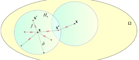
Within the peridynamic framework, the interaction between material points is nonlocal. Therefore, a material point is influenced by the other material points within its neighborhood defined by its horizon. As shown by Oterkus et al. [9], the PD form of Eq. (1) can be derived as

( )

(

)

( )

1

,

_H

, , , ,

,

m

ψ

t

=

_∫

f

ψ ψ

′

′

t dV

_′

+

s

t

x x

x

x x

x

(2)

where f is the response function which governs the

interaction between material points x and x′. It enables the exchange of field variable between material points that are

connected through bonds. In Eq. (2), the parameter

H

x

represents the domain of influence region for the material point at x as shown in Fig. 1. Its extent is defined by the parameter,

δ

referred to as the horizon. The response

function, f is zero for material points outside the horizon;

i.e., x x_{′− >}

_δ

. The pairwise response function can be

defined as

(

, , , ,

)

( ) ( )

',t ,t f

ψ ψ

′ ′ t =m

ψ

′ −

ψ

′ −

x x

x x

x x (3)

where m is the PD material parameter which is dependent on

[image:2.612.329.551.321.418.2]

the material properties and the horizon. This parameter can be determined by equating the PD form of the diffusion equation to the classical diffusion equation as the horizon size approaches to zero. The explicit form of this parameter is given in the subsequent sections for three different physical fields, i.e. temperature, moisture concentration and electrical potential.

Fig. 1. Interaction of material point x with its neighboring

point, x′

A. Thermal diffusion

If the field variable,

ψ

in Eq. (1) represents temperature,

Θ, the parameters in Eq. (1) are defined as

m

₁

=

ρ

c

_v and

2 T

m

=

k

with k_T, c_v and

ρ

representing the thermal conductivity, specific heat and density, respectively, and

T

s q

=

is the volumetric heat generation. Thermal response

function is denoted by f_T

(

Θ Θ′, , , ,x x′ t

)

. The response

function enables the exchange of heat between material points that are connected through thermal bonds. The PD material parameter, m corresponds to the micro-thermal conductivity,

T

2 3 4 2 (1-D) 6 (2-D) 6 (3-D) T T T T T T k A k h k κ δ κ π δ κ πδ = = = (4)

in which h is the thickness of the plate and A is the cross

sectional area. The heat flux, q, which is the rate of flow of

heat energy through a surface, is defined as

T

k

=

− ∇Θ

q

(5)

As derived by Oterkus et al. [10], the corresponding peridynamic heat flux can be expressed as

( ) ( )

1 ( )

', ,

2 H

κ

T t t dV′

′ − ′

=−

∫

⎡_⎣Θ − Θ ⎤_{⎦ ′−}

x x

x x

q x x

x x (6)

B. Moisture diffusion through wetness field

The moisture diffusion equation can be recovered if the

field variable,

ψ

in Eq. (1) is defined as concentration,

C

_M

with

m

₁

=

1

and

m

₂

=

D

_M representing moisture diffusion

coefficient. However, the diffusion equation, Eq. (1) is only valid for a homogenous domain. Therefore, it is not valid for direct solution of concentration in nonhomogeneous domains because the concentration is not continuous along dissimilar interfaces. In order to remedy this situation, Wong et al. [14] introduced a normalized field variable called “wetness” as

sat C w

C

= (7)

They showed the continuity of this new field through the interface of dissimilar materials based on the equalization of chemical potentials. Therefore, the moisture concentration can be determined by solving first for wetness. The diffusion equation, Eq. (1) can be recast in terms of the wetness field as

w

ψ

= . If the source function,

s

( , )

x

t

at material point x has a

non-zero value, the second term on the right hand side of Eq.

(1) requires a modification as

s

( , )/

x

t C

_sat. However, this

equation is only valid under time independent moisture

concentration,

C

_sat condition.

Consequently, the moisture concentration response

function is denoted by f_M

(

w w′, , , ,x x′ t

)

, and it enables

exchange of wetness between material points that are connected through hygro bonds. The PD bond constant, m,

corresponds to the micro-moisture diffusivity,

κ

_M and can be

defined as 2 3 4 2 (1-D) 6 (2-D) 6 (3-D) M M M M M M D A D h D κ δ κ π δ κ πδ = = = (8)

C. Electrical conduction

If the field variable,

ψ

in Eq. (1) represents electrical

potential, Φ, the parameters in Eq. (1) are defined as

m

₁

=

c

_E

and

m

₂

=

k

_E with k_E and c_E representing the electrical

conductivity and the electrical capacitance, respectively. The

electrical response function is denoted by f_E

(

Φ Φ′, , , ,x x′ t

)

,

and it enables exchange of electrical current between material points that are connected through electrical bonds. The PD bond constant, m corresponds to the micro-electrical

conductivity,

κ

E and can be defined as

2 3 4 2 (1-D) 6 (2-D) 6 (3-D) E E E E E E k A k h k κ δ κ π δ κ πδ = = = (9)

Classically, the current density vector, j can be expressed in

E

k

=

− ∇Φ

j

(10)

The corresponding peridynamic current density vector in terms of the response function can be expressed as [10]

(

)

1 ( )

( , ) , , , ,

2 E

H

t =− f Φ Φ′ ′ t ′ − dV_′

′ −

∫

x

x

x x

j x x x

x x (11)

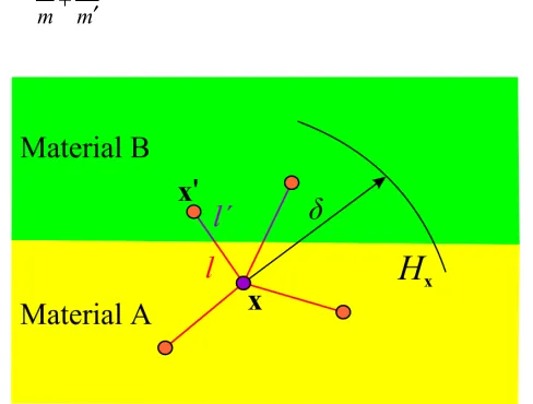
As shown in Fig. 2, material points, x and x′ can be located on opposite sides of the interface with different coefficients m

and m′, respectively. The PD bond between material points

x and x′ is split between these two materials. The segments of this bond are associated with these material points and are denoted by l and l′, respectively. The property of this bond

between material points, x and x′ can be approximated as

l l m

l l m m

′ +

= _′

+ ′

[image:4.612.51.295.350.535.2]

(12)

Figure 2. PD interactions of material points near the interface region.

III. PERIDYNAMICMODELINGOFDIFFUSIONVIA FINITEELEMENTMETHOD

The implementation of PD modeling is explained by considering thermal diffusion analysis because many commercial finite element software readily offers heat transfer analysis capability. Moisture and electrical conduction analysis can be performed by using the same methodology

after successfully calibrating the parameters associated with the thermal diffusion analysis.

As described in the previous section, the bond-based PD heat conduction equation can be written as

'

v T T

c f dV h

ρ

Η

Θ=

_∫

+ (13a)

where ρ is density, cv is specific heat capacity, hT is heat

source and fT is the thermal response function which is

defined as

' T T f =

κ

Θ − Θ

′ −

x x (13b)

in which

κ

_T is thermal micro-conductivity, Θ is temperature

of material points, and ξ = x x′− is the reference length

between material points. The PD equation of heat conduction can also be expressed in discretized form for the material point

located at x_i as

ij i

v i T j T j

c f V h

ρ Θ =

∑

+ (14a)

with

ij

j i

T T

j i f =κ Θ − Θ

−

x x (14b)

where the subscript j represents the parameters associated with the family members of the main material point, x_i.

The classical heat conduction equation is of the form

2

v T T

c k h

ρ

Θ= ∇ Θ+ (15)

where k_T is thermal conductivity. By comparing this

2

ij

T T j

j

k ∇ Θ →

∑

f V (16a)

or

2 j i

T T j

j j i

k ∇ Θ →κ Θ − ΘV

−

∑

_{x x} (16b)

In light of Eq. (16), it is apparent that weak form of Eq. (15) can be recast similar to Eq. (14a) provided that certain parameters of the classical equation are calibrated to obtain the appropriate form of the PD equation.

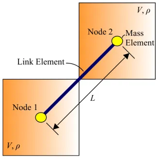
Considering a one-dimensional heat flow between two mass elements, which are connected to each other with a link element as shown in Fig. 3, the weak form of Eq. (15) or its finite element equation can be expressed as

[ ]

M

{ }

Θ +

[ ]

K

{ } { }

Θ = F (17)

in which

[ ]

M is the lumped mass matrix in terms of mass

elements which depend on density ρ, specific heat capacity cv

and volume V of each node. Moreover,

[ ]

K is the stiffness

matrix of the link element,

{ }

F vector represents the heat

[image:5.612.89.253.473.637.2]

source at each node and

{ }

Θ is the nodal temperature vector.

Figure 3. Thermal link and thermal mass elements to represent PD heat conduction

Furthermore, Eq. (17) can be explicitly written as

1 1

1

2 2

2

1 0 1 1

0 1 1 1

T T v T h Ak

c V V

h L

ρ

⎡⎢ ⎥⎤⎨ ⎬⎪ ⎪_{⎪ ⎪}⎧ ⎫Θ_Θ + ⎡⎢₋ − ⎤_{⎥ Θ}⎧ ⎫⎨ ⎬Θ = ⎧ ⎫⎨ ⎬

⎣ ⎦⎩ ⎭ ⎣ ⎦ ⎩ ⎭ ⎩ ⎭ (18)

in which subscripts 1 and 2 represent nodes 1 and 2, respectively. The volumes of mass elements, i.e., V, are equal and L is the length of the link element.

The peridynamic counterpart of Eq. (18) can be written by multiplying both sides of Eq. (14a) with the volume of the material point, Vi, and considering only heat flow between two material points or nodes as shown in Fig. 3 as

i j i

v i i i T j i T

j _{j i}

c V V V V h

ρ Θ = κ Θ − Θ + −

∑

_{x x} (19)

For nodes 1 and 2, Eq. (19) can be rewritten as

1 1

1 1 1 1

1 j

v T j T

j _j

c V V V V h

ρ Θ = κ Θ − Θ +

−

∑

_{x x} (20a)

and

2 2

2 2 2 2

2 j

v T j T

j j

c V V V V h

ρ Θ = κ Θ − Θ +

−

∑

_{x x} (20b)

Since the volumes of the material points are equal, i.e.

1 2 j

V =V =V =V due to uniform discretization, Eq. (20) can

be expressed in matrix form as

1 2 2 1 1 2 2

1 0 1 1

0 1 1 1

T T v T h V

c V V

h

κ

ρ

⎡_{⎢ ⎥}⎤_{⎨ ⎬}⎪ ⎪⎧ ⎫Θ + ⎡_⎢ − ⎤_{⎥ Θ}⎧ ⎫_{⎨ ⎬}Θ = ⎪ ⎪_{⎨ ⎬}⎧ ⎫ −

Θ ⎪ ⎪

⎣ ⎦⎩ ⎭ ξ ⎣ ⎦ ⎩ ⎭ ⎪ ⎪⎩ ⎭ (21)

Comparing stiffness matrices,

[ ]

K of both equations, i.e. Eqs.

(18) and (21), the classical parameters can be related to their PD counterparts as

2

T T

since the length of each link element is equal to the reference

length between material points, i.e. L=ξ. The calibration

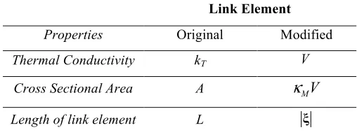
[image:6.612.46.298.209.311.2]

procedure of a link element to represent the PD model is given in Table 1. Moreover, similar calibration procedure can be applied for moisture concentration and electrical conduction fields. The calibration procedures for these fields are given in Tables 2 and 3.

Table 1 Calibration of a link element for thermal analysis

Link Element

Properties Original Modified

Thermal Conductivity kT V

Cross Sectional Area A

κ

_T

V

[image:6.612.45.299.347.445.2]

Length of link element L ξ

Table 2 Calibration of a link element for moisture analysis

Link Element

Properties Original Modified

Thermal Conductivity kT V

Cross Sectional Area A

κ

_M

V

[image:6.612.44.300.501.600.2]

Length of link element L ξ

Table 3 Calibration of a link element for electrical conduction

Link Element

Properties Original Modified

Thermal Conductivity kT V

Cross Sectional Area A

κ

_E

V

Length of link element L ξ

In order to construct the PD model of the domain, link elements can be created between the main material point and its family members within its horizon as shown in Figs. 4a-b. Thus, considering each node as the main material point, and creating link elements between the point itself and its family members lead to a network of link elements (connectivity) as

shown in Fig. 4c. This procedure allows establishment of the global stiffness matrix of the domain. Moreover, mass elements are introduced on top of each node in order to establish the diagonal global mass matrix.

If ANSYS, a commercially available finite element analysis software, is utilized as the computational platform, LINK33 3-D conduction bar element can be used as the thermal link element. For this element, the cross-sectional area of the element, A, should be defined as a real constant.

(a) Family members of the main material point

[image:7.612.81.267.48.189.2]

(c) Network of link elements

Figure 4. PD discretization of a structure with thermal link and thermal mass elements

The material properties of the link elements require correction if its nodes do not have a complete set of family members such as the case for nodes located close to the

surfaces. The determination of surface correction factor,

α

c is

explained by Madenci and Oterkus [11]. Moreover, as demonstrated in Fig. 4(a), the family members (nodes) close to the horizon boundary do not have complete volumes inside the horizon. Hence, it is necessary to determine the “volume”

correction factor,

υ

c for these nodes. Therefore, a more

accurate calibration can be achieved by incorporating these correction factors as

(

c T

)( )

c

A→

α κ υ

V (23)

Note that the link elements should be defined as massless elements by assigning a material with zero density value because the total mass of the structure is represented by using thermal mass elements. For the mass element, MASS71 thermal mass element is suitable. The density,

ρ

and specific

heat capacity, c_v can be defined as material property whereas

the volume of the material point, Vi can be specified as a real

constant for this element type. For moisture diffusion through

wetness analysis, the density,

ρ

and specific heat capacity, c_v

should be specified as unity. Moreover, for the electrical conduction analysis, the density,

ρ

can take a value of unity

whereas specific heat capacity, cv should be specified as the

electrical capacitance, c_E.

IV. NUMERICAL RESULTS

The numerical results concern the verification of this PD implementation by considering four different problems: (1) heat conduction in a finite bar, (2) heat diffusion in a plate under thermal shock, (3) heat diffusion in a plate of dissimilar materials with an insulated interface crack, and (4) moisture absorption in a three-dimensional material. For validation purposes, the PD predictions are compared with traditional finite element predictions or analytical solutions.

A. Heat conduction in a finite bar

The bar has a length of L=1m and a cross sectional area

of _{A=1 10×} −4_m2 _{with material properties,}

4 2 1.1535 10 /

T v

k c m s

α

₌

ρ

_{= ×} − _{with 396}

T

k = W m C. It

has an initial temperature field of _Θ

(

_{x t}, ₌0

)

₌0o_{C, and its}

ends are subjected to a constant temperature of

(

_x 0,_t

)

(

_{x L t},

)

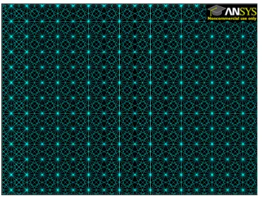
100o_C

Θ = =Θ = = . These boundary conditions are applied to a fictitious region outside of the actual bar region with a length equivalent to the horizon size. As shown in Fig. 5, the PD model has uniform spacing between the

nodes of _{Δ=1 10 m×} −2 _{resulting in 100 nodes, and the}

horizon is specified as

δ

=3.015Δ. Implicit time integration

is utilized with a time step size of Δt=10 s.

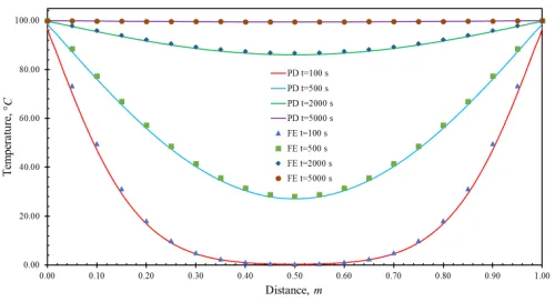
The PD predictions of temperature variation along the bar is shown in Fig. 6 at different times, and they are compared with the traditional FEA predictions. As evident from Fig. 6, both PD and FEA results agree very well with each other.

[image:7.612.313.567.617.673.2]

[image:8.612.321.559.49.201.2]

Figure 6.PD temperature variation along the bar at different times and its comparison with FEA solutions.

The horizon is related to the grid size. Therefore, convergence of the PD predictions to the local solution of diffusion equation is analyzed by considering various values of horizon and grid spacing. Tian and Du [15] developed Asymptotically Compatible (AC) discretization schemes for robust approximations of PD models and their local limit models. AC schemes allow for the preservation of the consistency between nonlocal and local limits of the continuum model at the discrete level, regardless of how the grid spacing between the material points is compared with the horizon.

The horizon is specified as

δ

=m xΔ for decreasing value of uniform spacing between the integration points,

0.0025, 0.005, 0.01, 0.02 and 0.05 m

x

Δ = with a fixed value

of m=3. The number of family members remains the same. Fig. 7 shows the error measure and convergence rate for varying times of t=100, 500, 2000, 5000 s. The PD results converge to the local solution while Δx reduces from 0.05 to 0.0025 m. Similarly, the effect of nonlocality on the convergence rate is studied for a fixed value of Δx=0.0025m

for varying m=1,3,6,12, 24 and 60. The number of family members increases. As shown in Fig. 8, the local solution is obtained as the horizon size reduces to zero and the effect of non-locality increases with the increasing horizon size.

The global error measure is based on

( )

(

( ) ( )

)

2

1 max

1

1

K

e c

m m

e

m

u

u

K

u

ε

=

=

∑

−

where ( )

max

e

[image:8.612.49.299.51.187.2]

u

denotes the maximum of absolute value of exact field variable, the superscripts e and c show the exact and numerical solutions, respectively and K is the total number of points, in which the results are read, in the domain.

Figure 7. Convergence rate for decreasing grid size for a fixed value of m = 3 at varying times.

Figure 8. The effect of nonlocality on the convergence rate for a fixed value of Δx=0.0025 m for increasing m at different

times.

B. Plate under thermal shock

A square plate of isotropic material under thermal shock loading with insulated boundaries at the top and bottom surfaces was considered as shown in Fig. 9. The plate has a length and width of L W= =10 m, and thickness of H=1 m.

Its specific heat capacity, thermal conductivity and mass

density are specified as

c

_v

=

1 J/kgK

,

k

_T

=

1 W/mK

and

3

1 kg/m

ρ

= , respectively. It is subjected to the following initial conditions and boundary conditions:

( , ,

x y t

0) 0 C

Θ

= = °

(24)

and

,x(x 10, ) 0, y t 0

Θ = = > (25a)

,y( ,x y 5) 0, t 0

[image:8.612.315.561.250.389.2]

2 (_x 0, ) 5_{t te}−t, _t 0

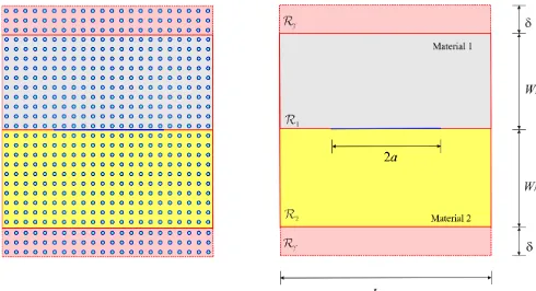
Θ = = > (25c)

As shown in Fig. 9, the spacing between material points in the PD model is Δ=0.1 m and the horizon is specified as

3.015

δ

= Δ. The time step size is kept small even if the problem is solved implicitly in ANSYS in order to capture appropriate wave characteristics. Hence, it is specified as

4 5 10 s

t −

Δ = × .

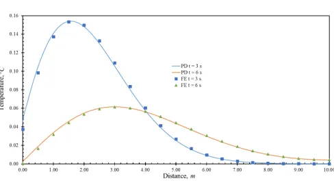
The temperature variations at y=0 are predicted for

3 s

[image:9.612.324.554.48.468.2]

t= and t=6 s. PD results are compared with the FEA predictions as shown in Fig. 10 and they are in close agreement. Furthermore, Fig. 11 demonstrates PD temperature contour plots for the specified times.

Figure 9. Peridynamic model of the plate under thermal shock loading.

Figure 10.Comparison of temperature variations from peridynamics and FEA at y=0.

(a) t=3 s

[image:9.612.45.296.306.437.2]

(b) t=6 s

Figure 11.Thermal shock wave propagation in the plate at different times

C. Dissimilar materials with an insulated crack

As shown in Fig. 12, a square plate made of two different materials with an insulated interface crack is subjected to thermal loading. The plate geometry is specified by a length of L=1 m, width of W=1 m, thickness of H =0.01 m and

crack length of 2a=0.2 m. Its specific heat capacity,

thermal conductivity and mass density are specified as

1 J/kgK

v

c

=

,

k

T

= =

k

1.14 W/cmK

and

ρ

=1kg/cm3,

[image:9.612.52.296.488.620.2]

( , , ,0) 0,

x y z

L

/2

x L

/2,

W

/2

y W

/2

Θ

=

−

≤ ≤

−

≤ ≤

(26)

and

o o

( , /2, ) 100 C, ( ,x W t x W/2, )t 100 C, t 0

Θ = Θ − =− > (27a)

,x( /2, , ) 0, L y t ,x( L/2, , ) 0, y t t 0

Θ = Θ − = > (27b)

The spacing between material points in the PD model is

0.01 m

Δ= and the time step size is specified as Δt=1 s. The problem is solved using 3 different thermal conductivity

values for material 1 and 2 as

k

₁

= =

k

₂

k

;

1

/ 2 and

2

[image:10.612.319.563.51.174.2]

k

=

k

k

=

k

;

k

₁

=

k

/10 and

k

₂

=

k

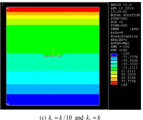
. The peridynamic predictions and their comparison with FEA across the interface are given in Fig. 13. As depicted in this figure, the results have a close agreement with each other. Furthermore, the influence of insulated pre-crack on temperature variations are apparent as shown in Fig. 14 through the contour plots of PD predictions.

[image:10.612.324.556.231.654.2]

Figure 12.Peridynamic model of a square plate with an insulated interface crack.

Figure 13.Temperature variations along x=0, across the

interface of the plate at t=500 s

(a)

k

₁

= =

k

₂

k

[image:10.612.50.295.421.554.2]

[image:11.612.52.297.47.253.2]

(c)

k

₁

=

k

/10 and

k

₂

=

k

Figure 14.PD temperature fields for different types of bimaterial models at t=500 s

D. Moisture absorption of a three dimensional underfill material

This problem demonstrates moisture absorption and weight gain in a three dimensional underfill material. The geometrical parameters are shown in Fig. 15 and they are specified as length, L = 42 mm, width, W = 37.7 mm and thickness, H = 1.2 mm which is much smaller than its length and width. Furthermore, the diffusivity and saturated concentration values of an underfill material are specified as

8 2

1.026 10 m /hr

D_{= ×} − _{and 12.50 kg/m}3

sat

[image:11.612.314.564.141.275.2]

C = , respectively.

Figure 15. Geometrical parameters of the underfill material

The boundary conditions at the outer surfaces are specified as

sat

C C

=

. The material is initially dry, i.e. C x t

(

, = =0

)

0. It

is subjected to moisture absorption for 120 hours. A time step size of 1 hour is specified in the construction of the solution. Eighteen nodes are used in the thickness direction and the horizon size is chosen as

δ

=1.733Δx. Peridynamic result of

the weight change is shown in Fig. 16 and it is compared

against the theoretical result at the fully saturated state. The underfill material reaches its fully saturated weight as

calculated by _{2.3751 10 kg}5

sat sat

W =L W H C× × × = × − which

is in good agreement with the PD prediction.

Figure 16.Comparison of PD and analytical weight gain results

V. CONCLUSION

This study presents the implementation of PD diffusion analysis through a commercial finite element analysis software, ANSYS. It offers several computational benefits including significant reduction of computational time as a result of implicit time integration instead of explicit time integration which is a common approach used in the PD applications. Moreover, very large system of equations can be solved by employing efficient solvers available in ANSYS software.

The accuracy and capability of this implementation are demonstrated by considering four benchmark problems concerning heat transfer and moisture diffusion. Peridynamic predictions compare well with either traditional finite element or analytical solutions. Finally, it is shown that peridynamics can easily deal with the problems including discontinuities in the form of an interface crack between two dissimilar materials.

REFERENCES

[1] Tian, X. and Du, Q., Gunzburger, M. 2016, “Asymptotically compatible schemes for the approximation of fractional Laplacian and related nonlocal diffusion problems on bounded domains,” Advances in Computational

[image:11.612.48.298.511.566.2]

[2] Tian, H. Ju, L.; Du, Q. 2015, “Nonlocal convection–diffusion problems and finite element approximations,” Computer Methods in Applied Mechanics

and Engineering, Vol. 289, Pages 60-78.

[3] Tian, X. and Du, Q. 2014, “Asymptotically compatible schemes and applications to robust discretization of nonlocal models,” SIAM J. Numer. Anal. Vol. 52, pp. 1641-1665.

[4] Silling, S. A., 2000, “Reformulation of elasticity theory for discontinuities and long-range forces,” Journal of the Mechanics and Physics of Solids, Vol. 48 (1), pp. 175-209.

[5] Bobaru, F. and Duangpanya, M., 2010, “The peridynamic formulation for transient heat conduction,” International Journal of Heat and Mass

Transfer, Vol. 53 (19-20), pp. 4047-4059.

[6] Oterkus, S., Madenci, E. and Agwai, A., 2014a, “Peridynamic thermal diffusion,” Journal of Computational Physics, Vol. 265, pp. 71-96. [7] Oterkus, S., Madenci, E. and Agwai, A., 2014b, “Fully coupled

peridynamic thermomechanics,” Journal of the Mechanics and Physics of Solids, Vol. 64, pp. 1-23.

[8] Gerstle, W., Silling, S., Read, D., Tewary, V. and Lehoucq, R., 2008, “Peridynamic simulation of electromigration,” Comput Mater Continua, Vol. 8 (2), pp. 75-92.

[9] Oterkus, S., Madenci, E., Oterkus, E., Hwang Y., Bae, J. and Han, S., 2014, “Hygro-Thermo-Mechanical Analysis and Failure Prediction in Electronic Packages by Using Peridynamics,” 64th Electronic

Components & Technology Conference, Lake Buena Vista, Florida, USA.

[10] Oterkus, S., Fox, J. and Madenci, E., 2013, “Simulation of electro-migration through peridynamics,” IEEE 63rd _{Electronic Components and}

Technology Conference, pp. 1488-1493.

[11] Madenci, E. and Oterkus, E., Peridynamic Theory and Its Applications, Springer (2014)

[12] Silling, S.A. and Askari, A., “A meshfree method based on the peridynamic model of solid mechanics,” Computers & Structures, Vol. 83, No. 17–18, 2005, pp. 1526–1535.

[13] Macek, R. W. and Silling, S. A., 2007, “Peridynamics via finite element analysis,” Finite Elements in Analysis and Design, Vol. 43 (15), pp. 1169-1178.

[14] Wong, E. H., Teo, Y. C. and Lim, T. B., 1998, “Moisture diffusion and vapor pressure modeling of IC packaging,” Proceedings of the 48th

Electronic Components and Technology Conference, pp. 1372-1378.